
21
DESIRABLE AND UNDESIRABLE CONGESTIONS
21.1 INTRODUCTION
This chapter1 discusses the occurrence of congestion within the framework of DEA environmental assessment. As an extension of Chapter 9 on congestion, this chapter now separates the concept of congestion into undesirable and desirable categories in DEA environmental assessment. See Figures 9.1 to 9.4 for a visual description on an occurrence of congestion in a conventional context of DEA. After the separation, this chapter discusses how to measure an occurrence of desirable congestion (DC), or eco‐technology innovation, in comparison with that of undesirable congestion (UC). The concept of DC and UC has a close linkage with, respectively, returns to scale (RTS) and damages to scale (DTS) in Chapter 20. The comparison between Chapters 20 and 21 provides us with extended implications on RTS and DTS from an occurrence of the two types of congestion. The two chapters will be further conceptually and methodologically extendable into other scale measures in Chapter 23.
A concern of this chapter is that the identification of UC is indeed important for avoiding a cost increase and a shortage of transmission capacity in the case of the electric power industry, for example. However, the identification of DC is more important than that of UC in terms of our sustainable growth in which eco‐technology innovation can effectively reduce the amount of various types of pollution. Therefore, it is necessary for this chapter to discuss the occurrence of UC under natural disposability and that of DC under managerial disposability.
As an illustrative application, this chapter applies the proposed approach to evaluate the performance of coal‐fired power plants in PJM, which is a well‐known regional transmission organization, in the United States. See Chapter 14 on a detailed description of PJM. This chapter finds that the occurrence of UC, due to a capacity limit of generation and transmission, is found in most of power plants. In contrast, the occurrence of DC, due to eco‐technology innovation, is found in a limited number of power plants. Thus, the identification of DC assists us in determining how to facilitate eco‐technology innovation for the growth of corporate sustainability. Such determination can be identified by the DEA approach proposed in this chapter.
The remainder of this chapter is organized as follows: Section 21.2 summarizes differences between UC and DC. Section 21.3 formulates radial models under natural disposability. Section 21.4 reformulates them under managerial disposability. Section 21.5 applies the proposed approach to examine the type of UC and DC of United States coal‐fired power plants. Section 21.6 summarizes this chapter.
21.2 UC AND DC
Figure 21.1, originated from Figure 15.7, depicts conceptual differences between UC and DC. The occurrence of UC is usually due to a capacity limit on part or whole production facility, as depicted at the top and the bottom left‐hand side of the figure, while that of DC may be due to eco‐technology innovation and/or managerial challenge for pollution mitigation, as depicted at the bottom right‐hand side of the figure.
FIGURE 21.1 Undesirable congestion (UC) and desirable congestion (DC) (a) Each occurrence of congestion is classified into three categories: strong, weak and no. (b) The top of the figure indicates the possible occurrence of UC within a conventional DEA framework on x and g. This type of congestion has been long discussed in the DEA community. See Chapter 9. (c) The bottom left‐hand side indicates the possible occurrence of UC in which an enhanced component(s) of an input vector increases some component(s) of the undesirable output vector, but decreases some component(s) of the desirable output vector. The equality constraints without slacks should be assigned to undesirable outputs (B) in the proposed formulations. (d) The bottom right‐hand side indicates the possible occurrence of DC, or eco‐technology innovation for pollution mitigation. In DEA environmental assessment, this type of occurrence indicates that an enhanced component(s) of an input vector increases some component(s) of a desirable output vector, but decreases some component(s) of an undesirable output vector. This study thinks that eco‐technology innovation can solve various pollution issues, so that the occurrence of DC is important in DEA environmental assessment. For identifying the possible occurrence of DC, equality constraints without slacks are assigned to desirable outputs (G) in the proposed formulations. (e) The convex function at the bottom right‐hand side depends upon the assumption that undesirable outputs (B) are “byproducts” of desirable outputs (G). It should be a concave function without such an assumption. The assumption is acceptable and realistic as long as DC occurs on B. See Chapter 15 on the assumption.
The top of Figure 21.1 exhibits an efficiency frontier and the classification of UC in a desirable output (g) on the vertical axis and an input (x) on the horizontal axis. The classification has been used in a conventional framework of DEA, as discussed in Chapter 9. In a similar manner, the bottom left‐hand side exhibits the classification of UC on an undesirable output (b) on the horizontal axis and a desirable output (g) on the vertical axis. The opposite case is found in the bottom right‐hand side which classifies the type of DC. The two cases at the bottom are used in the computational framework of DEA environmental assessment, while an occurrence of UC in conventional DEA is depicted at the top of Figure 21.1. For our visual convenience, the three cases of Figure 21.1 consider a single component of three production factors. It is easily extendable to multiple components of these factors in the formulations proposed in this chapter. Note that each piece‐wise linear contour line indicates the relationship between two production factors, depending upon a possible occurrence of UC or DC and these different combinations of production factors.
The rationale concerning why this chapter uses Figure 21.1 is that the concept of congestion, in particular DC, is very important in discussing DEA environmental assessment. However, as summarized in Chapter 28, most previous studies have paid attention to only UC as depicted in the bottom left of the figure as a straightforward extension of the top of the figure. It is true that an occurrence of UC is important in discussing the performance assessment of energy sectors. However, such a research direction toward the UC identification may not be important in discussing environmental assessment.
Before our analytical discussion on UC and DC, this chapter provides Figure 21.1 that visually provides us with an intuitive rationale concerning why an occurrence of congestion is important for environmental assessment. The concept of congestion has been long used by many previous DEA studies. See Chapter 28 that summarizes previous research efforts which have used the concept of “weak disposability” to identify a possible occurrence of UC in DEA. As mentioned in Chapter 9, the identification of a possible occurrence of UC is indeed important in examining a capacity limit on a production facility in energy sectors. However, this chapter directs toward examining the possible occurrence of DC in environmental assessment because we are interested in pollution prevention and reduction. Thus, DC is more important than UC in terms of reducing the amount of industrial pollution by utilizing eco‐technology. The best research strategy is that we examine an occurrence of both UC and DC, as discussed in this chapter.
To describe the classification on the type of UC and DC, let us start the left‐hand side of the bottom of Figure 21.1 in which a supporting line visually specifies the shape of a curve and a possible occurrence of UC. In the figure, a negative slope indicates the occurrence of UC, so being considered “strong UC”. The occurrence implies a case in which a DMU increases an amount of an input (x). The increased input usually enlarges both desirable (g) and undesirable (b) outputs. However, such an input change increases the undesirable output (b) but decreases the desirable output vector (g), as visually specified by the negative slope of the supporting line. It is clear that such an occurrence is “undesirable” to us. In contrast, a positive slope implies the opposite case (i.e., no congestion), so being referred to as “no UC”.
In addition to the two cases, it is necessary for us to consider the third situation in which the slope of the supporting line is zero; this chapter considers it as “weak UC,” being between strong UC and no UC.
The description of UC is applicable to the occurrence of DC. A possible occurrence of DC, or eco‐technology innovation on undesirable outputs, is depicted in the bottom right‐hand side of Figure 21.1. In this chapter, the occurrence of DC is more important than that of UC, as mentioned previously, because the former case indicates green technology innovation (e.g., clean coal technology). It is believed that only the eco‐technology innovation may have a potential to solve various environmental problems (e.g., air and/or water pollution), along with managerial challenges (e.g., a fuel mix strategy from coal to renewable energy). As depicted in the bottom right‐hand side of Figure 21.1, the negative slope of the supporting line indicates such an occurrence of DC. More specifically speaking, the occurrence implies that an enlarged input (x) increases the desirable output (g) and decreases the undesirable output (b). A possible occurrence of DC is classified into the three categories: no, weak or strong.
Figure 21.2 visually reorganizes the bottom left‐hand side of Figure 21.1 by paying attention to the relationship between a supporting line and the three types of UC: no, weak and strong. The piece‐wise linear contour line indicates the efficiency frontier between the two production factors (g and b). The figure depicts a possible occurrence of UC that is listed at the right‐hand side of the figure, so indicating an occurrence of “unsustainability”. Under such an occurrence, an increase in some component(s) of an input vector increases some components of the undesirable output vector (B) and decreases those of the desirable output vector (G) without worsening the other components. This type of congestion has been long discussed and investigated in a conventional use of DEA. For example, the strong UC indicates an occurrence of a line limit on transmission capacity between a generator and consumers. In contrast, the left‐hand side of Figure 21.2 depicts “economic sustainability” where a firm can attain economic success, but lacking environmental protection. See Chapter 9, which does not consider the existence of an undesirable output. So, exactly speaking, the previous DEA studies did not consider an occurrence of UC.
FIGURE 21.2 Undesirable congestion (UC) and unsustainability. (b) See Figure 9.5 in which x and g indicate the horizontal and vertical coordinates, respectively. Many previous studies extend Figure 9.5 to Figure 21.2 in discussing the occurrence of UC. The identification of UC is important in energy economics because it indicates a capacity limit.
(a) Source: Sueyoshi and Goto (2016)
Shifting our description from UC to DC, Figure 21.3 depicts the occurrence of DC between a single desirable output (g) on the horizontal axis and a single undesirable output (b) on the vertical axis. The figure depicts a possible occurrence of DC. Under such an occurrence of DC, as depicted in the right‐hand side, an increase in some component(s) of an input vector increases some components of the desirable output vector (G) and decreases those of the undesirable output vector (B) without worsening the other components. This type of congestion occurs with eco‐technology innovation on undesirable outputs (B). In contrast, the left‐hand side of the figure indicates an occurrence of “economic sustainability,” where a firm can attain economic success, but lacking an environmental protection capability.
FIGURE 21.3 Desirable congestion (DC) and sustainability.
(a) Source: Sueyoshi and Goto (2016)
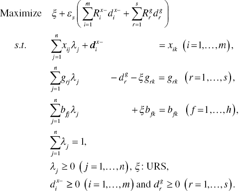
Returning to Equation (15.1) in Chapter 15, a unified (operational and environmental) production and pollution possibility set (P) to express a possible occurrence of UC under natural disposability is axiomatically expressed by

Here, the superscript N, stands for natural disposability with a possible occurrence of UC. Equation (21.1) incorporates ![]() so that corresponding dual variables becomes unrestricted in their signs. Since each dual variable indicates a slope of a supporting hyperplane in the case of multiple components, Equation (21.1) can identify a possible occurrence of UC under natural disposability, as depicted in Figure 21.2. The subscript (v) indicates the status of variable RTS under natural disposabiity and/or variable DTS under managerial disposability. See Chapter 20.
so that corresponding dual variables becomes unrestricted in their signs. Since each dual variable indicates a slope of a supporting hyperplane in the case of multiple components, Equation (21.1) can identify a possible occurrence of UC under natural disposability, as depicted in Figure 21.2. The subscript (v) indicates the status of variable RTS under natural disposabiity and/or variable DTS under managerial disposability. See Chapter 20.
Meanwhile, the set (P) with a possible occurrence of DC, as depicted in Figure 21.3, is formulated under managerial disposability as follows:

where the superscript M, stands for managerial disposability with a possible occurrence of DC. In the above case, we need to incorporate ![]() into Equation (21.2) to identify a possible occurrence of DC.
into Equation (21.2) to identify a possible occurrence of DC.
At the end of this section, this chapter adds two concerns on UC and DC. The first concern is that it is impossible for us to assume constant RTS and constant DTS in the identification of UC and DC because the assumption sets a supporting hyperplane as a straight line, not a curve, passing from the origin. The slopes of the supporting hyperplane are non‐negative under constant RTS and DTS. The situation is inconsistent with the identification of UC and DC. The production and pollution possibility set for UC and DC should be structured by variable RTS and DTS as specified in Equations (21.1) and (21.2). The second concern is that the equality condition (e.g., ![]() ) in the two equations implies no slack in the formulations proposed in this chapter. Thus, the existence of slacks in equality constraints in the proposed (augmented) formulations implies that constraints are functionally inequality for DEA environmental assessment.
) in the two equations implies no slack in the formulations proposed in this chapter. Thus, the existence of slacks in equality constraints in the proposed (augmented) formulations implies that constraints are functionally inequality for DEA environmental assessment.
21.3 UNIFIED EFFICIENCY AND UC UNDER NATURAL DISPOSABILITY
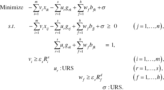
As depicted in Figure 21.2, this chapter can identify a possible occurrence of UC under natural disposability. To examine such an occurrence in the radial measurement, we reorganize Model (17.5) by putting equality constraints (so, no slack variable) on undesirable outputs (B). For such a purpose, this chapter uses a radial model to measure the unified efficiency on the k‐th DMU that reorganizes the original formulation, or Equation (17.5). Following Sueyoshi and Goto (2016), the restructured model becomes
An important feature of Model (21.3) is that it does not have slack variables related to undesirable outputs (B), being different from Model (17.5), so that they are considered as equality constraints. The other constraints regarding inputs and desirable outputs are considered as inequality because they have slack variables in Model (21.3).
Model (21.3) has the following dual formulation:
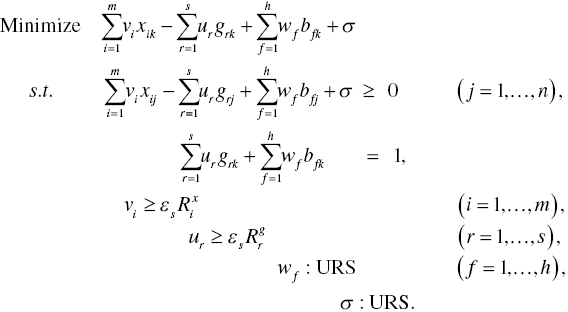
In Model (21.4), all the dual variables related to undesirable outputs (wf: URS for f = 1,…, h) are unrestricted in their signs because the constraints on B are formulated by the equality in Model (21.3).
A unified efficiency, or ![]() , of the k‐th DMU under natural disposability is measured with a possible occurrence of UC. The degree is determined by
, of the k‐th DMU under natural disposability is measured with a possible occurrence of UC. The degree is determined by
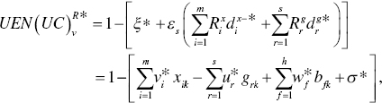
where all variables are determined on the optimality of Models (21.3) and (21.4). The superscript R and the subscript v are related to the radial measurement with variable RTS and DTS. The UC implies a possible occurrence of undesirable congestion. The equation within parentheses, obtained from the optimality of Models (21.3) and (21.4), indicates the level of unified inefficiency under natural disposability. The unified efficiency is obtained by subtracting the level of unified inefficiency from unity as specified in Equation (21.5).
To discuss a mathematical rationale on why Models (21.3) and (21.4) can identify a possible occurrence of UC, this chapter needs to discuss the following proposition:
The proposition implies that the supporting hyperplane measured on the optimality of Model (21.4) is expressed by ![]() on an efficiency frontier in the case of a single component of the three production factors. The hyperplane is also specified by
on an efficiency frontier in the case of a single component of the three production factors. The hyperplane is also specified by ![]() . Since both u * and v * are positive, the slope of the supporting hyperplane is determined by w * and σ *, both are unrestricted in their signs, on the optimality of Model (21.4).
. Since both u * and v * are positive, the slope of the supporting hyperplane is determined by w * and σ *, both are unrestricted in their signs, on the optimality of Model (21.4).
After solving Model (21.4), we can identify the occurrence of UC by the following rule under the assumption on a unique optimal solution:
- If
 for some (at least one) f, then “weak UC” occurs on the k‐th DMU,
 - If
 for some (at least one) f, then “strong UC” occurs on the k‐th DMU and
 - If
 for all f, then “no UC” occurs on the k‐th DMU.
It is important to note three concerns on the classification on UC. First, this chapter assumes a unique optimal solution for our computational tractability. See Chapter 7 on the occurrence of multiple solutions. If multiple solutions occur on the k‐th DMU, it is necessary for us to measure the upper and lower bounds of σ * to prepare the decision on an occurrence of UC. See Chapters 8 and 20 for detailed descriptions on the selection on upper and lower bounds for σ * (i.e., the intercept of the supporting hyperplane). This chapter clearly understands the drawback of our assumption on the unique solution. Second, if ![]() for some f and
for some f and ![]() for the other f ′, then both strong and weak UCs coexist on the k‐th DMU. In this case, we consider the case as an occurrence of the strong UC on the k‐th DMU. Finally, as discussed in Chapter 9, in particular Section 9.5.1, it is necessary for us to project an inefficient DMU onto an efficiency frontier in identifying the type of UC. This chapter does not consider the projection, except noting Models (9.13) and (9.14), to enhance our computational tractability.
for the other f ′, then both strong and weak UCs coexist on the k‐th DMU. In this case, we consider the case as an occurrence of the strong UC on the k‐th DMU. Finally, as discussed in Chapter 9, in particular Section 9.5.1, it is necessary for us to project an inefficient DMU onto an efficiency frontier in identifying the type of UC. This chapter does not consider the projection, except noting Models (9.13) and (9.14), to enhance our computational tractability.
21.4 UNIFIED EFFICIENCY AND DC UNDER MANAGERIAL DISPOSABILITY
To attain a high level of managerial disposability, a DMU needs to increase some components of the input vector in order to increase some components of the desirable output vector and simultaneously decrease those of the undesirable output vector.
As depicted in Figure 21.3, this chapter can identify a possible occurrence of DC under managerial disposability. To examine the occurrence, this chapter reorganizes Model (17.10) by eliminating slack variables on desirable outputs (G) as follows:
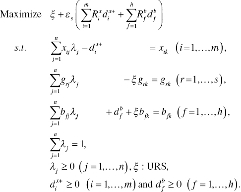
Model (21.18) drops slack variables related to desirable outputs (G) so that they are considered as equality constraints. The other groups of constraints on inputs and undesirable outputs maintain slacks so that they can be considered as inequality constraints. The description on inputs is also applicable to undesirable outputs.
Model (21.18) has the following dual formulation:
An important feature of Model (21.19) is that the dual variables (ur: URS for r = 1,…, s) are unrestricted in their signs because Model (21.18) eliminates slacks related to desirable outputs.
A unified efficiency score, or ![]() , of the k‐th DMU under managerial disposability becomes
, of the k‐th DMU under managerial disposability becomes
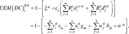
where all variables are determined on the optimality of Models (21.18) and (21.19). The equation within the parenthesis, obtained from the optimality of Models (21.18) and (21.19), indicates the level of unified inefficiency under managerial disposability. The unified efficiency, along with a possible occurrence of DC, is obtained by subtracting the level of inefficiency from unity.
To discuss a mathematical rationale for why Models (21.18) and (21.19) can identify a possible occurrence of DC, this chapter needs to discuss the following proposition:
The supporting hyperplane is expressed by ![]() on an efficiency frontier in the case when three production factors have a single component. The supporting hyperplane in Figure 21.3 is expressed by
on an efficiency frontier in the case when three production factors have a single component. The supporting hyperplane in Figure 21.3 is expressed by ![]() . Since both w* and v* are positive, the slope of the supporting hyperplane is determined by u* and σ*, both of which are unrestricted in their signs.
. Since both w* and v* are positive, the slope of the supporting hyperplane is determined by u* and σ*, both of which are unrestricted in their signs.
After solving Model (21.19), this chapter can identify a possible occurrence of DC, or eco‐technology innovation, by the following rule along with the assumption on a unique optimal solution:
- If
 for some (at least one) r, then “weak DC” occurs on the k‐th DMU,
 - If
 for some (at least one) r, then “strong DC” occurs on the k‐th DMU and
 - If
 for all r, then “no DC” occurs on the k‐th DMU.
Note that if ![]() for some r and
for some r and ![]() for the other r′, then the weak and strong DCs coexist on the k‐th DMU. This chapter considers it as the strong DC, so indicating technology innovation on undesirable outputs. Here, it is important to add that
for the other r′, then the weak and strong DCs coexist on the k‐th DMU. This chapter considers it as the strong DC, so indicating technology innovation on undesirable outputs. Here, it is important to add that ![]() for all r is the best case because an increase in any desirable output always decreases an amount of undesirable outputs. Meanwhile, if
for all r is the best case because an increase in any desirable output always decreases an amount of undesirable outputs. Meanwhile, if ![]() is identified for some r, then it indicates that there is a chance to reduce an amount of undesirable output(s). Therefore, we consider the second case as an occurrence of DC. The three concerns (e.g., multiple solutions and slack adjustment) on UC are also applicable to DC.
is identified for some r, then it indicates that there is a chance to reduce an amount of undesirable output(s). Therefore, we consider the second case as an occurrence of DC. The three concerns (e.g., multiple solutions and slack adjustment) on UC are also applicable to DC.
21.5 COAL‐FIRED POWER PLANTS IN UNITED STATES
21.5.1 Data
Returning to Chapter 18, this chapter uses a data set on 68 PJM’s coal‐fired power plants in 2010. The data source is the Environmental Protection Agency (EPA) database: eGRID year 2010, http://www.epa.gov/cleanenergy/energy‐resources/egrid/index.html. The data set consists of 68 coal‐fired power plants operating in the PJM Interconnection. This chapter excludes plants used for combined heat and power and those under mixed combustion with biomass fuel.
Data Accessibility:
The original data set used in this chapter can be found in the supplementary section of Sueyoshi and Goto (2016).
The generation of each power plant is characterized by a single desirable output, two inputs and three undesirable outputs. The desirable output is measured by the amount of annual net generation (MWh: Megawatt hours). The two inputs are measured by (a) the nameplate capacity (MW: Megawatt) and (b) the amount of annual heat input (MMBtu). The undesirable outputs are measured by three items: (a) the annual amount of NOx emissions (tons), (b) the annual amount of SO2 emissions (tons) and (c) the annual amount of CO2 emissions (tons) at each power plant. The first two belong to acid rain gases, but not GHG. The last one belongs to GHG. In this chapter, each observed data is divided by the factor average to avoid the case where a large data dominates the other small data in DEA computation. Thus, the data set used in the proposed DEA formulations is structured by index numbers so that they are unit‐less.
The type of primary fuel of power plants is classified into two categories. One of the two categories is the bituminous (BIT) coal that is relatively soft coal that contains a tarlike substance, called “bitumen”. The other category is the sub‐bituminous (SUB) coal that is a type of coal whose properties range from those of lignite to those of bituminous coal and are used primarily as fuel for steam‐electric power generation. See Chapter 18 for a a description of coal categories.
21.5.2 Occurrence of Congestion
Table 21.1 summarizes UEN (unified efficiency under natural disposability), dual variables and the occurrence of UC on coal‐fired power plants. For example, the first power plant exhibits a degree of UEN of 0.9625. The power plant exhibits strong UC.
TABLE 21.1 Unified efficiency measures, dual variables and type of undesirable congestion (UC)
(a) Source: Sueyoshi and Goto (2016).
| UEN | |||||
| Bituminous | |||||
| Plant No. | Efficiency Score | NOx | SO2 | CO2 | UC |
| 1 | 0.9625 | −0.0629 | 0.0182 | 1.3073 | Strong |
| 2 | 0.9539 | 0.0458 | −0.0151 | 0.7104 | Strong |
| 3 | 1.0000 | 1.4439 | −0.5288 | 11.6587 | Strong |
| 4 | 1.0000 | 0.0472 | −0.0168 | 0.4172 | Strong |
| 5 | 1.0000 | −0.0026 | 0.0785 | 0.5281 | Strong |
| 6 | 1.0000 | −0.0144 | 0.3202 | 0.4347 | Strong |
| 7 | 1.0000 | 1.8488 | 0.1051 | −0.1169 | Strong |
| 8 | 1.0000 | 0.0666 | −0.0220 | 1.0335 | Strong |
| 9 | 1.0000 | 0.0329 | −0.0083 | 0.2796 | Strong |
| 10 | 0.9303 | −0.0215 | 0.0063 | 0.4481 | Strong |
| 11 | 1.0000 | −2.5143 | 0.5506 | 32.5014 | Strong |
| 12 | 0.8467 | −0.1267 | 0.0708 | 2.9385 | Strong |
| 13 | 0.9752 | −0.0232 | −0.0037 | 0.4755 | Strong |
| 14 | 0.8860 | 0.1535 | −0.0508 | 2.3827 | Strong |
| 15 | 0.9562 | −0.0065 | 0.0001 | 0.2228 | Strong |
| 16 | 1.0000 | −0.0044 | 0.0001 | 0.1499 | Strong |
| 17 | 1.0000 | 0.0076 | 0.2086 | 0.1000 | No |
| 18 | 0.9385 | −0.0045 | 0.0676 | 0.6044 | Strong |
| 19 | 0.9693 | 0.0280 | −0.0098 | 0.3119 | Strong |
| 20 | 1.0000 | 0.0370 | −0.0132 | 0.4173 | Strong |
| 21 | 1.0000 | −0.7091 | 0.1101 | 7.9718 | Strong |
| 22 | 1.0000 | −1.0981 | 0.0226 | 10.4581 | Strong |
| 23 | 1.0000 | −4.3331 | 0.0892 | 41.2671 | Strong |
| 24 | 0.9583 | 3.0147 | −1.1221 | 35.0650 | Strong |
| 25 | 1.0000 | 2.4175 | −0.8998 | 28.1193 | Strong |
| 26 | 1.0000 | 0.0243 | −0.0091 | 0.2830 | Strong |
| 27 | 1.0000 | −0.3632 | −0.0502 | 1.5046 | Strong |
| 28 | 0.9254 | −0.0388 | 0.0112 | 1.5896 | Strong |
| 29 | 1.0000 | −0.0123 | 0.0038 | 0.2556 | Strong |
| 30 | 1.0000 | −0.1063 | −0.0279 | 1.8139 | Strong |
| 31 | 1.0000 | −0.0110 | −0.0018 | 0.1531 | Strong |
| 32 | 0.9454 | −0.0253 | 0.3412 | 2.7654 | Strong |
| 33 | 1.0000 | −0.0149 | 0.2605 | 0.2951 | Strong |
| 34 | 1.0000 | −0.0131 | −0.0075 | 0.2666 | Strong |
| 35 | 1.0000 | 0.0244 | −0.0066 | 0.2043 | Strong |
| 36 | 0.9168 | −0.3172 | 0.0674 | 4.1103 | Strong |
| 37 | 0.9799 | 0.1071 | −0.0355 | 1.6629 | Strong |
| 38 | 1.0000 | −0.0149 | −0.0024 | 0.3054 | Strong |
| 39 | 1.0000 | −0.0063 | −0.0034 | 0.3174 | Strong |
| 40 | 1.0000 | −0.1658 | −0.0411 | 1.3974 | Strong |
| 41 | 0.8300 | 0.1169 | −0.0435 | 1.3592 | Strong |
| 42 | 0.9279 | 0.1333 | −0.0821 | 3.6161 | Strong |
| 43 | 0.9792 | −0.2411 | 0.0419 | 3.2156 | Strong |
| 44 | 0.9169 | −0.0808 | 0.0451 | 1.8723 | Strong |
| 45 | 1.0000 | −0.0233 | 0.4408 | 0.3708 | Strong |
| 46 | 0.8828 | −0.3819 | 0.0812 | 4.9489 | Strong |
| 47 | 0.9674 | −0.0174 | 0.4143 | 0.3689 | Strong |
| 48 | 1.0000 | −0.0021 | 0.0279 | 0.2259 | Strong |
| 49 | 0.9778 | −0.0001 | 0.0271 | 0.3324 | Strong |
| 50 | 1.0000 | −0.0296 | 15.6218 | 191.4309 | Strong |
| 51 | 1.0000 | 0.1081 | 0.0020 | 0.1401 | No |
| 52 | 1.0000 | −0.1915 | 0.0366 | 2.0241 | Strong |
| 53 | 1.0000 | −0.2501 | 0.0478 | 2.6438 | Strong |
| 54 | 1.0000 | 0.0011 | 0.0230 | 0.2771 | No |
| 55 | 1.0000 | 0.0015 | 0.0292 | 0.3516 | No |
| 56 | 1.0000 | 0.0109 | 0.4390 | 0.0978 | No |
| 57 | 0.9616 | −0.0583 | 0.0169 | 1.2134 | Strong |
| Avg. | 0.9752 | −0.0283 | 0.2917 | 7.2123 | |
| Max. | 1.0000 | 3.0147 | 15.6218 | 191.4309 | |
| Min. | 0.8300 | −4.3331 | −1.1221 | −0.1169 | |
| S.D. | 0.0407 | 0.9248 | 2.0823 | 26.3537 | |
| Sub‐bituminous | |||||
| 58 | 0.9104 | 0.1258 | −0.0275 | 1.0466 | Strong |
| 59 | 0.9030 | 0.1950 | −0.0426 | 1.6225 | Strong |
| 60 | 0.8928 | −0.1681 | 0.0422 | 2.2976 | Strong |
| 61 | 1.0000 | −0.1970 | −0.0264 | 0.8359 | Strong |
| 62 | 0.8980 | −0.0145 | −0.0035 | 0.3055 | Strong |
| 63 | 0.9075 | 0.0789 | −0.0211 | 0.6529 | Strong |
| 64 | 0.8943 | −0.0205 | 0.0115 | 0.4754 | Strong |
| 65 | 1.0000 | −0.0089 | −0.0049 | 0.1610 | Strong |
| 66 | 1.0000 | −0.0745 | 0.0162 | 0.9783 | Strong |
| 67 | 0.9531 | −0.1897 | 0.0460 | 3.8360 | Strong |
| 68 | 0.9131 | −2.6907 | 0.5006 | 24.1199 | Strong |
| Avg. | 0.9338 | −0.2695 | 0.0446 | 3.3029 | |
| Max. | 1.0000 | 0.1950 | 0.5006 | 24.1199 | |
| Min. | 0.8928 | −2.6907 | −0.0426 | 0.1610 | |
| S.D. | 0.0455 | 0.8130 | 0.1539 | 6.9851 | |
The UEN of the power plants becomes 0.9752 for bituminous and 0.9338 for sub‐bituminous on total average, respectively. The result on UC indicates that the power plant may face an occurrence of a capacity limit on generation and a line limit on transmission. The status on “No” implies that UC does not occur, for example, in the seventeenth power plant. Thus, Table 21.1 indicates that the occurrence of UC due to a capacity constraint of generation and transmission may be found in most coal‐fired power plants with both bituminous and sub‐bituminous coal combustions.
Meanwhile, Table 21.2 summarizes UEM (unified efficiency under managerial disposability), dual variables and the occurrence of DC due to eco‐technology innovation. For example, the first power plant exhibits a degree of UEM of 1.000 and the power plant exhibits no DC, indicating that it has no such eco‐technology innovation. As found in Table 21.2, the status of strong DC implies that a power plant may have a potential on eco‐technology innovation. The table indicates that such an occurrence of DC is found on a limited number of coal‐fired power plants. Thus, it is suggested that a fuel mix for electricity generation should shift from coal to gas combustion because the latter plants produce more electricity and lower amounts of NOx, SO2 and CO2 emissions than the former plants. Of course, this chapter clearly understands that such a fuel shift is not easy and should be considered under the fuel mix strategy of each electric power company and each nation.
TABLE 21.2 Unified efficiency, dual variables and type of desirable congestion (DC)
(a) Source: Sueyoshi and Goto (2016).
| UEM | |||
| Bituminous | |||
| Plant No. | Efficiency Score | Net Generation | DC |
| 1 | 1.0000 | 0.2805 | No |
| 2 | 0.9811 | 0.0625 | No |
| 3 | 0.9991 | −0.3498 | Strong |
| 4 | 0.9782 | 0.0131 | No |
| 5 | 1.0000 | 0.0197 | No |
| 6 | 1.0000 | 0.0188 | No |
| 7 | 1.0000 | 0.0149 | No |
| 8 | 1.0000 | 0.0487 | No |
| 9 | 1.0000 | 0.0847 | No |
| 10 | 1.0000 | 0.0333 | No |
| 11 | 1.0000 | −2.5259 | Strong |
| 12 | 1.0000 | −1.3858 | Strong |
| 13 | 0.9779 | 0.0041 | No |
| 14 | 1.0000 | −1.5174 | Strong |
| 15 | 1.0000 | 0.0566 | No |
| 16 | 1.0000 | 0.0938 | No |
| 17 | 1.0000 | 0.0664 | No |
| 18 | 0.9992 | 0.0049 | No |
| 19 | 0.9995 | 0.0021 | No |
| 20 | 0.9972 | 0.3554 | No |
| 21 | 1.0000 | 0.5236 | No |
| 22 | 1.0000 | −0.8648 | Strong |
| 23 | 0.9989 | −0.8125 | Strong |
| 24 | 0.9759 | −1.1478 | Strong |
| 25 | 1.0000 | −2.4146 | Strong |
| 26 | 1.0000 | 0.0048 | No |
| 27 | 1.0000 | 0.0061 | No |
| 28 | 1.0000 | 0.0135 | No |
| 29 | 1.0000 | 0.0021 | No |
| 30 | 0.9977 | 0.0747 | No |
| 31 | 1.0000 | 0.0019 | No |
| 32 | 1.0000 | 0.0414 | No |
| 33 | 1.0000 | −0.0994 | Strong |
| 34 | 0.9999 | 0.0022 | No |
| 35 | 1.0000 | 0.0019 | No |
| 36 | 0.9979 | −0.2491 | Strong |
| 37 | 1.0000 | 0.0405 | No |
| 38 | 0.9997 | 0.0044 | No |
| 39 | 1.0000 | 0.0049 | No |
| 40 | 0.9976 | 0.0165 | No |
| 41 | 1.0000 | −0.0353 | Strong |
| 42 | 0.9966 | −0.1231 | Strong |
| 43 | 0.9974 | 0.1252 | No |
| 44 | 1.0000 | −0.8406 | Strong |
| 45 | 1.0000 | −0.0063 | Strong |
| 46 | 0.9983 | −0.2394 | Strong |
| 47 | 0.9961 | −0.0756 | Strong |
| 48 | 1.0000 | 0.0026 | No |
| 49 | 0.9996 | 0.0046 | No |
| 50 | 1.0000 | 2.8589 | No |
| 51 | 1.0000 | 0.0037 | No |
| 52 | 1.0000 | 0.4564 | No |
| 53 | 1.0000 | 0.7201 | No |
| 54 | 1.0000 | 0.0826 | No |
| 55 | 1.0000 | 0.1142 | No |
| 56 | 1.0000 | 0.0693 | No |
| 57 | 1.0000 | 0.3846 | No |
| Avg. | 0.9980 | −0.1047 | |
| Max. | 1.0000 | 2.8589 | |
| Min. | 0.9759 | −2.5259 | |
| S.D. | 0.0056 | 0.7212 | |
| Sub−bituminous | |||
| 58 | 0.9632 | 0.0252 | No |
| 59 | 1.0000 | 0.4667 | No |
| 60 | 0.9627 | −0.1085 | Strong |
| 61 | 0.9773 | 0.0017 | No |
| 62 | 0.9627 | −0.0016 | Strong |
| 63 | 0.9681 | 0.0083 | No |
| 64 | 0.9601 | 0.0017 | No |
| 65 | 0.9784 | 0.1136 | No |
| 66 | 0.9770 | 0.0233 | No |
| 67 | 0.9768 | 0.1006 | No |
| 68 | 1.0000 | 0.4334 | No |
| Avg. | 0.9751 | 0.0968 | |
| Max. | 1.0000 | 0.4667 | |
| Min. | 0.9601 | −0.1085 | |
| S.D. | 0.0141 | 0.1840 | |
Finally, the comparison between Tables 21.1 and 21.2 reveals that the number of DC occurrences, due to eco‐technology innovation, is much lower than that of UC occurrences, due to the capacity limit on generation and the line limit on transmission in US coal‐fired power plants. This provides us with an important policy implication on a fuel mix for electricity generation, as mentioned above.
21.6 SUMMARY
This chapter discussed a new use of DEA environmental assessment to measure an occurrence of DC, or eco‐technology innovation for our sustainable growth, regrading US electric power plants in a comparison with an occurrence of UC in these generation plants. The identification of UC is important to avoid cost increases, tariff increases and shortages of electricity in the electric power industry. This type of congestion is often incurred by a capacity limit on generation and transmission that constitutes a serious obstacle to the efficient use of production factors for electricity supply to consumers. Meanwhile, the identification of DC is important in finding a possible occurrence of eco‐technology innovation that can be effectively used to avoid air pollution so that electric power companies can satisfy governmental standards on environmental protection.
This chapter finds that the UC incurred by a capacity limit on generation and transmission, may occur in most coal‐fired power plants, regardless of the type of coal: bituminous or sub‐bituminous. Meanwhile, the occurrence of DC, due to eco‐technology innovation for sustainable growth, may occur on a limited number of coal‐fired power plants. The result on congestion is useful in determining which technology or type of coal‐fired power plant should receive investment to facilitate eco‐technology innovation for the sustainable management of electric power companies.