2.2 3D Scene Representation with Explicit Geometry – Geometry Based Representation

Geometry-based representations have been the fundamental form to represent 3D objects in the world for decades. Since the dawn of computer graphics, real world objects have been represented using geometric 3D surfaces with associated textures mapped onto them and then the surfaces are rasterized to generate the virtual view using graphics hardware. More sophisticated attributes such as appearance properties can be assigned and used to synthesize more realistic views as well. Point-based representations use a set of discrete samples on the surface to represent the geometry. The sophisticated attributes can be recorded with the surface sample. The sampling density can also be adjusted according to need. In addition, volumetric representation is developed as another branch of geometry-based representations. Volumetric techniques extend the concept of a set of 2D pixels representing a set of unit patches in an image to a set of 3D voxels representing a set of unit volumes of the 3D scene.

Fundamentally, the object can be created by three different methods: manual creation through a user interface such as Maya, results from physical simulation, and results from examination such as MRI or CT scan.

Animation describes the transformation of the objects including the rigid transformation and deformation. Geometry-based representations are generally easier to be manipulated than the image-based representation and the depth-image-based representation. Addition-ally, all animation techniques developed in computer graphics are for geometry-based representations and interested readers can refer to the book written by Parent et al. [10] and this section will not give any further discussion on geometry-based animation.

The rendering process is generally time-consuming and, therefore, there are a large number of acceleration methods to synthesize new views from the set of representations. Currently, graphics hardware has been designed to accelerate the rendering of surface-based representations, and state-of-the-art PC graphics cards have the ability to render highly complex scenes with an impressive quality in terms of refresh rate, levels of detail, spatial resolution, pre-production of motion, and accuracy of textures. These developments in the graphics pipeline give us the possibility of rendering objects in different representations from any viewpoint and direction using the same infrastructure. The achievable performance is good for real-time applications for providing the necessary interactivity. All these fit the need of an interactive 3DTV system to allow users to control the view position and direction efficiently and independently without affecting the rendering algorithm.

There are several limitations in geometry-based representations when applying them to a 3DTV system. These limitations are that the cost of content creation is high since the real world object is generally complex and the model is an approximation with a trade-off between complexity and errors; and the rendering cost depends on the geometric complexity and the synthesized views are still not close to the realism we have come to expect. In this section, we provide a comparative description of various techniques and approaches which constitute the state-of-the-art geometry-based representations in computer graphics.

2.2.1 Surface Based Representation

Objects in the world are generally closed, that is, an object is completely enclosed by a surface. Viewers can only see the surface of most objects and cannot see their interior. Therefore, they can be represented by the outside boundary surface and the representation is called the surface-based representation, which is one of the popular forms in computer graphics. The polygonal mesh is one type of surface-based representations and is used as the basic primitive for the graphics hardware pipeline. The advantage of the surface-based representation is its generality, and it can be used to represent almost all objects. However, the limitation is that the surface-based representation is only an approximation to the original model and potentially requires a huge number of primitives to represent a complex object.

NURBS stands for nonuniform rational B-spline surfaces and is another popular form. The representation uses a set of control points and a two-parameter basis function to represent any point on the surface. The stored data, consisting of their coefficients, is compact, and the resolution can be infinite and adjustable according to the need in precision and the affordable computation speed. The main limitations are the requirement of extra computational process to approximate the surface on the receiver side and its requirement of complexity to represent fine surface detail.

Subdivision surfaces represent an object by recursively subdividing each face of an arbitrary polygonal mesh. The subdivision process allows the sender to send the fundamental polygonal mesh across the channel and reconstruct the surface in desired detail according to the computational ability of the receiver side. However, the limitation is similar to NURBS in keeping the surface detail through the subdivision process, and the extra cost for subdivision.

We will give an introductory description of each representation. Then, a short description of the creation and rendering generally to surface-based representations is also given.

2.2.1.1 Polygonal Mesh Representations

Polygonal meshes are the most popular and common representations for 3D objects in computer graphics. The representation is also the fundamental primitive for graphics hardware pipeline techniques. The main advantage is that the representation can represent any object with almost no topological restrictions. The representation can be adjusted according to the requirement of realism and better approximation. However, those high-precision polygon meshes generally contains millions of polygons. This leads to the main disadvantage that storing, transmitting, and rendering objects with millions of polygons is very expensive. This also leads to a large amount of research in mesh simplification and compression and the results give flexible representations for expressing different levels of detail and progressive quality.

A polygonal mesh represents the surface of a real world object in computer graphics through a collection of vertices, edges, and faces. A vertex is a point in the 3D space which stores the information such as location, color, normal, and texture coordinates. An edge is a link between two vertices. A face is a closed set of edges on the same plane such as a triangle which has three edges and a quadrilateral which has four edges. In other words, a face consists of a set of vertices on the same plane to form a closed loop. A polygonal mesh consists of a set of connected faces. The relationship among vertex, edge and face is illustrated in Figure 2.3. Generally, triangles are the fundamental primitives for any renderer. Some renderers may support quadrilaterals or other simple convex polygons. However, commercially available graphics hardware only supports triangles and quadrilaterals. Generally, triangles and quadrilaterals are good for representing the shape of an object. A surface presents a set of triangles that logically have the same properties or work under the same set of actions. For example, triangles which have the same appearance under the same lighting condition are grouped together to use the same shading information to simulate the appearance of objects. Because of its popularity, different representations are proposed for the need of different applications and goals. The representations vary with the methods for storing the polygonal data including vertices, edges, and faces and the following are the most commonly used ones:

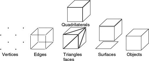
Figure 2.3 The elements for representing an object by polygonal meshes.

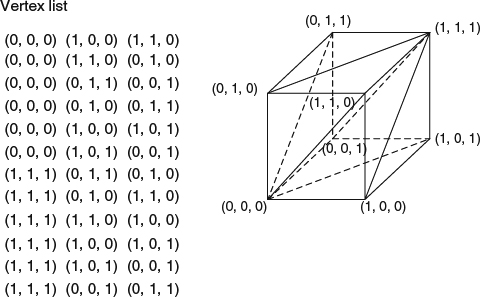
Figure 2.4 A cube is represented with a vertex-vertex mesh.

1. Vertex-vertex meshes

   An object can be viewed as a set of vertices connected to other vertices. Both the edge and face information are implicitly encoded in this representation. This is the simplest representation and is used in DirectX and OpenGL but is not optimized for mesh operations since the face and edge information is implicit because any operation related to faces or edges has to traverse the vertices. Figure 2.4 shows a simple example of a cube represented using a vertex-vertex mesh. This representation uses relatively less storage space and is efficient for shape morphing.

2. Face-vertex meshes

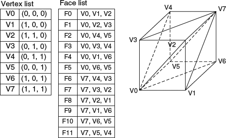
   The representations store a list of vertices and a set of faces consisting of indices to the referred vertices. It is an improvement on vertex-vertex meshes for giving explicit information about the vertices of a face and the faces surrounding a vertex. Therefore, they are more appropriate for certain mesh operations. This is the most common mesh representation in computer graphics and is generally accepted as the input to the modern graphics hardware. For rendering, the face list is usually transmitted to a graphics processing unit (GPU) as a set of indices to vertices, and the vertices are sent as position/color/normal structures (only position is given). This has the benefit that changes in shape, but not topology, can be dynamically updated by simply resending the vertex data without updating the face connectivity. Figure 2.5 shows the face-vertex mesh of a cube. However, the downside is that the edge information is still implicit, that is, a search through all surrounding faces of a given face is still needed, and other dynamic operations such as splitting or merging a face are also difficult.

3. Corner-table meshes

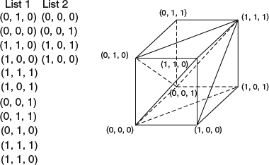
   The representation stores a set of vertices in a predefined table. A special order to traverse the table implicitly defines the polygonal mesh. This is the essential concept for the “triangle fan” used in graphics hardware rendering. Figure 2.6 demonstrates an example of a cube. The representation is more compact than a vertex-vertex mesh and more efficient for retrieving polygons. However, it is harder to represent a surface in a single corner-table mesh and thus multiple corner-table meshes are required.

   

   Figure 2.5 A cube is represented with a face-vertex mesh.

   

   Figure 2.6 A cube is represented with a corner-table mesh.

4. Winged-edge meshes

   This is an extension to face-vertex meshes. Extra edge information includes the index of two edge vertices, the index of the neighboring two faces, and the index of four (clockwise and counterclockwise) edges that touch it. This representation allows traversing the surfaces and edges in constant time but requires more space to store this extra information. Figure 2.7 shows the winged-edge mesh of a cube.

5. Half-edge meshes

   This representation uses a similar concept to a winged-edge mesh but instead of creating an edge table, edge traversal information is recorded in the extra edge traversal information with each vertex. This makes it more space efficient. Figure 2.8 shows the half-edge mesh of the cube.

6. Quad-edge meshes

   This is also a variant of winged-edge meshes. It realizes that a face can be easily recognized by one of its edge and the four edges connected to the face edge. Therefore, the representation only stores vertices and edges with indices to the end vertices and four connected edges. Memory requirements are similar to half-edge meshes. Figure 2.9 shows the quad-edge mesh of a cube.

The representations discussed above have their own pros and cons. A detailed discussion can be found in [14]. Generally, the type of applications, the performance requirement, the size of the data and the operations to be performed affect the choice of representation. In addition, texturing techniques are important to add more lighting details to generate the realistic appearance of objects in computer graphics. Texture techniques can be viewed as wrapping a sheet of 2D detail paper onto different parts of the mesh and generally require some form of texture coordinates to generate proper wrapping. How to apply the texture techniques is also an important consideration when choosing a representation for an application. As a result, there are more variants existing for different applications and still no dominant representation exists. It is still an active research field.

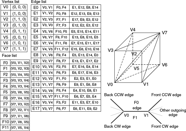
Figure 2.7 A cube is represented with a winged-edge mesh.

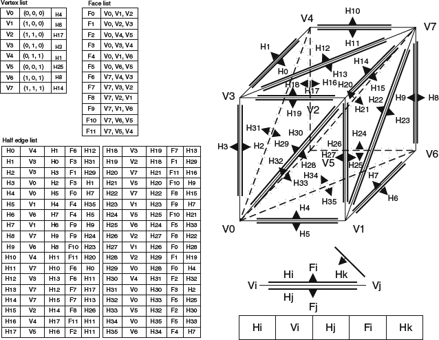
Figure 2.8 A cube represented by half-edge meshes.

2.2.1.2 Polygonal Construction

One category of construction methods for surface-based representations are those generated manually by users. Currently, there is a large range of animation software such as Maya, 3DS Max, and Blender, and computer-aided design (CAD) software such as Autocad available. All of them have the ability to generate polygonal meshes, NURBS surfaces, and subdivision surfaces. 3D animation software gives users the ability to make 3D animations, models, and images and is frequently used for the production of animations, development of games, design of commercial advertisements, and visualization of architecture. They are especially important for movie special effects. CAD tools are used to create the basic geometry for physical simulation and for creating architectural blueprints and product profiles. For example, Abaqus is for mechanical and thermal simulation. All these tools can be used to generate really complex geometry-based objects and also have extra ability to generate different sorts of animations.

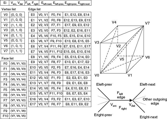
Figure 2.9 A cube represented by a quad-edge mesh.

Another category of methods to construct geometry-based objects is to use a 3D scanner to create a set of samples on the surface of the subject. These samples can be used to create the surface-based representations through a reconstruction procedure. 3D scanners are directly related to depth-image-based content construction. 3D scanners are similar to photographical cameras in terms of a cone-like field of view and collecting information from visible surfaces. In addition to collecting color information, they collect the distance information. In other words the “image” produced by a 3D scanner describes the distance from the scanner to the sample on the visible surface. Generally, a single scan cannot produce a complete model of the world. Multiple scans are needed to obtain all necessary geometrical information for the world. The system requires a common reference and a registration process to combine the result of all scans. The whole process is known as the 3D scanning pipeline [15]. There are different technologies available and they are generally categorized as contact, noncontact active, and noncontact passive 3D scanners [16].

2.2.1.3 Compression and Encoding for Transmission

The number of polygons grows really fast with the advance in the 3D model scanned technology and the requirement for realism. It is hard to transmit and store the entire mesh without compression or simplification. Simplification is useful in order to make storage, transmission, computation, and display more efficient. A compact approximation of a shape can reduce disk and memory requirements and can also speed up network transmission. There are a large number of different simplification or compression methods such as vertex clustering, incremental decimation, resampling, edge collapse, vertex removal, half edge collapse, and so on. Mesh simplification is still an active research field in computer graphics. There is still no algorithm which is better than all others, but the following will only give a short introduction to edge collapse and its reverse operation, vertex splitting because they are popular choices and also the applications for progressivity. We use examples to illustrate the concept of simplification and the ability to progressively deliver a polygonal mesh for coarse-to-fine transmission. Interested readers can refer to [17] for more details.

An example of the edge collapse process is shown in Figure 2.10. First, one edge in the polygonal mesh is picked up according to some global or local error metric which measures the approximation error or the degree of visual fidelity. Then, the end points of the edge are merged into a single vertex and the position of the vertex is updated according to the neighboring vertices. Finally, the faces are updated. Vertex splitting is the reverse of the edge collapse by recording the information necessary to reverse the edge-collapse operation including which vertex is most newly formed and the information of the two merged vertices. Then the collapsed edge can be recovered. In other words, edge collapse is to remove the detail from a polygonal mesh, and vertex split is to recover the details and to increase the accuracy.

A progressive mesh (PM) scheme [18] uses edge collapse and vertex split to achieve the delivery of details in progressive order. In the PM scheme, edge collapse is applied to a fine detailed triangular mesh for creation of a coarser mesh and the resulting coarse mesh can be reconstructed through a sequence of vertex-split refinement operations. Each intermediate mesh along the coarsening sequence corresponds to an LoD approximation. This scheme can automatically support the need of progressive transmission. However, the collapsing criteria are generally based on the global error metric which estimates the degree of approximation to the original model and thus the scheme cannot guarantee smooth transition between consecutive levels. Hoppe et al. [19] proposed a partial fix by incorporating a view-dependent information into the error metric for coarsening the mesh according to visual quality.

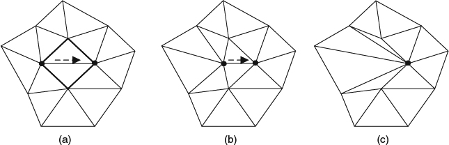
Figure 2.10 The edge collapse process. (a) This is the original mesh. (b) The vertices in the collapse pair move close to each other. (c) Two vertices become one and the connectivity is adjusted to form the new mesh.

There are several variants proposed to relieve the limitation of the original PM scheme. The progressive forest split (PFS) [20, 21] and compressed progressive meshes (CPM) [22, 23] consider several meshes at the same time to form a more space-efficient PM scheme. Progressive time-varying meshes [24] further address the extra dimension of time by considering the deforming meshes at different moments of time. Thus, when considering which edge to collapse, the error metric will take all frames into account and then make the decision. Note that these progressive mesh algorithms are not the most compression-efficient algorithm as extra aided information is needed for progressivity. However, they are important for coarse-to-fine transmission because they allow viewers to get the sense of the viewing scene via a coarse view and the quality can be improved gradually. In addition, during the congestion in the network, the coarse model can still help the transition instead of hanging there without showing anything on the screen.

2.2.1.4 Polygonal Mesh Rendering

Rendering is the process of generating an image of a scene as the result of the interaction between light and the environment. Currently, the popular choice of rendering algorithms is a simple method involving only local information such as the Phong illumination model [25], which is an approximation to the rendering equation [26], or it can be a really complex method involving all objects in the scene such as ray tracing, path tracing and photon mapping.

According to the information involved, the rendering algorithms are generally categorized into:

1. Local illumination

   The local illumination method only considers the relationship between the shading point and light sources and does not take the interaction of light with the environment into account such as object-to-object light interactions (reflections, transmissions etc.). They are only approximations to the direct illumination from light sources on the surface points without considering the occlusion effects. A graphics pipeline generally computes the lighting at each vertex and then uses interpolation techniques such as flat shading, Gouraud shading [27], or Phong shading [25], to fill in the color in each pixel in the scanning line order. Researchers develop advanced techniques such as texture mapping [1, 28], environment mapping [29], and bump mapping [30], to add realism into the rendering results. Generally these techniques are not computationally intensive when compared to global illumination algorithms discussed next and can be implemented in real time on GPUs. Local illumination only involves the lighting computation at each vertex of all primitives in the scene and then the color in each pixel can be computed according to the lighting computations in these vertices. Through careful observation, the lighting computation at each vertex and the color computation at each pixel are independent of those computations for other vertices and pixels. Therefore, the local illumination can be structured as a pipeline to quickly process the computations for vertices and primitives. This pipeline is generally called a graphics pipeline. The process of image generation is called rendering or rasterization with a graphics pipeline which is the most important and popular method of generating images in computer graphics. Generally, primitives used in a graphics pipeline are polygonal meshes and thus surface-based representations will be transformed to a polygonal mesh and then the graphics pipeline is used for rendering.

2. Global illumination

   Global illumination simulates inter-object lighting effects such as reflections and refractions to render more realistic images. However, the computational cost is generally very high.

   • Radiosity [31] can generate a new view by solving the diffuse reflection problem using energy equilibrium equations and is important for rendering interiors in a building and appropriate for architectural walk-throughs. However, the materials allowed to be used in radiosity are limited to diffuse-only materials. This limitation makes it unsuitable for simulating most scenes in the world.
   • Ray tracing algorithms [32, 33] trace the view with rays sent from the camera through each pixel and recursively calculate the intersections of these rays with the scene objects and compute the contribution of light on the intersection points. They can handle specular reflection and refraction. There is a category called photorealistic rendering algorithms. They combine the ray tracing and statistical Monte Carlo methods to estimate the intensity in each pixel. There are several representative algorithms including path tracing [26], bidirectional ray tracing [34, 35], photon mapping [36], and so on. Photon mapping, proposed by Jensen et al. [36], is a two-pass algorithm. The first pass is photon distribution which starts to trace light from light sources to simulate reflections and refractions of light for photons. The second pass is photon collection which is similar to a ray tracing procedure to compute the light contribution at each intersection point according to the photon distribution. The advantage of this algorithm is that it works for arbitrary geometric representations, including parametric and implicit surfaces, and calculates the ray-surface intersections on demand.

The rendering methods are multivarious in the literature. It is not the focus of this book. Interested readers can refer to [37, 38] for more details.

2.2.1.5 Non-uniform Rational B-spline Surface (NURBS) Representations

Polygonal meshes are unorganized representations of surfaces and the approximation error cannot be estimated beforehand. Instead of polygonal meshes, NURBS can describe many shapes without loss of mathematical exactness. NURBS has long been a popular choice in computer aided design (CAD), computer aided manufacturing (CAM), and computer animation because the representations are easily manipulated and with controllable smoothness. NURBS generally defines a patch using a basis function defined by two parameters, u and v. The basis function defines a mapping of a 2D region into the 3D Euclidean space and is usually expressed as the tensor product of some piecewise-polynomial basis functions (B-splines). The patch is specified by a set of 3D control points and two knot vectors to control two parameters, u and v, of the B-spline basis functions. A point on a NURBS patch can be computed as following:

where B is the B-spline basis functions, C is the set of control points for the patch, p and q are degrees (orders) of the surface in u and v directions respectively, and w is the weight for the corresponding control point. Generally, NURBS partitions the entire parameterization domain into subintervals with two known sequences, U = {u₁, u₂, …, u_n} and V = {v₁, v₂, …, v_m}, which are two nondecreasing sets of real numbers. Furthermore, the knot vectors can be nonuniform, that is, the interval between two consecutive knots can be different inside a knot vector. The B-spline basis functions B(u, v) are defined over these knot sequences and can be calculated in a recursive manner. Equation (2.1) associates each knot in a knot sequence with a control point and a basis function. One of the key characteristics of a NURBS patch is that its shape is primarily determined by the positions of its control points. Hence, the influence of each control point is local and this characteristic allows the application to adjust the shape locally by moving only individual control points, without affecting the overall shape of the surface. In addition, the knot vectors can control the shape and smoothness of a NURBS patch. The weight of a control point may make the effect of one control point on a patch different from another. And the weight is a ratio function between two B-spline basis functions and this is why NURBS is rational. Tensor-product uniform B-spline surfaces can be treated as a special case of NURBS with uniform knot vectors and equally weighted control points by setting the denominator to be 1. Interested readers can refer to [39] for mathematical description of NURBS and to [40] for an introduction to the functionality of NURBS in practice.

The main advantages of NURBS is its controllable smoothness within a patch, that is, the continuity can be controlled by the degree of the B-spline basis function. However, mathematical definition of NURBS, which is a tensor product surface, makes it only be able to represent planar, cylindrical, or toroidal topologies. To overcome this topological limitation, a set of NURBS patches can be stitched together to represent an arbitrarily topological surface. Actually, stitching a set of NURBS patches together seamlessly is one of the challenges in the modeling process and generally requires human intervention. There is one solution proposed by Eck et al. [41], but their method is limited to uniform B-splines or to force all patches to have the same knot vector and the same order. This limitation makes it not general to handle all NURBS.

Built-in smoothness is the main advantage of NURBS but this also leads to one of its major drawbacks which is its inefficiency in representing fine surface detail. In order to add a single control point into a patch, an entire column or row of control points must be split to preserve the desired quadrilateral grid structure in the parameter space. A built-in continuity setting may propagate the modification in a control point into the entire surface to generate global effects. The usage of the displacement map [42] is one solution to resolve this problem. The displacement map is a texture storing the fine detail of a model and used to add detail during the rendering process. This scheme is also useful for separating detail from coarser fundamental surface for animation and editing. Another solution is to use a hierarchical NURBS [43]. They work better for editing and refining by providing a valuable coarse manipulation fundamental surface but are hard to generalize for arbitrary complexity and topology.

Infinite resolution is another advantage of NURBS. However, a NURBS patch in practice is tessellated into a polygonal meshes before rendering. Generally, tessellation is achieved by producing a grid of sample points on the parameter space, and then evaluating the position of each sample point accordingly, and linking sample points according to the neighboring information in the parameter space. The density of sampling points can be controlled according to the desired level of detail for the application. However, this built-in LoD does not imply a real incremental LoD representation. A NURBS surface is a compact representation and its LoD hierarchy can be constructed only if the complete representation is available.

2.2.1.6 NURBS Construction

Generally, animation and model software discussed in the previous subsection also provide the tools for creating NURBS. Another commonly used construction method is to fit a NURBS to a polygonal mesh and the method is called surface fitting. The fitting process can be considered as a constrained optimization to construct the surface patchwork and the parameterization. However, they generally either have serious topological limitations [43, 44] or suffer from parameterization distortion, and computational complexity [41]. These limitations can be relieved by human interaction in both patch placement and B-spline patch fitting [42].

2.2.1.7 NURBS Compression and Encoding for Transmission

Since NURBS uses a finite set of control points and a basis function to represent the surface, the representation is compact and is good for transmission. The resolution or precision can be controlled in the receiver side according to the computational ability supported in the receiver end. Therefore progressivity is also supported naturally in this structure.

2.2.1.8 NURBS Rendering

When rendering, generally NURBS surfaces are first transformed to polygonal meshes with proper precision, and then global illumination and local illumination methods for polygonal meshes can be applied directly to generate the images and videos. The downside of this is an extra step for transformation. Additionally, the intersection of a ray with NURBS surfaces can be directly computed and thus ray tracing based methods can be directly used to render the NURBS surfaces.

2.2.1.9 Subdivision Surface Representations

Pixar uses subdivision algorithms in their main production and this has given the technique renewed attention in the past decade as a possible alternative to NURBS and polygonal meshes. The subdivision representation provides an infrastructure to represent a compromise of arbitrary topology and any fine detail with a more controllable smoothness. The basic idea of subdivision is to construct a surface from an arbitrary initial polygonal mesh by recursively subdividing each face in the mesh. When the process is done appropriately, the limited surface to this sequence of successive subdivision will be a smooth surface. For example, Stam [45] proved that the limited surface of the well-known Catmull Clark subdivision scheme can be represented by a bicubic B-spline surface. In the literature, subdivision schemes can be categorized into the following three criteria:

1. the pattern of the refinement rule including vertex insertion [46, 47] and corner cutting [48].
2. the type of generated meshes including triangular meshes [47, 49] and quadrilateral meshes [46, 50].
3. the time of refinement schemes including approximating schemes [46, 49] and interpolating schemes [47, 49].

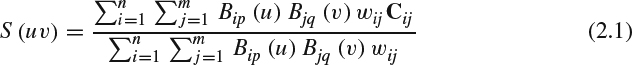
The refinement rule decides how to subdivide the original polygonal meshes. On the one hand, the vertex insertion scheme inserts three new vertices into each triangle as shown in Figure 2.11 and splits the triangle into four subfaces. The inserted vertices are then repositioned according to the refinement scheme.

On the other hand, the corner cutting scheme inserts extra vertices into each edge and the position of the inserted vertex is updated according to the subdivision scheme. Then the original vertices are removed and the connections of all inserted vertices are reconstructed accordingly. Figure 2.12 shows a simple example.

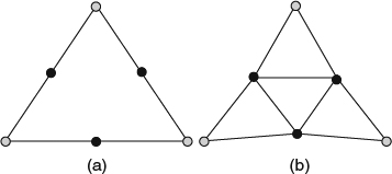
Figure 2.11 (a) The relative positions to the original three vertices drawn as gray dots and the insertion vertices drawn as black dots. (b) The result after applying the subdivision scheme to all inserted vertices.

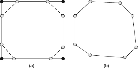
Figure 2.12 (a) The relative positions to the original vertices drawn as black dots and the insertion vertices drawn as gray dots. (b) The result after applying the subdivision scheme to all inserted vertices.

Figure 2.13 (a) An example result after applying the interpolation scheme. (b) An example result after applying the approximate scheme. The black dots represent the original vertices and the gray dots represent the new inserted vertices.

Refinement schemes compute the position and other properties of the newly inserted vertices. Approximating schemes mean that the limited surface after subdivision is only an approximation to the initial mesh, that is, after subdivision, the newly generated control points are not on the limited surface (see Figure 2.13b). Interpolating schemes mean that after subdivision the control points of the original mesh and the new generated control points are interpolated on the limited surface (see Figure 2.13a). Interpolating schemes provide the advantage of controlling the limit of subdivision in a more intuitive way and the approximating scheme can provide a higher quality of surface in fewer iterations of subdivision. For example, the loop subdivision scheme [49] uses vertex insertion and subdivides the triangular meshes using an approximating scheme. The main advantage of subdivision schemes is the smoothness, even with irregular settings [51], and Stam [45] proves that the limit of subdivision can be computed mathematically without explicitly applying subdivision recursion.

Another advantage of subdivision is to provide a method to build a multi-resolution mesh pyramid similar to the concept of the image pyramid. The pyramid provides the freedom to coarsen a given mesh and then refine it later to recover exactly the same mesh with the same connectivity, geometry, and parameterization. The coarsening process is equal to reversing the subdivision process, that is, repeatedly smoothing and downsampling. This is achieved by using an intermediate representation above the current representation in the subdivision hierarchy. Zorin et al. [52] and Lee et al. [53] propose that the geometrical information lost due to smoothing and downsampling is encoded into the subdivision process using the difference as detail offsets. The lost details can be recovered smoothly at any time through the subdivision process and the detail is independent of the others. The detailed mesh can be recovered from the coarse mesh by repeatedly subdividing the coarse mesh to add the detail. This also automatically provides a mechanism for progressive transmission and rendering [54, 55].

Note that since subdivision representations provide the guarantee of smoothness, they must deal with irregular meshes. Generally, the subdivision schemes divide vertices into two categories: regular and extraordinary. Extraordinary vertices are identified as vertices whose valence is other than six for the triangular case and four for the quadrilateral case. In order to guarantee smoothness, there will be a different refinement scheme for extraordinary vertices and the scheme generally depends on the vertices' valences such as [47].

2.2.1.10 Subdivision Construction

Subdivision is first developed because of the need in modeling, animation, and mechanical applications. Therefore, manual construction by a user is the main source of subdivision surfaces. The construction starts from creation of the base mesh using animation or modeling software and then a set of user interfaces is also provided to the users to set up constraints and select subdivision schemes and parameters to create the desired surface.

2.2.1.11 Subdivision Compression and Encoding for Transmission

The subdivision is constructed from a base mesh using a refinement scheme iteratively to subdivide the base mesh to the desired resolution, and thus the transmission of the subdivision can be done by sending the base mesh and the choice of refinement scheme and its associated parameters. Then the refinement of the base mesh to the desired resolution can be achieved in the receiver side. If necessary, the base mesh can be compressed one step further to minimize the amount of data transferred. According to the discussion in previous paragraph, multi-resolution analysis also allows the construction of an efficient progressive representation which encodes the original mesh with a coarse mesh and a sequence of wavelet coefficients which express the detailed offsets between successive levels. Therefore progressivity is supported naturally.

2.2.1.12 Subdivision Rendering

Generally, to synthesize a view of a subdivision object, the representation must first be transformed to a polygonal mesh at the desired resolution. Then the local illumination and global illumination scheme can be applied to generate the result.

2.2.2 Point Based Representation

Meshes represent the surfaces enclosing the objects. The information needed for a polygonal representation is generally large and complex. Thus, an efficient representation is proposed to only record sample points on the surface with the surface properties such as normal and material information. The representation is called point-based modeling including surface points [6, 56], particles [57], or surfels [4] which denote dimensionless space points. Figure 2.14a shows an example of point-based representations of the main building of Chiang Kai-shek Memorial Hall in Taipei.

The representations use simpler display primitives for surface representations. This set of points sampled from the surface contains no topology or connectivity information. In other words the set of points does not have a fixed continuity class nor are they limited to a certain topology as other surface representations. Hence, they can represent any shape with arbitrary topology and complexity. Point-based modeling was first proposed by Levoy et al. [6] to represent those phenomena that are difficult to model with polygons, such as smoke, fire, and water. With the recent advances in scanning technologies, the scanned 3D polygonal meshes can approximate real world objects to high accuracy but their triangle counts are huge and become processing bottlenecks with current graphics technology. Thus, point-based representation has regained attention recently. In addition, Pixar also proposed extending the point-based idea for micropolygons to accelerate the rendering process needed in animation production. This is because rendering a large number of triangles realistically becomes a huge issue in terms of its inefficiency. The projected size of a primitive in a highly detailed complex polygonal model onto the image plane during the rendering process is often smaller than the size of a pixel in the screen image. At this moment, the rasterization of polygonal meshes becomes unnecessarily costly. Therefore rendering individual points is more efficient in this situation.

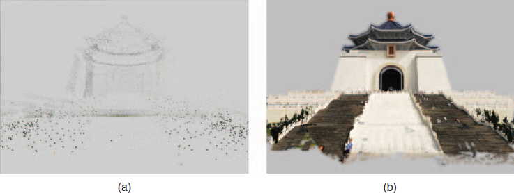
Figure 2.14 (a) A set of point samples of the main building in Chiang Kai-shek Memorial Hall. (b) The splatting algorithm is applied to render the point samples of the main building.

2.2.3 Point Based Construction

3D scanners are popular for surface-based representations. Many scanners first probe the object to create a set of sample points on the object surface and then a reconstruction method is applied. The set of sample points can be used as the point-based representation of the object. Another method creates a set of surface points by sampling a surface representation. The most crucial problem in sampling is how to distribute the sample points on the surface. For example, each patch can have a uniform number of samples or a number of samples proportional to its area or according to its curvature, and so on. Then the samples in each patch are distributed uniformly in the 2D space. Generally, the distribution scheme can be adjusted according to the needs of application.

2.2.4 Point Based Compression and Encoding for Transmission

Generally, point-based modeling can be more efficient with regard to storage and memory in the process of progressive modeling when compared to polygonal meshes because point-based modeling only needs the information related to samples but need not store the extra structural information such as connectivity. However, low-resolution approximations of point sets do not generally produce realistic rendering results and easily generate holes in the process. Therefore, progressivity is important for adjusting resolution for different displays and different transmission speeds. The first idea that comes to mind is to apply filtering techniques in a similar manner to the construction of image pyramids. Thus, the point set sampled on a regular grid can easily support progressive transmission/visualization and LoD scalability. Thus Yemez et al. [58, 59] proposed a progressive point-based modeling method based on an octree volumetric structure. Their method works as follows: the method first voxelizes the surface in octree volumetric representation and then hierarchical point sets are uniformly sampled on the surface according to the hierarchical voxel in the octree structure which will be discussed later. With the octree hierarchical structure, the samples can also be encoded in a similar hierarchical order and the viewer can reconstruct the surface information progressively.

Spherical hierarchy is another type of progressive point-based modeling and the visualization of the point set is rendered using splatting as discussed below. The algorithm uses different sizes of spheres to represent the hierarchy and the region enclosed by each volume. All those points located in the sphere belong to the same node and thus the algorithm can construct the tree structure, too. Since splatting is the main rendering method and will be discussed in the next section, the rendering technique allows the progressive transmission to render the point sets in different levels with different parameters. There are several other progressive schemes proposed after that. All these are based on hierarchical data structures [7, 58, 60, 61].

2.2.5 Point Based Rendering: Splatting

The simplest way to render the point-based representation is to reconstruct the polygonal surface as mentioned in the construction section of polygonal meshes. And then the global illumination and local illumination algorithms for polygonal meshes can be used to synthesize the view.

There is another group of methods called splatting which is carefully designed to achieve high visual quality at a speed of millions of points per second without the need for special hardware support [4, 7, 62–64] (see Figure 2.14b). Splatting renders a point using a small oriented tangential patch, and the shape and size of the patch can vary according to the design of the algorithms and the local density of points. The shape and size of the patch defining the kernel function of reconstruction. The shading or color of the patch is the original sampled color modulated by the kernel function. The kernel function can be a Gaussian function or non-Gaussian kernels can be used [65]. The choice of the kernel function is basically the trade-off between rendering quality and performance. One must note that when the points sampled in the object space are projected onto the image space, the projected points do not coincide with the regular grid of the image coordinate. As a result, if the projected process is not handled properly, visual artifacts such as aliasing, undersampling, and holes might appear. Gaussian circular splatting usually performs well. Other more sophisticated non-Gaussian kernels could also be used at the cost of an increase in rendering time [65]. Even without special hardware support, current splatting techniques can achieve very high quality when rendering point-based surface models at a speed of millions of points per second.

2.2.6 Volumetric Representation

A real world object always contains a volume. Thus, the general representation should be constructed from this concept. This representation refers to parameterizing the reconstruction volume in the world reference frame. The fundamental representation is to use a unit volume called a voxel which is defined in a regular grid in the world frame. In other words a voxel corresponds to the smallest representable amount of space [66]. This is similar to the pixel which is used as a basic unit in 2D image space to represent the information in an image. The fundamental information in a voxel encodes the existence of the object which records whether the voxel is inside or outside a valid object. Empty voxels are typically not associated with any information other than a Boolean flag indicating that they are vacant. In addition, the data associated with the objects, such as color, normal, and transmission index, can also be added into each voxel. Since the voxel records the existence and object attributes, the resolution of the voxel also determines the precision of the representation. Figure 2.15 shows a teapot represented by a set of voxels. Generally, straightforward implementation of a voxel space is through a volume buffer [9] or cuberille [67] which employs a 3D array of cubic cells.

Volumetric representations are good structures for multi-view stereo techniques which reconstruct a 3D scene from multiple images taken simultaneously from different viewpoints. The representations are valuable to provide a common reference framework for the images taken from multiple viewpoints [68–70]. In addition, they also include neighborhood information. In other words, the representation provides direct access to neighboring voxels. This is efficient for the computation of stereo algorithms such as space carving [71] and voxel coloring [72] approaches, where the reconstruction result is obtained implicitly by detecting the empty voxels. The representation also can help compute local geometric properties (e.g., curvature [73]), as well as for noise-filtering of the reconstruction results.

2.2.7 Volumetric Construction

There are mainly three different methods to generate volumetric data: 3D object or medical scanning (such as CT and MRI), physical simulation, and voxelization, that is, transformation from a polygonal mesh. The first category creates the 3D content via the depth-image-based representations. The second category is the product of physical simulation for generating animation or mechanical design for fluid such as smoke, water, and fire as discussed in the previous animation section. The third is to transform a polygonal mesh into a volumetric representation and the procedure is called voxelization. Kaufman et al. [74] proposed the first voxelization algorithm. Generally, volumetric data stores properties of an object in a set of regular 3D grids. Voxelization strategies can be classified based on how to describe the existence of a model as surface voxelization [75–77] which uses the existence of a voxel to describe the boundary and solid voxelization [78–80] which describes the existence of the boundary and interior of the entire model. Another common classification is based on how the existence of a voxel is represented and can be described as binary [81–83] and non binary [75, 80, 83–87] voxelization approaches. The latter can be further divided into filtered voxelization [80, 87], multivalued voxelization [83, 84], object identification voxelization [75] and distance transform [85, 86]. A large amount of previous work focuses on the sampling theory involved in voxelization and rendering to generate high rendering quality by introducing well-defined filters. Thanks to the advance in GPU technology. With its powerful flexibility and programmability, real-time GPU voxelization becomes possible. Chen [88] presented a slicing-based voxelization algorithm to slice the underlying model in the frame buffer by setting appropriate clipping planes in each pass and extracting each slice of the model to form a volumetric representation. There are later several improvements [81–83, 89–92] proposed to enhance the computation efficiency and enrich the rendering effects.

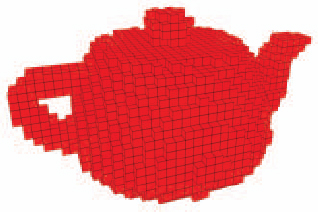
Figure 2.15 A teapot represented with voxels of a uniform size.

2.2.8 Volumetric Compression and Encoding for Transmission

Although the unit-sized volumetric representation can approximate any object to any desired accuracy, it might be quite memory-inefficient in several conditions. One condition is where the objects only occupy a small portion of the world. The objects contain complex details and thus the size of the voxel for representing the detail needs to be small, that is, the required number of voxels to represent the world is huge. The representation wastes a large amount of memory for empty space. If possible, a representation should use a large volume to represent the major part of the object and a small volume to represent the detailed part of the object. A common implementation of the above idea is called an octree [93]. Their idea starts from a coarse resolution, and the coarse representation is used to detect the large empty regions and large occupied regions. Then for those regions with mixed occupied and empty regions, the volume is subdivided into eight parts of equal size. The process recursively subdivide volumes into eight parts with an equal size and terminates at a predefined resolution. The proper data structure to represent this concept is a tree that grows in depth and whose nodes correspond to occupied voxels. Octrees can exhibit greater memory efficiency over uniform-sized voxel representation and provide the advantage of both data compression and ease of implementation. At the same time, the structure also provides progressivity by first sending the coarse structure in the top levels and then progressively sending the details in the lower levels.

Because of the compression and progressivity, there are several works proposed to improve the limitation of the original octree methods. These researches include linear octrees [94], PM-octrees [95], kD-trees [96], and interval trees [97]. Conceptually, the kD-tree, a binary space-partitioning tree, is similar to the octree except that each subdivision is binary and segments the volume by a plane of arbitrary orientation. The subdivision also terminates at a predetermined threshold of spatial resolution or height. This representation can provide better memory efficiency than unit-volume representations and better flexibility than octrees. However, the limitation is that the representation is not compatible with a regular parameterization which facilitates transmission and rendering. The compression and progressivity of volumetric representations is still an active research topic.

2.2.9 Volumetric Rendering

The main advantage of volumetric representations is their linear access time, and this property makes rendering new views efficiently and the rendering cost is independent of the complexity of the object. There are already GPU-based Z-buffer rendering algorithms [46] for synthesizing new views from volumetric representations.

Furthermore, volumetric representations can be transformed to meshes first and then the meshes are rendered with the graphics pipeline or global illumination algorithms. The easiest way to render a volumetric representation is to render each voxel as a cube. The polygonal cubes are rendered with a graphics pipeline but the rendering results for those cubes which are close to the viewpoint are generally not smooth and cause poor visualization. Instead of using polygonal cubes, polygonal meshes transformed from volumetric representations can produce smoother result and are the designed primitives for the commodity graphics architecture. Therefore, there are researches such as the marching cube [98] to generate better polygonal meshes from volumetric representations in more efficient ways. However, the resulting meshes are not optimized for memory usage, and geometrical structure is still shaped as an arrangement of cubes. This causes undesired artifacts in the rendering results.

When a light ray passes through a medium, the energy of the ray is absorbed by the medium along the path. Ray marching is a volume rendering algorithm built based on this concept. The ray casting process in ray marching is illustrated in Figure 2.16. When rendering a view, the algorithm shoots out a ray through the center of each pixel. The ray traverses through several voxels and the opacity and color of the voxel are accumulated to get the final color and opacity as follows:

where C and A are the color and opacity of the pixel, C_i and A_i are the color and opacity of the voxel i along the ray path, and N is the total number of voxels along the ray path. The contribution of the color from the voxel is weighted with the transparency product; in other words, those voxels that show up later in the path will contribute little. When the ray shoots out of the volume or the transparency product reach zero, the accumulation is finished. A view can be synthesized by tracing all view rays as described previously.

There are more volume rendering techniques. Interested readers could refer to [37] for more details.

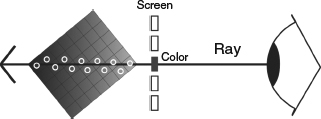
Figure 2.16 Schematic diagram of volume ray casting. A ray is cast from the eye passing through a pixel. The ray will continue to traverse through the object, and the color and transparency of voxels along the path will be accumulated to compute the color of the pixel.