4.3 2D-to-3D Video Conversion

In Section 4.2.4, we demonstrated a practical automatic 2D-to-3D video conversion module in a low-power mobile phone system. In this section, we cover the wider scope of 2D-to-3D conversion technology. In general, 2D-to-3D conversion is to convert the current 2D video content in DVD/Blu-ray or other formats into a 3D format with depth sensation. The efforts can be classified into two categories:

• Real-time solution: it is typically connected to the back-end display, and the conversion is done before the output is rendered. Currently, almost all major TV companies have built real-time 2D-to-3D conversion systems in their 3DTVs, some are using their own proprietary technology, and others are using rdthird party vendors, for example, DDD with a technology called TriDef, and Sensio's technology.
• Off-line solution: it handles the conversion in a much finer way with user interaction. The following companies are well known in this area:
  • In-Three plans to re-release the converted 3D version of Star Wars.
  • IMAX has converted a few footages, such as Superman Returns.
  • 3DFusion has an off-line 2D-to-3D conversion solution (built on top of Philip's solution) for membership based services.
  • DDD claimed to have its proprietary offline conversion solutions.
  • Akira provides 2D-to-3D conversion and 3D content creations services for its customers.
  • Legend films, a San Diego based startup company, provides services for converting 2D films into stereoscopic 3D.

In general, the key component of this conversion technology lies in the generation of a depth map for the 2D image; the depth map is a 2D function that provides the depth value for each object point as a function of the image coordinates. If there is only one 2D image, also called the monocular case, then the depth map has to be derived from various depth cues, such as the linear perspective property of 3D scenes, the relationship between object surface structure and the rendered image brightness according to specific shading models, occlusion of objections, and so on. Otherwise, binocular or multi-ocular cases with two or more images are used to reconstruct the 3D scene. Typically these images are captured from slightly different viewpoints, thus the disparity can be utilized to recover the 3D object depth. Other depth cues also include the disparity over time due to motion, the degree of blurring or focus, and so on. In this section, we focus on the monocular cases, and will discuss the binocular or multi-ocular cases in Section 4.4.

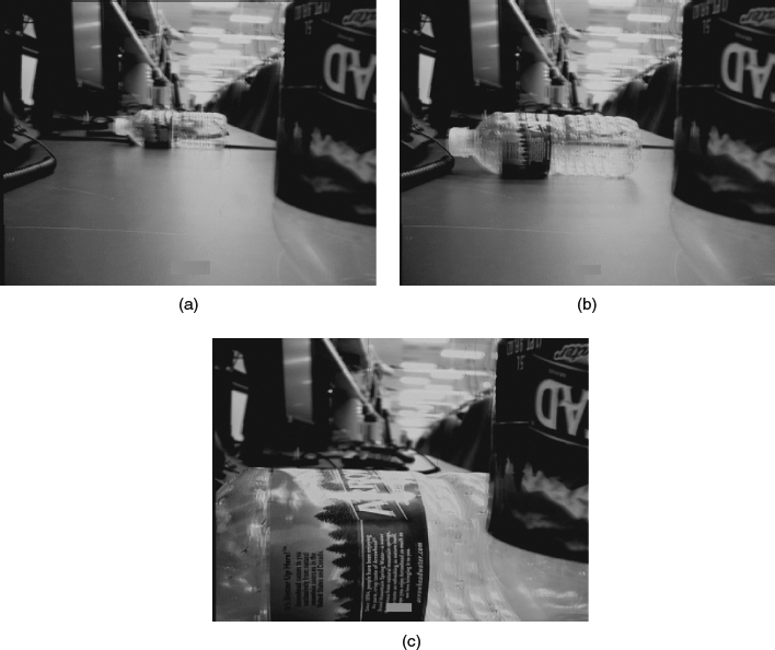
Figure 4.13 Examples of the resulting anaglyph video frames.

4.3.1 Automatic 2D-to-3D Conversion

In this section, we discuss methods in the field of automatic 2D-to-3D conversion. In other words, the human interaction is not considered in this scope and the images are captured in monocular devices. As mentioned above, the depth cues derivation is the focus of this conversion, and the source data has major impact on the approach to choose, for example, the derivation depth from a single image is the most challenging task due to the lack of information; if we have two or more images captured from the same camera (like a video clip), more useful information, like object motion, can be used in obtaining the depth map.

4.3.1.1 Depth Derivation from a Single Image

Depth from Geometric Cues

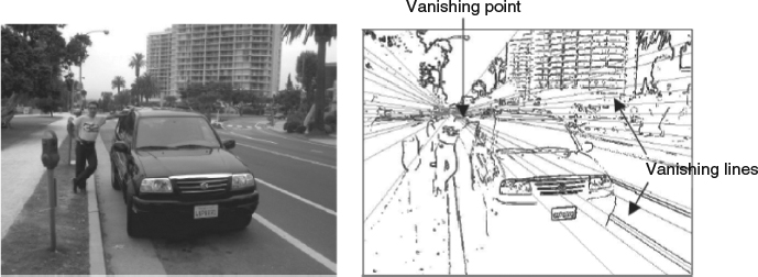
From a geometric point of view, many objects with long parallel edges, such as railroad tracks, share the same linear perspective property that the edges are converging with distance and eventually reach a vanishing point, which is typically the farthest position away from the camera. In [10] and [17], a gradient plane assignment approach was proposed to detect these edges and find interaction points, among which the interaction point with most edges passing through is determined as the vanishing point. The major lines close to the vanishing points are determined as the vanishing lines, and the lines form a few gradient planes which can map into certain structural models, for example, up case, down case, inside case, and so on. In the depth map generation process, the vanishing points are labeled with largest depth value, and the other points are labeled with depth interpolation according to the gradient structural model.

Depth from Planar Model

This approach assumes that all the 3D scenes are composed of planes or curved surfaces and thus can be approximated by simple models to reconstruct the 3D structure. For example, open sky can be modeled with a spherical surface; a scene consisted of a long-range view and flat ground of water can be represented by a model with a plane and a cylindrical surface, and so on. Once the planar model is determined, the relative depth map can be generated accordingly. As an example, a planar model can be used on indoor environment reconstruction, in which the indoor background is modeled with a few horizontal (floor or ceiling) and vertical (walls and doors) planes. To detect and extract the planes from the image, the wall borders and corners are first extracted with a Harris corner detector in the gradient map of the input image, then a filter-and-merge process is used to keep all meaningful segments which delimit the relevant planes of the scene.

Depth from Focus and Defocus

This approach relies on the blurriness of different regions in the image, that is, the objects in-focus are typically not blurred while the blurriness will be observed on the objects out-of-focus. In this way, the objects are distinguished as foreground objects and background objects, which also gives an indication of the depth level of the objects. In [18], a relationship between the depth and blurriness is proposed as:

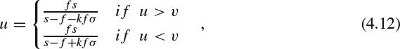
where u is the depth, ν is the distance between the lens and the position of the perfect focus, σ is the blur radius, s, f, and k are camera parameters, in which s is the distance between the lens and the image plane, f is the focal length of the lens, and k is a constant determined by the camera lens configuration. Clearly, the depth can be obtained once the blur radius is determined, as the camera parameters s, f, and k can be obtained from camera calibration.

As mentioned in Section 4.1.4, a depth from focus approach is proposed for a low-power mobile device [15]. In the proposal, the autofocusing process of the device positions the lens through an entire focusing range and selects the focus position with a maximum focus value. Thus the device can create a block depth map automatically using statistics from the autofocusing step and in a second-stage generating an image depth map.

Depth from Shading

This approach uses the relationship between scene object surface geometry and the brightness of the image pixels. Clearly the scene object surfaces can be described as a set of 3D points (x, y, Z(x, y)), and thus the surface slopes at this point are and . By assuming a known light source with orthographic projection mode, and a known reflectance model (for example Lambertian), the relationship between the estimated reflectance map and the surface slopes can be formalized. By adding smoothness constraint, the problem can be converted into a minimum energy function and thus eventually can derive the depth map. In [19], a shape from shading approach is proposed by using finite-element theory.

4.3.1.2 Depth Derivation from an Image Sequence

Depth from Motion

This is also called structure from motion (SfM), because the purpose is to extract the 3D structure and the camera movement from an image sequence; typically we assume that the objects in the scene do not deform and the movements are linear. The 2D velocity vectors of each image points, due to the relative motion between the viewing camera and the observed scene are referred to as the motion field, which can be calculated via the object's translational velocity vector, the camera's angular velocity, and perspective projection transformation to map the 3D space to 2D. Once the motion field can be reconstructed from the image sequence, the 3D structure reconstruction can be done in the similar way as the binocular case (which will be discussed in Section 4.4). The motion field becomes almost equivalent to a stereo disparity map if the spatial and temporal variances between the consecutive images are sufficiently small.

The motion field estimation is typically done via optical flow based approach or feature based approach. The key point of optical flow is assuming that the apparent brightness of a 3D object is constant, thus the spatial and temporal derivatives of image brightness for a small piece on the same object are calculated to maintain the image brightness constancy equation:

where the image brightness is represented as a function of image coordinates and the time, and the partial differentiation of E with respect to the spatial (also called gradient) and time are used to represent the motion velocity of the image point in space and time.

Feature based motion field estimation generates sparse depth maps by tracking separate features in the image sequence. A typical approach in this category is the Kalman filter, which is a recursive algorithm that estimates the position and uncertainty of moving feature points in the subsequent frames.

Hybrid Approach

Hybrid approach means to use a combination of depth cues to detect the depth map, for example, considering combined cues of motion based and focus cues; the motion based cue is used to detect the depth ordinals of the regions in each frame, and a focusing algorithm is applied to estimate the depth value for each pixel in the region. In [20], three different cues were used to obtain the final depth map. Firstly, a blur estimation stage is applied to generate a blur map for the whole frame to find foreground (unblurred region) and background (blurred region); then an optical flow algorithm is used to detect the occlusion in each consecutive frames; after that, a depth ordinal method is adopted to detect the spatial relation according to occlusion information; finally a disparity map is constructed using the blur map and the depth ordinal information.

4.3.1.3 Complexity Adaptive 3D Conversion Algorithm

In this section, we demonstrate a complexity adaptive algorithm for automatic 2D-to-3D image and video conversion. First of all, a novel image classification approach is proposed that can classify an image into flat or non-flat type, which reduces the computational complexity for processing flat image, and helps to reduce possible outliers in the image depth map generation. Then a novel complexity adaptive algorithm was proposed for image depth map estimation, which is a rule based approach that uses object segmentation to help adjust the depth of pixels belonging to the same object, and use temporal depth smoothing to avoid the visual discomfort caused by segmentation errors. The complexity is adaptive in the sense that the procedure can be simplified to trade estimation accuracy with processing speed.

The focus of this work is to convert a 2D image sequence into a 3D image sequence, while the other issues such as the bit stream format of the input images (i.e., compressed or raw data) and the display methods for the output video are not within the scope. Without loss of generality, we assume that the images for processing are in the YUV or RGB format, and the outputs are left and right views.

We propose a complexity adaptive depth-based image conversion algorithm, and its system architecture is shown in Figure 4.14. When an image is coming in, a color-based image analysis approach is used to detect if the image represents a flat scene. If so, then both views would be identical and thus the original image can be used for the view. Otherwise, a rule based image pixel depth estimation method is used to assign approximated depth for each pixel. If there are no low-complexity constraints, the depths are adjusted by using object segmentation so that the pixels representing the same object can have similar depth values. Otherwise, this step is skipped or partially skipped to trade accuracy with speed. The generated depth map is processed by an algorithm to automatically generate the stereo image pairs representing the left and right views.

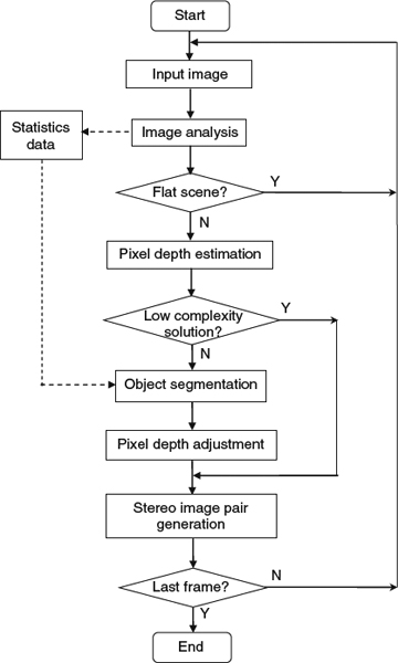
Figure 4.14 System architecture of the complexity adaptive depth-based image conversion algorithm.

In the following text, we demonstrate a novel approach to estimate depth for each pixel in the image. It is evident that the stereo views can be generated by a monoscopic image and its associated depth map. Generally, our approach is based on a set of rules obtained from observations. As an example, for outdoor images the upper side has a good chance of representing the sky, and the ground is normally positioned at the bottom of the image. This matches the observations that there is a tendency that the center and bottom parts of the image are nearer than the upper sides in general images.

Figure 4.15 Examples of zoomed images.

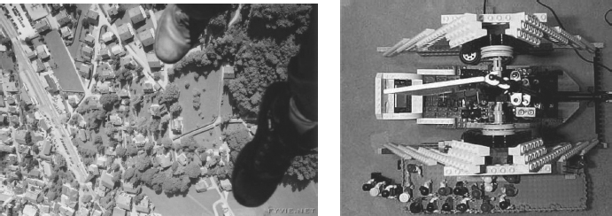
Figure 4.16 Examples of view-from-above with a 90° camera elevation angle.

We first classify the images into flat image and non-flat image. The former class contains almost no depth information and thus no depth estimation is needed. We observe that there are two kinds of images that are potentially flat images: (1) zoomed images as shown in Figure 4.15, where the pixel depth differences in the image are visually negligible due to the zooming effect; (2) images corresponding to view-from-above (or below) with a 90° camera elevation angle as shown in Figure 4.16.

In addition, we observe that views with elevation angles less than 90°, as shown in Figures 4.17 and 4.18, contain sufficient depth information. Moreover, the depth information from these views is easier to extract than from the views with a 0° elevation angle because the view angle increases the depth perception.

In this work, we assume that the videos for processing are carefully produced, thus the visual discomfort has been limited to a low probability. Therefore, it would be valid to assume that the occurrences of upside down images, and view-from-above (or below) with a 90° camera elevation angle, in the video are negligible. We assume that the camera orientation is normally aligned with our normal perception.

Since zoom-in and zoom-out are commonly used camera operations in video capture, in order to detect the flat images, we need to be able to automatically detect the zoomed frames. Ideally for zoom in frames, the “blow out” motion pattern would happen in motion estimation. In other words, the motion vectors of the macroblocks will point outward from the center of the zoom operation with vector length proportional to the distance from the center of the zoom operation. However, the noise in the frames might cause inaccurate motion estimation and thus false detection, plus motion estimation is quite computationally intensive for low-complexity applications. In this work, we propose a color-based zoomed image detection algorithm.

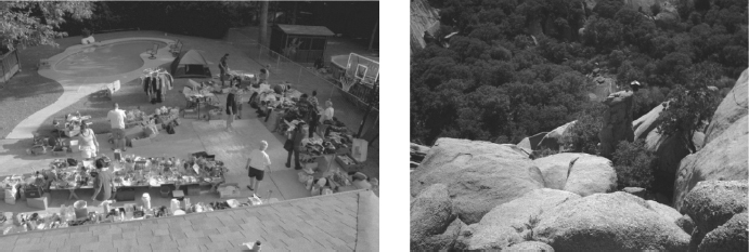
Figure 4.17 Examples of view-from-above.

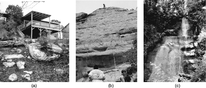
Figure 4.18 Examples of view-from-below.

We observe that in most video sequences the camera zoom operation follows the sequence of zoom-in → stay → zoom-out, or zoom-in → stay → scene change, so that the zoomed image can be detected by color-histogram change. Let us denote by n the index of the current frame f_n, T_n the zooming type of the current image (T_n = 1 represents the zoomed image, otherwise T_n = 0), V_n the variance of the current image, H_n(C_n,m) the 32-bin color histogram and C_n,m the color with sorted histogram (i.e., C_n,0 the color with the highest histogram), and S(f_n−1, f_n) the scene similarity between two frames f_n−1 and f_n(S(f_n−1, f_n) = 1 means there is a scene change). S(f_n−1, f_n) is defined as follows:

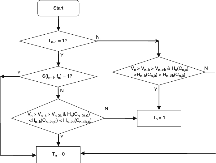
Figure 4.19 Logic for determining zoomed image.

where

and Th is a threshold to detect the image similarity.

The zoomed image can be detected by the logic shown in Figure 4.19. Clearly, if the previous frame is a zoomed image and the current frame is not a scene change, we need to detect if the camera is zooming out. The zooming out scenario can be determined by the gradual increasing of image variation and the gradual deceasing of the percentage of certain colors (primary color components of the previous frame) in the recent frames. Similarly, if the previous frame is not a zoomed image, we need to detect if the camera is zooming in. In Figure 4.19, the value k is a constant that determined by the frame-rate and normal zooming speed. For a 30-frame second per video clip, k = 10 could be a reasonable setting for the proposed algorithm.

Then we handle the non-flat images. It is important to realize that in this application, our purpose is not to recover the actual depth of the image pixels, but to generate or estimate an image depth map to enhance the 3D effect of the original image. Our approach is based on two fundamental assumptions: First, the scene is composed of a number of objects, and the pixels corresponding to the same object have closer depth values, and their differences can be negligible. Second, for most non-flat images, the depth of the objects decreases from the top to the bottom. There are some counter-examples, such as indoor scenes as shown in Figure 4.20a, and cases when occlusion occurs, but to detect such scenes is extremely difficult and time-consuming and there are so far no low-complexity solutions available. In general, we observe that the assumptions are valid for most video clips, and the counter-examples do not have significant impact on the visual effect of the generated 3D images.

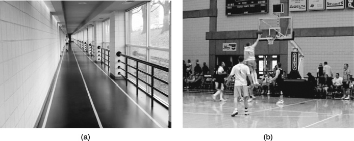
Figure 4.20 Example of indoor images. (a) Case that is contrary to the assumption. (b) Case that agrees with the assumption.

Initially, we assign each pixel a depth value which is proportional to its vertical coordinate value. After that, we adjust the depth map based on the results of the object segmentation. As shown in Figure 4.21, to reduce the computational complexity we could select only a portion of the image for segmentation when it is necessary. Since the center and bottom regions normally correspond to closer objects that are more visually sensitive, we choose these regions as the aea for segmentation. In this work, we use a complexity adaptive scheme, that is, when a higher complexity solution is acceptable, we apply motion estimation to get motion information and use both color and motion information for object segmentation. When a medium complexity solution is expected, we only use color information for segmentation. For real-time applications or when a low complexity solution is expected, we skip the segmentation operations to avoid heavy computation. We assume that there is a feedback channel from the system controller to inform this application of the current status of the system, for example resource allocation and CPU usage, so that our proposed system can choose the solution adaptively, based on the image complexity.

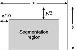
Figure 4.21 The selected segmentation region.

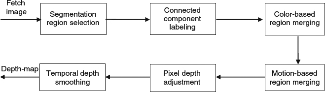
Figure 4.22 Primary flow of image depth map adjustment.

In Figure 4.22, more details of the depth map adjustment are shown. After the segmentation region is selected, we use a connected component labeling approach to divide the image into a number of small connected regions where the pixels inside the same region have similar color intensity. Then a color-based region merging algorithm is used to merge these small regions into bigger regions if any neighboring subregions have close mean color intensity. Motion information (if available) is used further to merge regions moving in the similar direction into bigger objects. After the segmentation steps are completed, we adjust the pixel depth for each object, and assign the depth of each pixel inside an object to be the minimum depth of the pixels in the object. Finally, a temporal depth smoothing process is needed to avoid sharp depth change between adjacent frames. The motivation behind this is that in general the frame rate of video clips is high enough so that the objects in the scene does not move very fast in depth except for some occlusion cases. Let us denote by d_n−1(i, j) and d_n(i, j) the depth of pixel (i, j) in the (n−1)th and nth frame, so the d_n(i, j) is adjusted as follows:

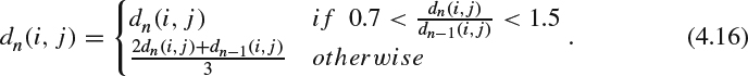
An example of the generated depth map is shown in Figure 4.23, where b is the estimated depth map corresponding to the original image shown in Figure 4.23a. In the map, the lighter area corresponds to the further objects, and the darker area corresponds to the closer objects. Clearly, the results indicate that the proposed algorithm is capable of approximately distinguishing further objects from closer ones, although some misclassified objects exist due to the lack of semantic information for better segmentation.

4.3.2 Interactive 2D-to-3D Conversion

The interactive 2D-to-3D conversion is also called offline conversion, as human interaction is required in certain stages of the process flow, which could be in terms of object segmentation, object selection, object shape or depth adjustment, object occlusion order specification, and so on. In the next section, we showcase a real scenario that demonstrates many interactive components in a 3D conversion system.

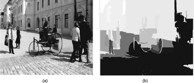
Figure 4.23 Example of the generated depth map. (a) Original image. (b) Estimated depth map (the darker the smaller depth).

4.3.3 Showcase of 3D Conversion System Design

In this section, we showcase an example 2D-to-3D conversion system, which is a novel hybrid design that contains both a real-time and an offline conversation system; in other words, the framework uses an interactive 2D-to-3D conversion environment (i3DV) to train an automatic 2D-to-3D conversion solution (a3DC); the interactive environment provides built-in intelligent processing toolkits and friendly user-interfaces to reduce the user interaction and supervision to a minimum, and at the same time it enhances a knowledge base to support the training of the a3DC. The automatic solution, a3DC, starts with a very simple gravity-based depth generation algorithm, with the new rules generated and adjusted by the knowledge base, then the a3DC is able to incorporate the rules and consequent execution procedures into the system to enhance the accuracy of the generated 3D views. To the best of our knowledge, this is the first framework that has been proposed in literature to use a training system for the automatic creation of 3D video content.

Clearly, this framework is very useful for media service providers, where the content for broadcast or delivery are controlled. The media server can start the services of the 3D movie (converted from a 2D content) by creating content using the i3DV; then with more and more titles being generated and the i3DV knowledge base expanding to a mature degree, the a3DC would become more accurate and eventually could significantly reduce the workload and user interactions of i3DV. For similar reasons, the framework would be useful for the content creator and even for TV vendors who have portal services.

As you can imagine, to implement such a framework is not a trivial task. We list below the major challenges and difficulties to consider:

For i3DTV, we need:

• an intuitive, efficient and powerful user interface to support segmented object boundary correction, object selection, scene/object depth specification and adjustment, 3D effect preview, etc.,
• a built-in video shot segmentation algorithm to simplify the video editing and frame/object management tasks,
• a built-in temporal object tracking/management algorithm to guarantee the temporal coherence in 3D depth and to reduce user interaction,
• a built-in scene geometric structure detection algorithm to help the user to determine depth hierarchy of the scene (including the vanish point/lines) with few interactions,
• a built-in interactive (or semiautomatic) object segmentation algorithm to speed up user interactivity,
• (advanced/optional) a built-in scene/object classification model/database and training system (with hand-labeling) to enhance the built-in knowledge base for semantic scene/object recognition (with various poses and even in deformed shapes),
• a depth-based image rendering algorithm to generate left/right views from a depth+2D image input,
• a built-in objective 3D perceptual visual quality measurement mechanism to provide feedback to the end user for the derived 3D content.

  For a3DC, we need:

• a user interface to specify the computational complexity expectation and customize the adopted algorithms and processing modules,
• a plug-in interface to download hinting information from the i3DV knowledge base to enhance the system accuracy,
• a built-in automatic object segmentation algorithm,
• a built-in rule based scene/object depth hierarchy estimation scheme,
• a depth based image rendering algorithm to generate left/right views from a depth+2D image input.

As an interactive system, the i3DV's architecture design (shown in Figure 4.24) follows the model-view-controller (MVC) architectural pattern, in which the system consists of three major components that may run at different platform (or machines):

• Model: the information reflects the application's operations. As shown in Figure 4.24, it is the i3DV internal data.
• View: the rendered format for user interaction. As shown in Figure 4.24, it is the 2D or 3D video preview window for the user's further interaction.
• Controller: the agent to process user interactions and change the model accordingly. In this system, the event handler plays this role.

In i3DV, to speed up the user interactivities, a set of built-in toolkits are supported for processing the model; these include automatic key frame selection and scene geometry structure detection. As shown in Figure 4.24, there are six parallel threads running simultaneously:

• Video structure management: the automatic key frame selection module initially analyzes the original video to detect the scene change, frames with geometry structure change, or new objects appearing, and thus break the video frames into a few chunks starting with key frames. The user can review the break points and adjust the locations or increase/decrease key frames. In principle, a significant portion of the user interactions are allocated for processing these key frames.

  

  Figure 4.24 The system architecture of i3DV.

  

  Figure 4.25 An example of scene geometry structure shown in [10]. Source: S. Battiato, S. Curti, M. L. Cascia, M. Tortora, and E. Scordato (2004) “Depth Map Generation by Image Classification”, in Proc. SPIE, Vol. 5302, pp. 95–104. Reproduced with permission from the author.

• Scene geometry structure management: the scene geometry structure detection module detects the orientation of the scene considering geometry factors, such as vanishing point and the vanishing line as shown in Figure 4.25. The orientation helps to expand the 2D image into 3D with depth direction. With user interaction, the scene geometry structure can be refined or adjusted to reflect natural perceptual feelings.

  

  Figure 4.26 An example of object classification shown in [21]. Source: J. Shotton, J. Winn, C. Rother, and A. Criminisi (2009) “TextonBoost for Image Understanding: Multi-class Object Recognition and Segmentation by Jointly Modeling Texture, Layout, and Context”, International Journal of Computer Vision, Vol. 81, No. 1.

• Semantic object management: the interactive object segmentation and tracking modules cut a set of foreground objects out of the image, and a few operations on the object can be conducted to refine the object boundary and to specify the depth information and the orientation of the object. Other than that, the object recognition and classification module would classify the object into a known class, for example, sky, water, or tiger (an example is shown in Figure 4.26), and the user can add labels to the object as well.
• Final or internal results preview: once the depth layer of the scene is specified or detected, the depth-based image rendering module can be called to generate the left/right view to be rendered in the 3D display. Also, the internal results – such as an object evolving along the time sequence or the chain of selected key frames – can be displayed as a sanity check.
• Visual quality control: a non-reference 3D quality evaluation module is deployed to generate a score to rate the perceptual quality of the converted 3D scene from the 2D image. The feedback is shown to the user so that they can refine the results.
• Semantic rules collection: a training system is available to learn the intelligence in scene orientation detection, object segmentation and object classification, and to refine a knowledge base for future usage in automatic 2D-to-3D conversion and other applications.

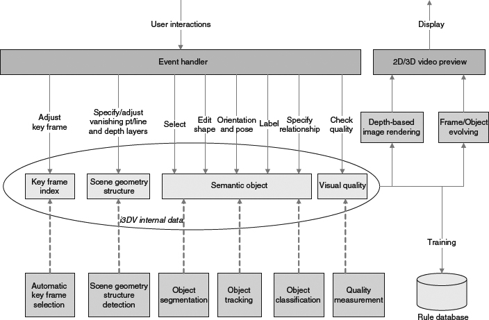
In the following text, we will focus on the visual data management and semantic rules collection parts, as others will be covered in other chapters of this book.

4.3.3.1 Visual Data Management

In i3DV, there are three threads of visual data management at different levels: video sequence level (video structure and key frame management), frame level (scene geometric structure management), and object level (object management). The management tasks include detecting or recognizing a component, adding/removing a component, selecting a component for editing and manipulation, and analyzing the component from user input and interaction.

Video Structure Management

Video structure analysis is important for i3DV as it differentiates the video frame into various hierarchical levels so that many frames that have significant similarity to their neighbors can use less user interaction for the depth map refinement work. Many video clips, such as newscast and sports video, exhibit characteristic content structure. There are lots of studies on the understanding of newscast video which take advantage of the spatial and temporal structure embedded in the clip. The spatial structure information includes the standardized scene layout of the anchor person, the separators between various sections, and so on, while the temporal structure information refers to the periodic appearances of the anchor person in the scene, which normally indicates the starting point of a piece of news. Similarly, sports video has well-defined temporal content structure, in which a long game is divided into smaller pieces, such as games, sets, or quarters, and there are fixed hierarchical structures for such sports. Also, there are certain conventions for camera work for each sports; for example, when a service is made in a tennis game, the scene is usually commutated with an overview of the field. In [22], tennis videos are analyzed with a hidden Markov model (HMM). The work first segments the player using dominant color and shape description features, and then uses the HMMs to identify the strokes in the video. In [23] and [24], soccer video structure is analyzed by using HMMs to model the two basic states of the game, “play” and “break”, so that the whole game is treated as switching between these two states. The color, motion and camera view features are used in their works; for example, the close-ups normally relate to break state while global views are classified for play. In [25], the stylistic elements, such as montages and mises en scène, of a movie are considered as messengers for video structure understanding. Typically, montage refers to the special effect in video editing that comprises different shots (a shot is the basic element in videos that represents the continuous frames recorded from the moment the camera is on to the moment it is off) to form the movie scenes, and it conveys temporal structure information, while the mise en scène relates to the spatial structure. In their work, statistical models are built for shot duration and activity, and a movie feature space consists of these two factors formed so that it is possible to classify the movies into different categories.

Key frame extraction (or video summary) is the technique of using a few key frames to represent the fundamental structure of a video story. Clustering techniques [26] are widely used in this area. In [27] an unsupervised clustering was proposed to group the frames into clusters based on the color histogram features in the HSV color space. The frames closest to the cluster centroids are chosen as the key frames. In [28] cluster validity analysis was applied to select the optimal number of clusters, and [29] uses graph modeling and optimization approaches to map the original problem into a graph theory problem, where a spatial–temporal dissimilarity function between key frames is defined, and thus by maximizing the total dissimilarity of the key frames a good content coverage of the video summary can be achieved.

Clearly, most of the works mentioned above are concentrated from the semantic point of view, while none of them considers 3D scenarios or the depth structure concept. In i3DV, a novel key frame extraction scheme is proposed that uses the 3D scene depth structure change as the major concern for shot boundary detection. This way, the classified non-key frames do not cause significant change in the scene depth structure, so that the depth map automatically generated from these frames (or derived from its preceding neighboring frame) needs less user interaction for refinement.

Scene Geometric Structure Estimation

Although quite a luxury to achieve, reconstructing scene geometric structure can significantly improve the accuracy of the depth map estimation. In [10] the linear perspective property is used for scene structure estimation, that is, in perspective viewing mode the parallel lines converge at a vanishing point, thus by detecting the vanishing points and lines, the projected far-to-near direction of the image can be obtained and thus the geometric structure can be derived. Then [30] proposes a stereoscopic image editing tool using the linear perspective property that was adopted in [10] for scene depth map estimation; the tool manually segments the objects into various layers and maps the depth to these objects before the 3D rendering process.

In i3DV, a novel scene geometric structure estimation approach is used based on semantic object classification and orientation analysis. The general image patterns are modeled thus the potential topological relationship between objects can be derived and thus the scene structure with the maximum probability is obtained.

Semantic Object Management

It is observed in [31] the semantic objects are the basic units for image understanding by our eyes and brains; in other words, these objects provide meaningful cues for finding the scene content. Furthermore, the interactions among semantic objects and the changes of their relative positions often produce strong depth sensation and stereo feelings for viewers. In this section, we discuss the following issues relating to object management in i3DV:

• how to cut an object out from its surrounding environment,
• how to describe the orientation and depth-directional thickness of an object,
• how to maintain a reasonable evolving path of an object crossing the time domain in a video sequence,
• how to describe the relative distances among objects,
• how to provide semantic meaning to an object.

Object Segmentation

Object segmentation [32], as a useful tool to separate the scene content into its constituent parts, has been widely studied in image/video processing, pattern recognition, and computer vision for the past several decades; however, so far there is no unified method that can detect all semantic objects [31] due to the fact that each object may have certain prior knowledge base for spatial/temporal pixel classification and processing, while different objects may have different characteristics. In recent years, much effort has been focused on interactive image segmentation; [33, 34], provide much better performance compared to the automatic algorithms.

In Figure 4.27, the user interaction as well as the results achieved by using various methods are compared and demonstrated. In the magic wand method [35], shown in 4.27a, the user specifies a few points inside the object region thus a region of connected pixels that covers these points based on color statistics would be segmented out. In the intelligent scissors method [36], the user traces the object boundary with the mouse, and in the meantime selects the minimum cost path from the current mouse position to the last clicked point when moving the mouse. In the Bayes matte [37] and knockout 2 [38] methods, the user specifies the masks (white mask for foreground and red mask for background) for a trimap which includes background, uncertain areas, and foreground. For the graph cut method [39], the user has a red brush to paint on the background region and a white brush to paint on the foreground region, then an energy minimization formulation based optimization process is trigged to conduct the segmentation. GrabCut [34] greatly simplifies the user interactions by only requiring the user to drag a rectangle loosely around an object and then the object would be extracted automatically. It extends the graph cut algorithm by iteratively optimizing the intermediate steps, which allows increased versatility of user interaction. For the cases that the initial user labeling is not sufficient to allow the entire segmentation to be completed automatically, the GrabCut would use the same user editing approach used in graph cut for further refinement. Figure 4.28 shows an example of such scenarios. The authors of [40] extend the framework to the video segmentation and make the user interactions in 3D video cube space instead of 2D image space. In [41], a new segmentation algorithm based on cellular automation is proposed, which provides an alternative direction to graph theory based methods.

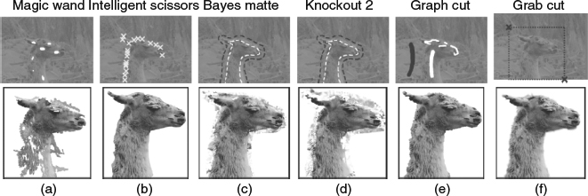
Figure 4.27 Comparision of various segmentation tools in [35]. Source: C. Rother, V. Kolmogorov, and A. Blake (2004) “GrabCut – interactive foreground extraction using iterated graph cuts,” in Proc. SIGGRAPH 2004, pp. 309–314.

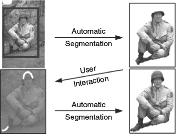
Figure 4.28 Further user editing process in GrabCut [35]. Source: C. Rother, V. Kolmogorov, and A. Blake (2004) “GrabCut – interactive foreground extraction using iterated graph cuts,” in Proc. SIGGRAPH 2004, pp. 309–314.

In i3DV, we extend the GrabCut method to 3D video space, and with motion estimation a 3D bounding pipe for an object can be derived from the 2D bounding box specified by the user, and with modest user interactions the object moving path in the 3D space can be extracted. The temporal cues in the 3D pipe make the 3D-GrabCut algorithm more accurate than the original GrabCut in 2D spaces.

Object Orientation and Thickness Specification

Once the object is segmented out, we need to estimate the depth of the object in the scene, thus the orientation and thickness of the object matters. In i3DV, the objects are classified into three categories:

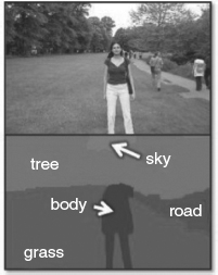
• very far objects, for which the depths can be set as a default large value and the thickness can be considered as zero; the tree and sky in Figure 4.26 are good examples for such objects,
• objects with significant thickness, for example, the grass and road in Figure 4.26,
• flat objects for which the thicknesses are negligible, for example, the body object in Figure 4.26.

Clearly the object orientation only matters for the objects with significant thickness, as shown in Figure 4.29, the user can specify the object orientation by linking the most far point of the object with the nearest point of the object (see the red dash arrow lines in Figure 4.29 to specify the orientations for grass and road objects), this way the orientation of the object is determined. This approach works with an assumption that the pixels in the same object aligned in the same horizontal line are in the same depth in the scene.

However, this assumption does not work for all scenarios; in which case, the far surface and the nearest surface of the object need to be specified. Figure 4.29 shows an example of such a scenario, where both near and far surfaces are specified with boundaries and a number of orientation directions in dashed lines are specified so that the remaining directions can be interpolated from the specified major ones.

Clearly with the specification of object orientation and thickness, the relative depths of all the pixels on the object can be easily derived.

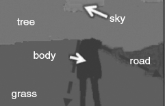
Figure 4.29 An example of object orientation specification.

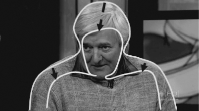
Figure 4.30 An example of object orientation specification.

Tracing Objects in the Time Domain

For many video clips, object tracing in the time domain is trivial if the object movement and transformation activities are not heavy and the camera viewpoint remains the same all the time. However, there are tough scenarios (see for example Figures 4.30 and 4.31) where the camera is in zoom in/out mode, which makes overall depth range of the scene change all the time as well as the sizes and positions of objects in the scene. For such cases, certain user interactions have to be made to ensure correct object tracing thus making the object depths/thicknesses consistent along the time domain.

Topological Relationship among Objects

In i3DV, a scene registration and object management scheme is adopted to maintain the consistency of the topological relationship among objects and between the object and the scene. For example, in Figure 4.29, the depth of the body object is the same as the nearest surface of the grass object, and the body feet are on the same horizontal line as the nearest boundary edge of the grass object. However, the same rule cannot be applied in Figure 4.30, where the depth of the wall (which is a flat object) should be larger than that of the most distant surface of the speaker object, although at the bottom of the image, their edges are on the same horizontal line. By assigning depth value to the object surfaces, the topological relationship among objects can be uniquely determined.

Object Classification and Labeling

In i3DV, the purposes of object classification are as follows:

• The scene geometric structure can be derived from the labeled object categories, thus the topological relationship among objects can be investigated from a semantic point of view.
• The scene composition pattern can be used for video structure analysis and frame management.
• Automatic object classification speeds up the user interaction for labeling.
• The user interactions for correcting the object classification can help in building and refining the backend object database for future applications.

Figure 4.31 An example of tough scenarios for object tracing.

So far there are many efforts in literature on object classification [21–42]. In [43], a limited number of datasets are trained to categorize small number of object classes, such as building, grass, tree, cow, sky, face, car, bicycle, and so on. Most methods are based on the textons or texton histograms; that is, the training images are convolved with a filter-bank to generate a set of filter responses, and these responses are clustered over the whole training set to result in high-dimensional space feature vectors, also called textons. Both [44, 45] aim to collect a much larger dataset of annotated images with web-based resources. First [44] pairs two random online users who view the same target image and try to make them read each other's mind and agree on an appropriate name for the target image as quickly as possible. This effort was very successful and it has collected over 10 million image captions with images randomly drawn from the web. Then [45] provides a web-based annotation tool called LabelMe (see Figure 4.32 for an example of its user interface), in which the user can annotate any object by clicking along its boundary and then indicating its identity. After sufficient annotations of a specific object class are obtained, a detector can be trained again and again from coarse to fine [46], and it can support the labeling process to become semi-automatic.

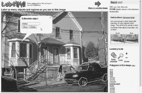
Figure 4.32 An example of LabelMe snapshot user interface. Source: B. C. Russell, A. Torralba, K. P. Murphy, W. T. Freeman (2008) “LabelMe: a database and web-based tool for image annotation”, International Journal of Computer Vision, pp.157–173, Volume 77, Numbers 1–3.

In i3DV, a quite similar approach is used for object classification and labeling: during the user interactions for object labeling, the object dataset is enlarged gradually and the algorithm training process is going on to refine the features to eventually reduce the user interaction frequency and thus make the object classification task more automatic.

4.3.3.2 Semantic Rules Collection

In this section, we demonstrate how i3DV helps in building the a3DC with all the semantic knowledge obtained from machine learning. Typically depending on the applications, the relationship between i3DV and a3DC follows either of the two models below:

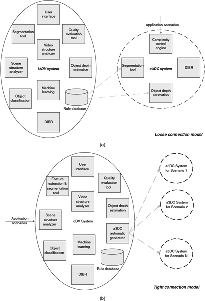
• Loose connection model: in which the a3DC is a well-established system that takes inputs (rules, heuristics, etc.) from i3DV's rule database. In this model, the a3DC can accelerate certain modules with hardware accelerators, while the rules provided by i3DV can improve its intelligence but is not an imperative condition, which gives more flexibility for a3DC implementation. Figure 4.33a shows the diagram of this model.
• Tight connection model: as shown in Figure 4.33b, in this model the a3DC systems are generated from i3DV according to the application scenarios, so the flexibility of a3DC implementation is reduced. Typically a3DC systems are automatically derived software solutions, as the i3DV is evolving with more and more video clips are processed and more user interactions are feed into the system. Consequently the performance of the a3DC system improves as the i3DV gets more mature.

In i3DV, a machine learning system is deployed to extract semantic rules for increasing automation of the system. Ideally the i3DV can achieve the following items of video understanding with the support of user interaction:

• objects are segmented from each other;
• objects are labeling with their category;

  

  Figure 4.33 Relationship between i3DV and a3DC. (a) Loose connection model for i3DV and a3DC. (b) Tight connection model for i3DV and a3DC.

• object orientation and thickness are labeled;
• object evolving procedures along the time domain are specified;
• scene constitution and semantic meanings are obtained with topological relationship among objects.

Theoretically these high-level semantic items are goals for a3DC to achieve, although they are not trivial at all. A practical approach is to use the low-level features, such as color, edge, texture, and so on, which are achievable in both a3DC and i3DV, as common platforms, and then use Bayes models to incorporate prior knowledge about the structure of the video content, to bridge the gap between low-level features and high-level semantics. Also, [25], [47], and [48] use the same concept in video understanding work. Typically the semantic scenes and events are modeled with a predefined statistical framework that supports an inference of unobservable concepts based on their relevance to the observable evidence. This way the high-level semantics may be inferred from the input evidence with a statistical model based classifier and semantic networks. As shown in Figure 4.34, [49] considers five typical semantics in baseball games, and it links these high-level semantics with mid-level semantics (fast panning, fast tilting, regular panning, regular tilting, zoom, etc.) and low-level features (object size, object number, background color, etc.) with a statistical network for training (see Figure 4.35 for the conceptual framework).

In i3DV, a semantic network modeling framework is used to bridge the high-level semantics with lower level features. To the best of our knowledge, this is the first effort that uses a machine learning approach to generate an automatic 2D-to-3D conversion algorithm completely from an off-line system (if tight connection models are considered). The significant advantage is that the single effort of i3DV development produces a side-product with extra effort, but this side-product can be refined more and more during i3DV usage, and can eventually achieve acceptable accuracy without the need for user supervision.

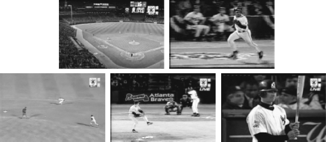
Figure 4.34 An example of typical semantics for baseball games (overview, runner, defending, pitching, batter) [49]. Source: H. Shih, and C. Huang (2003) “A Semantic Network Modeling for Understanding Baseball Video”, in Proc. ICASSP.

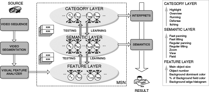
Figure 4.35 Video understanding framework proposed in [49]. Source: H. Shih, and C. Huang (2005) “MSN: Statistical Understanding of Broadcasted Baseball Video Using Multi-level Semantic Network”, IEEE Trans. Broadcasting.