CHAPTER 3
3D PROGRAMMING CONCEPTS
In this chapter we will discuss how objects are described in their three dimensions in different 3D coordinate systems, as well as how we convert them for use in the 2D coordinate system of a computer display. There is some math involved here, but don’t worry—I’ll do the heavy lifting.
We’ll also cover the stages and some of the components of the rendering pipeline—a conceptual way of thinking of the steps involved in converting an abstract mathematical model of an object into a beautiful on-screen picture.
3D CONCEPTS
In the real world, we perceive objects to have measurements in three directions, or dimensions. Typically we say they have height, width, and depth. When we want to represent an object on a computer screen, we need to account for the fact that the person viewing the object is limited to perceiving only two actual dimensions: height, from the top to the bottom of the screen, and width, across the screen from left to right.
Note
Remember that we will be using the Torque 3D engine to do most of the rendering work involved in creating our game with this book. However, a good understanding of the technology described in this section will help guide you in your decision making later on when you will be designing and building your own models or writing code to manipulate those models in real time.
Therefore, it’s necessary to simulate the third dimension, depth, “into” the screen. This on-screen three-dimensional (3D) simulation of a real (or imagined) object is called a 3D model. In order to make the model more visually realistic, we add visual characteristics, such as shading, shadows, and textures. The entire process of calculating the appearance of the 3D model—converting it to an entity that can be drawn on a two-dimensional (2D) screen and then actually displaying the resulting image—is called rendering.
Coordinate Systems
When we refer to the dimensional measurement of an object, we use number groups called coordinates to mark each vertex (corner) of the object. We commonly use the variable names X, Y, and Z to represent each of the three dimensions in each coordinate group, or triplet. There are different ways to organize the meaning of the coordinates, known as coordinate systems.
We have to decide which of our variables will represent which dimension—height, width, or depth—and in what order we intend to reference them. Then we need to decide where the zero point is for these dimensions and what it means in relation to our object. Once we have done all that, we will have defined our coordinate system.
When we think about 3D objects, each of the directions is represented by an axis, the infinitely long line of a dimension that passes through the zero point. Width or left-right is usually the X-axis, height or up-down is usually the Y-axis, and depth or near-far is usually the Z-axis. Using these constructs, we have ourselves a nice tidy little XYZ-axis system, as shown in Figure 3.1.

Now, when we consider a single object in isolation, the 3D space it occupies is called object space. The point in object space where X, Y, and Z are all 0 is normally the geometric center of an object. The geometric center of an object is usually inside the object. If positive X values are to the right, positive Y values are up, and positive Z values are away from you, then as you can see in Figure 3.2, the coordinate system is called left-handed.
Figure 3.2
Left-handed coordinate system with vertical Y-axis.
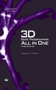
The Torque 3D engine uses a slightly different coordinate system, a right-handed one. In this system, with Y and Z oriented the same as we saw in the left-handed system, X is positive in the opposite direction. In what some people call Computer Graphics Aerobics, we can use the thumb, index finger, and middle finger of our hands to easily figure out the handedness of the system we are using (see Figure 3.3). Just remember that using this technique, the thumb is always the Y-axis, the index finger is the Z-axis, and the middle finger is the X-axis.
Figure 3.3
Right-handed coordinate system with vertical Y-axis.

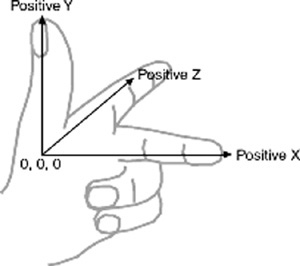
With Torque 3D, we also orient the system in a slightly different way: the Z-axis is up-down, the X-axis is somewhat left-right, and the Y-axis is somewhat near-far (see Figure 3.4). Actually, somewhat means that we specify left and right in terms of looking down on a map from above, with north at the top of the map. Right and left (positive and negative X) are east and west, respectively, and it follows that positive Y refers to north and negative Y refers to south. Don’t forget that positive Z would be up, and negative Z would be down. This is a right-handed system that orients the axes to align with the way we look at the world using a map from above. By specifying that the zero point for all three axes is a specific location on the map, and by using the coordinate system with the orientation just described, we have defined our world space.
Figure 3.4
Right-handed coordinate system with vertical Z-axis depicting world space.
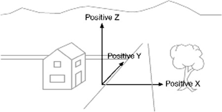
Now that we have a coordinate system, we can specify any location on an object or in a world using a coordinate triplet, such as (5, −3, −2) (see Figure 3.5). By convention, this would be interpreted as X=5, Y=−3, Z=− 2. A 3D triplet is always specified in XYZ format.
Figure 3.5
A point specified using an XYZ coordinate triplet.
Take another peek at Figure 3.5. Notice anything? That’s right—the Y-axis is vertical with the positive values above the 0, and the Z-axis positive side is toward us. It is still a right-handed coordinate system. The right-handed system with Y-up orientation is often used for modeling objects in isolation, and of course we call it object space, as described earlier. We are going to be working with this orientation and coordinate system for the next little while.
3D Models
I previously briefly touched on the idea that we can simulate, or model, any object by defining its shape in terms of its significant vertices (plural for vertex). Let’s take a closer look, by starting with a simple 3D shape, or primitive—the cube—as depicted in Figure 3.6.
Figure 3.6
Simple cube shown in a standard XYZ-axis chart.
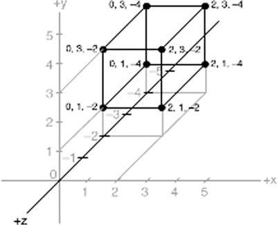
The cube’s dimensions are two units wide by two units deep by two units high, or 2 × 2 × 2. In this drawing, shown in object space, the geometric center is offset to a position outside the cube. I’ve done this in order to make it clearer what is happening in the drawing, despite my statement earlier that geometric centers are usually located inside an object. There are times when exceptions are not only possible but necessary—as in this case.
Examining the drawing, we can see the object’s shape and its dimensions quite clearly. The lower-left-front corner of the cube is located at the position where X=0, Y=1, and Z=−2. As an exercise, take some time to locate all of the other vertices (corners) of the cube, and note their coordinates.
If you haven’t already noticed on your own, there is more information in the drawing than actually needed. Can you see how we can plot the coordinates by using the guidelines to find the positions on the axes of the vertices? But we can also see the actual coordinates of the vertices drawn right in the chart. We don’t need to do both. The axis lines with their index tick marks and values really clutter up the drawing, so it has become somewhat accepted in computer graphics to not bother with these indices. Instead, we try to use the minimum amount of information necessary to completely depict the object.
We only really need to state whether the object is in object space or world space and indicate the raw coordinates of each vertex. We should also connect the vertices with lines that indicate the edges.
If you take a look at Figure 3.7 you will see how easy it is to extract the sense of the shape, compared to the drawing in Figure 3.6. We specify which space definition we are using by the small XYZ-axis notation. The color code indicates the axis name, and the axis lines are drawn only for the positive directions. Different modeling tools use different color codes, but in this book dark yellow (shown as light gray) is the X-axis, dark cyan (medium gray) is the Y-axis, and dark magenta (dark gray) is the Z-axis. It is also common practice to place the XYZ-axis key at the geometric center of the model.
Figure 3.7
Simple cube with reduced XYZ-axis key.
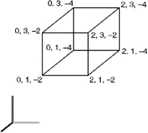
Figure 3.8 shows our cube with the geometric center placed where it reasonably belongs when dealing with an object in object space.
Now look at Figure 3.9. It is obviously somewhat more complex than our simple cube, but you are now armed with everything that you need to know to understand it. It is a screenshot of a four-view drawing from the popular shareware modeling tool MilkShape 3D, in which a 3D model of a soccer ball was created.
Figure 3.8
Simple cube with axis key at geometric center.

Figure 3.9
Screenshot of sphere model.
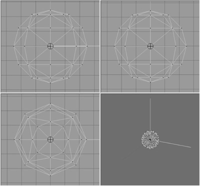
In the figure, the vertices are marked with red dots (which show as black in the picture), and the edges are marked with light gray lines. The axis keys are visible, although barely so in some views because they are obscured by the edge lines. Notice the grid lines that are used to help with aligning parts of the model. The three views with the gray background and grid lines are 2D construction views, while the fourth view, in the lower-right corner, is a 3D projection of the object. The upper-left view looks down from above, with the Y-axis in the vertical direction and the X-axis in the horizontal direction. The Z-axis in that view is not visible. The upper-right view is looking at the object from the front, with the Y-axis vertical and the Z-axis horizontal; there is no X-axis. The lower-left view shows the Z-axis vertically and the X-axis horizontally with no Y-axis. In the lower-right view, the axis key is quite evident, as its lines protrude from the model.
3D Shapes
We’ve already encountered some of the things that make up 3D models. Now it’s time to round out that knowledge.
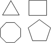
As we’ve seen, vertices define the shape of a 3D model. We connect the vertices with lines known as edges. If we connect three or more vertices with edges to create a closed figure, we’ve created a polygon. The simplest polygon is a triangle. In modern 3D accelerated graphics adapters, the hardware is designed to manipulate and display millions and millions of triangles in a second. Because of this capability in the adapters, we normally construct our models out of the simple triangle polygons instead of the more complex polygons, such as rectangles or pentagons (see Figure 3.10).
Figure 3.10
Polygons of varying complexity.
By happy coincidence, triangles are more than up to the task of modeling complex 3D shapes. Any complex polygon can be decomposed into a collection of triangles, commonly called a mesh (see Figure 3.11).
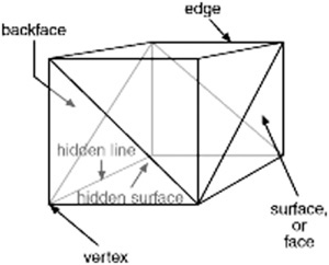
The area of the model is known as the surface. The polygonal surfaces are called facets—or at least that is the traditional name. These days, they are more commonly called faces. Sometimes a surface can only be viewed from one side, so when you are looking at it from its “invisible” side, it’s called a hidden surface or hidden face. A double-sided face can be viewed from either side. The edges of hidden surfaces are called hidden lines. With most models, there are faces on the backside of the model, facing away from us, called backfaces (see Figure 3.12). As mentioned, most of the time when we talk about faces in game development, we are talking about triangles, sometimes shortened to tris.
Figure 3.11
Polygons decomposed into triangle meshes.
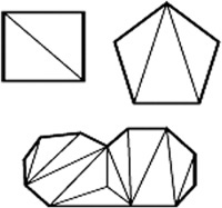
Figure 3.12
The parts of a 3D shape.
DISPLAYING 3D MODELS
After we have defined a model of a 3D object of interest, we may want to display a view of it. The models are created in object space, but to display them in the 3D world, we need to convert them to world space coordinates. This requires three conversion steps beyond the actual creation of the model in object space.
1. Convert to world space coordinates.
2. Convert to view coordinates.
3. Convert to screen coordinates.
Each of these conversions involves mathematical operations performed on the object’s vertices.
The first step is accomplished by the process called transformation. Step 2 is what we call 3D rendering. Step 3 describes what is known as 2D rendering. First we will examine what the steps do for us, before getting into the gritty details.
Transformation
This first conversion, to world space coordinates, is necessary because we have to place our object somewhere! We call this conversion transformation. We will indicate where by applying transformations to the object: a scale operation (which controls the object’s size), a rotation (which sets orientation), and a translation (which sets location).
World space transformations assume that the object starts with a transformation of (1.0,1.0,1.0) for scaling, (0,0,0) for rotation, and (0,0,0) for translation.
Every object in a 3D world can have its own 3D transformation values, often simply called transforms, that will be applied when the world is being prepared for rendering.
Tip
Other terms used for these kinds of XYZ coordinates in world space are Cartesian coordinates or rectangular coordinates.
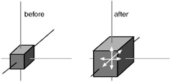
Scaling
We scale objects based upon a triplet of scale factors where 1.0 indicates a scale of 1:1.
The scale operation is written similarly to the XYZ coordinates that are used to denote the transformation, except that the scale operation shows how the size of the object has changed. Values greater than 1.0 indicate that the object will be made larger, and values less than 1.0 (but greater than 0) indicate that the object will shrink.
For example, 2.0 will double a given dimension, 0.5 will halve it, and a value of 1.0 means no change. Figure 3.13 shows a scale operation performed on a cube in object space. The original scale values are (1.0,1.0,1.0). After scaling, the cube is 1.6 times larger in all three dimensions, and the values are (1.6,1.6,1.6).
Rotation
The rotation is written in the same way that XYZ coordinates are used to denote the transformation, except that the rotation shows how much the object is rotated around each of its three axes. In this book, rotations will be specified using a triplet of degrees as the unit of measure. In other contexts, radians might be the unit of measure used. Other methods of representing rotations are used in more complex situations, but this is the way we’ll do it in this book. Figure 3.14 depicts a cube being rotated by 30 degrees around the Y-axis in its object space.
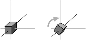
It is important to realize that the order of the rotations applied to the object matters a great deal. The convention we will use is the roll-pitch-yaw method, adopted from the aviation community. When we rotate the object, we roll it around its longitudinal (Z) axis. Then we pitch it around the lateral (X) axis. Finally, we yaw it around the vertical (Y) axis. Rotations on the object are applied in object space.
If we apply the rotation in a different order, we can end up with a very different orientation, despite having done the rotations using the same values.
Translation
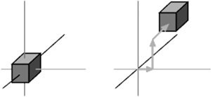
Translation is the simplest of the transformations and the last that is applied to the object when transforming from object space to world space. Figure 3.15 shows a translation operation performed on an object. Note that the vertical axis is dark gray. As I said earlier, in this book, dark gray represents the Z-axis. Try to figure out what coordinate system we are using here. I’ll tell you later in the chapter. To translate an object, we apply a vector to its position coordinates. Vectors can be specified in different ways, but the notation we will use is the same as the XYZ triplet, called a vector triplet. For Figure 3.15, the vector triplet is (3,9,7). This indicates that the object will be moved three units in the positive X direction, nine units in the positive Y direction, and seven units in the positive Z direction. Remember that this translation is applied in world space, so the X direction in this case would be eastward, and the Z direction would be down (toward the ground, so to speak). Neither the orientation nor the size of the object is changed.
Full Transformation
So now we roll all the operations together. We want to orient the cube a certain way, with a certain size, at a certain location. The transformations applied are scale (s)=1.6,1.6,1.6, followed by rotation (r)=0,30,0, and then finally translation (t)=3,9,7. Figure 3.16 shows the process.
Note
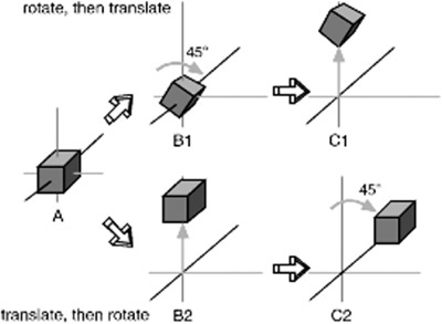
The order that we use to apply the transformations is important. In the great majority of cases, the correct order is scaling, rotation, and then translation. The reason is that different things happen depending on the order.
You will recall that objects are created in object space and then moved into world space. The object’s origin is placed at the world origin. When we rotate the object, we rotate it around the appropriate axes with the origin at (0,0,0) and then translate it to its new position.
If you translate the object first and then rotate it (which is still going to take place around (0,0,0)), the object will end up in an entirely different position, as you can see in Figure 3.17.
Figure 3.16
Fully transforming the cube.
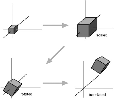
Figure 3.17
Changing the transformation order.
Rendering
Rendering is the process of converting the 3D mathematical model of an object into an on-screen 2D image. When we render an object, our primary task is to calculate the appearance of the different faces of the object, convert those faces into a 2D form, and send the result to the video card, which will then take all the steps needed to display the object on your monitor.
We will take a look at several different rendering techniques—those that are often used in video game engines or 3D video cards. There are other techniques, such as ray-casting, that aren’t in wide use in computer games (with the odd exception, of course); we won’t be covering the less-common techniques here.
In the previous sections our simple cube model had colored faces. In case you haven’t noticed (but I’m sure you did notice), we haven’t covered the issue of the faces, except briefly in passing.
A face is essentially a set of one or more contiguous coplanar adjacent triangles; that is, when taken as a whole, the triangles form a single flat surface. If you refer back to Figure 3.12, you will see that each face of the cube is made with two triangles. Of course, the faces are transparent in order to present the other parts of the cube.
Flat Shading
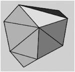
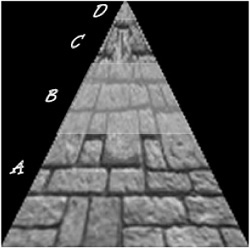
Figure 3.18 provides an example of various face configurations on an irregularly shaped object. Each face is presented with a different color (each visible as a different shade). All triangles with the label A are part of the same face; the same applies to the D triangles. The triangles labeled B and C are each single-triangle faces.
Figure 3.18
Faces on an irregularly shaped object.
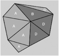
When we want to display 3D objects, we usually use some technique to apply color to the faces. The simplest method is flat shading, as used in Figure 3.18. A color or shade is applied to a face, and a different color or shade is applied to adjacent faces so that the user can tell them apart. In this case, the shades were selected with the sole criterion being the need to distinguish one face from the other.
One particular variation of flat shading is called Z-flat shading. The basic idea is that the farther a face is from the viewer, the darker or lighter the face.
Lambert Shading
Usually color and shading are applied in a manner that implies some sense of depth and lighted space. One face or collection of faces will be lighter in shade, implying that the direction they face has a light source. On the opposite side of the object, faces are shaded to imply that no light, or at least less light, reaches those faces. In between the light and dark faces, the faces are shaded with intermediate values. The result is a shaded object where the face shading provides information that imparts a sense of the object in a 3D world, enhancing the illusion. This is a form of flat shading known as lambert shading (see Figure 3.19).
Figure 3.19
Lambert-shaded object.
Gouraud Shading
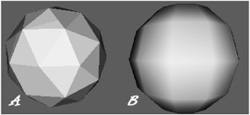
A more useful way to color or shade an object is called gouraud shading. Look at Figure 3.20. The sphere on the left (A) is flat shaded, while the sphere on the right (B) is gouraud shaded. Gouraud shading smoothes the colors by averaging the normals (the vectors that indicate which way surfaces are facing) of the vertices of a surface. The normals are used to modify the color value of all the pixels in a face. Each pixel’s color value is then modified to account for the pixel’s position within the face. Gouraud shading creates a much more natural appearance for the object, doesn’t it? Gouraud shading is commonly used in both software and hardware rendering systems.
Figure 3.20
Flat-shaded (A) and gouraud-shaded (B) spheres.
Phong Shading
Phong shading is a much more sophisticated—and computation-intensive—technique for rendering a 3D object. Like gouraud shading, it calculates color or shade values for each pixel. Unlike gouraud shading (which uses only the vertices’ normals to calculate average pixel values), phong shading computes additional normals for each pixel between vertices and then calculates the new color values. Phong shading does a remarkably better job (see Figure 3.21), but at a substantial cost.
Figure 3.21
Phong-shaded sphere.

Phong shading requires a great deal of processing for even a simple scene, which is why you don’t see phong shading used much in real-time 3D games where frame rate performance is important. However, there are games made where frame rate is not as big an issue, in which case you will often find phong shading used.
Specular Maps or Fake Phong Shading
There is a rendering technique that looks almost as good as phong shading but can allow fast frame rates. It’s called fake phong shading, or sometimes fast phong shading, or sometimes even phong approximation rendering. Whatever name it goes by, it is not phong rendering. It is useful, however, and does indeed give good performance.
Fake phong shading basically employs a bitmap, which is sometimes known as a phong map or a highlight map. The most commonly used term, and one that Torque 3D uses, is specular map. The image is nothing more than a generic template of how the faces should be illuminated (as shown in Figure 3.22).
The term “fake phong shading” has fallen out of favor in recent years. You will find the term “specular mapping” to be much more prevalent.
Texture Mapping
Texture mapping is covered in more detail in Chapters 8 and 9. For the sake of completeness, I’ll just say here that texture mapping an object is something like wallpapering a room. A 2D bitmap is “draped” over the object, to impart detail and texture upon the object, as shown in Figure 3.23.
Figure 3.22
Example of a specular map.

Figure 3.23
Texture-mapped and gouraud-shaded cube.
Texture mapping is usually combined with one of the shading techniques covered in this chapter. In many applications, and indeed, in the Torque 3D engine’s Material Editor, the basic texture map for an object is called the diffuse map.
Specular Maps
Specular maps are images that you can use to control how light reflects from an object (the object’s specularity). Rather than spend a ton of processing time calculating the reflection characteristics of an object, we can create an image that does this for us. Using specular maps is very much like fake phong shading,
Shaders
When the word is used alone, shaders refers to shader programs that are sent to the video hardware by the software graphics engine. These programs tell the video card in great detail how to manipulate vertices or pixels depending on the kind of shader used.
Traditionally, programmers have had limited control over what happens to vertices and pixels in hardware, but the introduction of shaders allowed them to take complete control.
Vertex shaders, being easier to implement, were first out of the starting blocks. The shader program on the video card manipulates vertex data values on a 3D plane via mathematical operations on an object’s vertices. The operations affect color, texture coordinates, elevation-based fog density, point size, and spatial orientation.
Pixel shaders are the conceptual siblings of vertex shaders, but they operate on each discrete viewable pixel. Pixel shaders are small programs that tell the video card how to manipulate pixel values. They rely on data from vertex shaders (either the engine-specific custom shader or the default video card shader function) to provide at least triangle, light, and view normals.
Shaders are used in addition to other rendering operations, such as texture and normal mapping.
Bump Mapping
Bump mapping is similar to texture mapping. Where texture maps add detail to a shape, bump maps enhance the shape detail. Each pixel of the bump map contains information that describes aspects of the physical shape of the object at the corresponding point, and we use a more expansive word to describe this—the texel. The name texel derives from texture pixel.
Bump mapping gives the illusion of the presence of bumps, holes, carving, scales, and other small surface irregularities. If you think of a brick wall, a texture map will provide the shape, color, and approximate roughness of the bricks. The bump map will supply a detailed sense of the roughness of the brick, the mortar, and other details. Thus bump mapping enhances the close-in sense of the object, while texture mapping enhances the sense of the object from farther away.
Bump mapping is used in conjunction with most of the other rendering techniques.
Environment Mapping
Environment mapping is similar to texture mapping, except that it is used to represent effects where environmental features are reflected in the surfaces of an object. Things like chrome bumpers on cars, windows, and other shiny object surfaces are prime candidates for environment mapping. The image in an environment map is normally a picture of what you want to be reflected in the shiny object.
Mipmapping
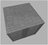
Mipmapping is a way of reducing the amount of computation needed to accurately texture-map an image onto a polygon. It’s a rendering technique that tweaks the visual appearance of an object. It does this by using several different textures for the texture-mapping operations on an object. At least two, but usually four, textures of progressively lower resolution are assigned to any given surface, as shown in Figure 3.24. The video card or graphics engine extracts pixels from each texture depending on the distance and orientation of the surface compared to the view screen.
Figure 3.24
Mipmap textures for a stone surface.
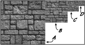
In the case of a flat surface that recedes away from the viewer into the distance, for the nearer parts of the surface, pixels from the high-resolution texture are used (see Figure 3.25). For the middle distances, pixels from the medium-resolution textures are used. Finally, for the faraway parts of the surface, pixels from the low-resolution texture are used.
Figure 3.25
Mipmap textures in perspective view.
Anti-aliasing is a software technique used in graphics display systems to make curved and diagonal lines appear to be continuous and smooth. On computer monitors the pixels themselves aren’t curved, but collectively they combine together to represent curves. Using pixels within polygon shapes to simulate curves causes the edges of objects to appear jagged. Anti-aliasing, the technique for smoothing out these jaggies, or aliasing, usually takes the form of inserting intermediate-colored pixels along the edges of the curve. The funny thing is, with textual displays this has the paradoxical effect of making text blurrier yet more readable. Go figure!
Normal Mapping
Normal mapping is a further enhancement of bump mapping. With normal mapping what we are doing, in essence, is transferring detail from a very high poly model to a low poly model using a bitmap gradient. This allows us to provide an astonishing sense of detail with very fast rendering speeds.
The basic procedure is to first create a very high polygon model of an object. Now, when I say very high, I mean just that: four or five million polygons. Yeah, 5,000,000—that high. We then make a rendered lighting pass on that object in our modeling tool and “bake” (preserve) the normals shading of the object in a bitmap very similar to the UV-mapped texture bitmap for the object. Because what we are preserving is basically a graphical representation of the normals of all of the polygons in the high poly model, the data we save is called the normal map.
We then create a low poly (in the 2,000-polygon range, give or take 500 or 1,000 polygons) model and apply the normal map to the new model. The pixel values in the normal map are used to assign brightness values to the pixels of the texture map, with almost photorealistic results at times.
Parallax Mapping
Upping the ante even further, parallax mapping is yet another evolutionary step beyond bump mapping.
With parallax mapping, we can create the illusion of holes and protrusions in flat surfaces, without adding polygons. A parallax map image is pretty well identical to a bump map, but it is used in rendering in a much more dramatic way.
Try this experiment. Set a drinking glass or cup on a table, and stand above it. Look straight down at the glass. You will obviously see the circular shape of the glass—in fact, you will probably see a series of concentric rings: the inside and outside of the opening rim, the inside and outside of the base, and so on. And in the background is the surface of the table. Now move your head to one side, while keeping your eyes on the glass. The shapes all change, even though the glass hasn’t moved. The background is still the table. Eventually, as you move your head further from the glass, the table stops being the background, starting at the top of the glass. The edge of the table “moves” down the glass toward the base. You can hasten this effect by moving your head toward the plane of the table.
Imagine now that those concentric rings that you started with were simply pixels on a bitmap, but whose values indicate a distance from the plane of a polygon (the table). Parallax-mapping software calculates where those pixels would be rendered as you move your head sideways, re-creating the changing appearance—in a 3D manner—of the glass. And yet there are no extra polygons involved! This is a simulation of the parallax effect—the apparent change of position of an object in space when viewed from a different location, even though the object hasn’t moved. The apparent change becomes visible only when the object is viewed against a static background. In the case of the little experiment I told you to do (you did do it, right?), the table is the static background.
Now when you move your head closer to the table, off to one side, or you move your head far enough away from the glass, eventually you will see that the glass really does protrude up from the table. With parallax mapping and a rendered glass, if you do the same thing, you will see the pixels of the rendered glass get squashed together and never leave the bounds of the polygon on which they are mapped. Because they can’t—they are part of the polygon! But this effect is really only visible in extreme situations that usually aren’t noticeable when you are engaged in mortal combat with a room full of electro-ninjas.
The effect is most satisfying when the parallax-mapped objects are crossing the viewer’s field of view, like when your character is walking past a series of large bullet holes or craters in a wall. Whole factories filled with pipes and machinery and valves and stuff can be rendered this way, with very little or no actual polygon budget penalties. In fact, large buckets of polygon budget can be recovered using this technique! And those polygons that were once used to create a maze of pipes and cables can now be better put to use in populating the scene with more nasty electro-ninjas.
Scene Graphs
In addition to knowing how to construct and render 3D objects, 3D engines need to know how the objects are laid out in the virtual world and how to keep track of changes in the status of the models, their orientation, and other dynamic information. This is done using a mechanism called a scene graph, a specialized form of a directed graph. The scene graph maintains information about all entities in the virtual world in structures called nodes. The 3D engine traverses this graph, examining each node one at a time to determine how to render each entity in the world. Figure 3.26 shows a simple seaside scene with its scene graph. The nodes marked by ovals are group nodes, which contain information about themselves and point to other nodes. The nodes that use rectangles are leaf nodes. These nodes contain only information about themselves.
Figure 3.26
Simple scene graph.
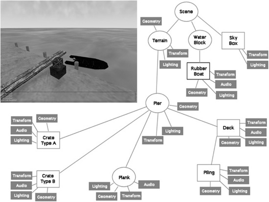
Note that in the seaside scene graph, not all of the nodes contain all of the information that the other nodes have about themselves.
Many of the entities in a scene don’t even need to be rendered. In a scene graph, a node can be anything. The most common entity types are 3D shapes, sounds, lights (or lighting information), fog and other environmental effects, viewpoints, and event triggers.
When it comes time to render the scene, the Torque 3D engine will “walk” through the nodes in the tree of the scene graph, applying whatever functions to the node that are specified. It then uses the node pointers to move on to the next node to be rendered.
3D Audio
Audio and sound effects are used to heighten the sense of realism in a game. There are times when the illusion is greatly enhanced by using position information when generating the sound effects. A straightforward example would be the sound generated by a nearby gunshot. By calculating the amplitude—based on how far away the shot occurred—and the direction, the game software can present the sound to a computer’s speakers in a way that gives the player a strong sense of where the shot occurred. This effect is even better if the player is wearing audio headphones. The player then has a good sense of the nature of any nearby threat and can deal with it accordingly—usually by massive application of return fire.
The source location of a game sound is tracked and managed in the same way as any other 3D entity via the scene graph.
Once the game engine has decided that the sound has been triggered, it then converts the location and distance information of the sound into a stereo “image” of the sound, with appropriate volume and balance for either the right or left stereo channel. The methods used to perform these calculations are much the same as those used for 3D object rendering.
Audio has an additional set of complications—things like fade and drop-off or cutoff.
3D PROGRAMMING
With the Torque 3D engine, most of the really grubby low-level programming is done for you. Instead of writing program code to construct a 3D object, you use a modeling tool (which we cover in later chapters) to create your object and a few lines of script code to insert the object in a scene. You don’t even need to worry about where in the scene graph the object should be inserted—Torque handles that as well, through the use of information contained in the data blocks that you define for objects.
Even functions like moving objects around in the world are handled for us by Torque, simply by defining the object to be of a certain class and then inserting the object appropriately.
The kinds of objects we will normally be using are called shapes. In general, shapes in Torque are considered to be dynamic objects that can move or otherwise be manipulated by the engine at run time.
There are many shape classes. Some are fairly specific, like vehicles, players, weapons, and projectiles. Some are more general-purpose classes, like items and static shapes. Many of the classes know how their objects should respond to game stimuli and are able to respond in the game with motion or some other behavior inherent to the object’s class definition.
Usually, you will let the game engine worry about the low-level mechanics of moving your 3D objects around the game world. However, there will probably be times while creating a game that you are going to want to cause objects to move in some nonstandard way—some method not defined by the class definition of the object. With Torque, this is easy to do!
Programmed Translation
When an object in 3D world space moves, it is translating its position in a manner similar to that shown earlier in the discussion about transformations.
You don’t, however, absolutely need to use the built-in classes to manipulate shapes in your game world. For example, you can write code to load in an Interior (a class of objects used for structures like buildings) or an Item (a class of objects used for smaller mobile and static items in a game world, like signs, boxes, and powerups). You can then move that object around the world any way you like.
Tip
When we move our character around within a 3D world, we often call that navigation. Navigation involves not only moving your character, but also the ability to find your way around, using aids like mini-maps, compasses, waypoints, and so on.
So don’t assume that there’s a boat or airplane somehow involved, just because you see the word “navigation” in a discussion about a computer game.
You can also write code to monitor the location of dynamic shapes that are moving around in the world, detect when they reach a certain location, and then arbitrarily jump, or teleport, those objects to some other location.
Simple Direct Movement
What we are going to do is select an object in a 3D scene in Torque using the World Editor and then move it from one location to another using some script instructions entered directly into the game console. The first step is to identify the object.
1. Run the Torque 3D tools demo by launching the Torque 3D Toolbox, then locate the FPS Example on the left side, and click the Play Game button.
2. When the promo page appears, click on the Continue Using Demo button.
3. When the main menu appears, click the Play button at the top.
4. On the next screen (Choose Level), click on the left-most image (Blank Room).
5. Click the Go! button.
Tip
You should make sure you remember steps 1 to 5 in the “Simple Direct Movement” section. These steps describe how to launch a mission in the Torque 3D Tools Demo. At later points in the book when you see that I’ve written “launch the Demo and open the such-and-such mission” somewhere in a procedure, it’s these five basic steps that I intend for you to follow. You just need to choose the appropriate mission. Yeah, I know. I’m lazy.
Reminder!
In this chapter, we are using the FPS Example for our game. This means, that the game folder can be found at 3D3EDEMOExamplesFPS Examplegame. All of the path references you will see in the procedures and discussions are relative to this game folder. So for example, when I tell you to put something in the scripts folder, then I am referring to 3D3EDEMOExamplesFPS Examplegamescripts. Get used to this concept of thinking of the game folder as the root folder within which all of your game development work is done.
6. After you’ve spawned into the game, press the F11 function key. This will load up the World Editor.
7. While in the World Editor, press the S key to move backward until you see a green octahedron (eight-sided translucent solid shape) in front of you (see Figure 3.27).
It should only take about a second’s worth of moving backward before you see the octahedron, and it should look roughly the same size as the one in Figure 3.27. If you accidentally moved the mouse before entering the World Editor and pressing the S key, then click-and-hold the right mouse button, while moving the mouse left or right until you see the green octahedron.
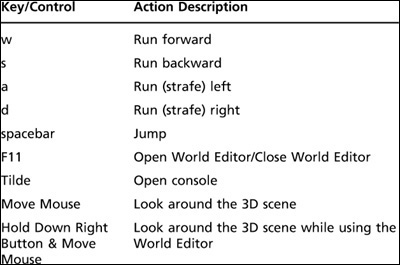
When you are not in the World Editor, you only need to move the mouse to look around. When you are in the World Editor, you need to be able to use the mouse movements to control the selection cursor. Therefore, in order to be able to look around, you hold the right mouse button down and move the mouse to look around. The navigation keys, as shown in Table 3.1, do not change between using and not using the World Editor.
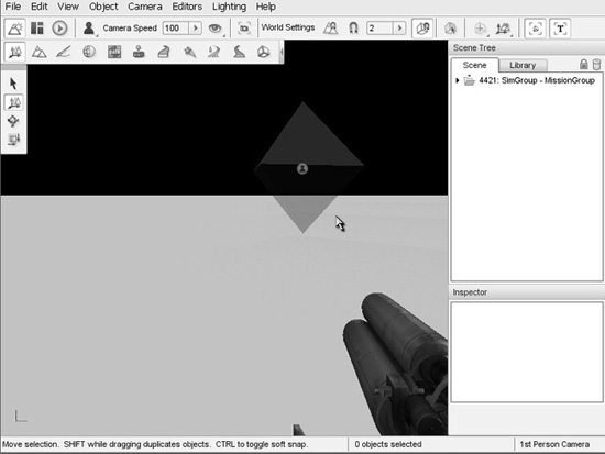
Table 3.1 Torque 3D Tools Demo Movement and Action Keys
If you still don’t see the octahedron, then stop waving the mouse around, and press the S key briefly a couple of times until it comes into view, and double-check to make sure you are indeed in the World Editor when you do this.
8. Now move your cursor to hover over top of the octahedron. Notice the white telltales appear, eight of them, giving the rough outline of the corners of a box that would enclose the octahedron. These telltales inform you that if you were to click the right mouse button right now, you would be selecting the object that the telltales highlight.
9. Press the mouse button to click on and select the octahedron while the telltales are highlighting it. You will see three colored lines appear, emanating from the center of the octahedron, as depicted in Figure 3.28 (although not in color). These lines indicate the axes of the octahedron object. The red line indicates the direction of the positive X-axis, the blue lines point up the positive Z-axis, and the green line points along the positive Y-axis.
Figure 3.28
Finding the SpawnSphere octahedron’s instance ID.
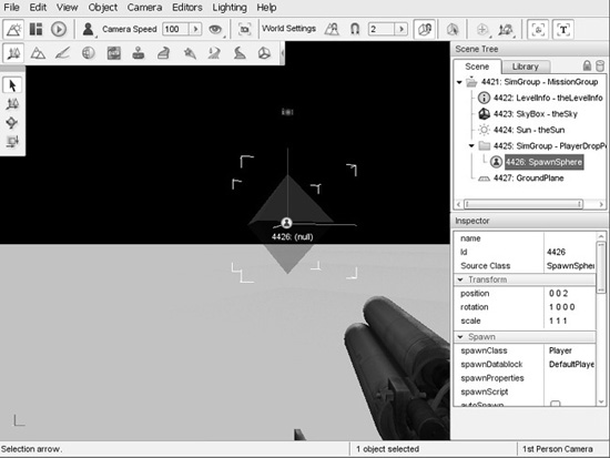
Also notice that when you clicked on the octahedron, the tree view in the Scene panel on the right expanded to show the location of the octahedron in the tree view of the scene graph. It says that it is a spawn sphere. To actually see the sphere in the 3D world (if you don’t already), press the S key to back up some more. Eventually you will see the spawn sphere.
The octahedron is the marker that specifies the actual precise location of this spawn sphere. Every spawn sphere will have a marker just like this at its center. The volume enclosed by the spawn sphere is the possible places where, when this spawn sphere is used to spawn in a character, like your character just did, to place the character in the 3D world. A sphere is used so that Torque 3D can randomly place the character in the scene with less predictability. This is a handy feature that can be used to minimize the hazards of spawn camping. The bigger the sphere, the harder it will be for a spawn camper to predict where your character will appear.
10. On the left side of the spawn sphere entry in the Scene panel’s tree view, note the green circle with what appears to be a person’s silhouette inside, that indicates that this is a spawn sphere (in addition to the actual name on the right). To the right of the icon is a number. Take note of the number that is between the icon and the word “SpawnSphere”; this is the octahedron’s instance ID. See Figure 3.28 for help, if necessary. From the tree view I get the object ID 4426, and if you look in the 3D window, just below and slightly to the left of the SpawnSphere icon at the center of the octahedron is the same Id number. You might have a different number, so write your number down or memorize it or something. Also in the 3D view, notice the word “(null)” to the right of the number. This is where the name of the spawn sphere would appear, if we had given it a name.
11. After noting the SpawnSphere’s number, move your attention to the lower-right panel, labeled “Inspector,” where the properties of the spawn sphere are located. Scroll this panel down until you come to a section called “Dynamic Fields.” In here you will find a property called “locked.” To the right of the property is a little circle with a white minus sign in it; click it, and the locked property will vanish. The SpawnSphere is now in a state where we can abuse it.
12. Press the Tilde (“~”) key, and the console will pop open. The console interface allows us to directly type in program code and get immediate results.
13. In the console window, type echo(nnnn.getTransform() ); (where nnnn is the object ID of the SpawnSphere we obtained earlier) and then press the Enter key. Don’t forget to include the semicolon at the end of the line before you press the Enter key.
You should get a result like 0 0 2 1 0 0 0, which is the transform of the Spawn-Sphere. The first three numbers are the XYZ coordinates of the geometric center of the structure. The next three are the axis normals. The final value indicates how much rotation is applied around the rotation axes. We’ll look at rotation in more detail a little later. Here, the rotation amount (which is 0) is applied to only the X-axis.
Tip
You should note that when you read the rotation angle of an object in the World Editor Inspector, the value for the rotation is given in degrees. However, when you run the getTransform method for an object, the rotation value is returned in radians. To convert between the two, 1 radian equals 57.2957795 degrees, and 1 degree equals 0.017453293 radians.
14. In the console window, type nnnn.setTransform(“0 0 0 1 0 0 0”); (where nnnn is object ID of the SpawnSphere we obtained earlier) and then press the Enter key. Notice that the console is translucent, which helps to observe the action in the 3D view.
15. Press the Tilde key to remove the console window, and take a look. You will notice that the octahedron has moved—SpawnSphere moves along with it.
16. Take the next several minutes to experiment with different transforms. Try rotating the structure around different axes or several axes at the same time.
17. When you are done, press the Tilde key to exit the console window, press Escape to exit the World Editor, and then press Escape again and then click the Yes button in the Exit from this mission dialog to exit the game.
Tip
In the little exercise in the “Simple Direct Movement” section, you saw a command that looked like this: echo(4426.getTransform() );. The number 4426 is an object ID, and the getTransform() part is what is called a method of that object. A method is a function that belongs to a specific object class. We’ll cover these topics in more detail in a later chapter.
Programmed Movement
Now we are going to explore how we can move things in the 3D world using program code. We are going to use the StaticShape class to create an object based on a model of a stylized heart, insert the object in the game world, and then start it slowly moving across the terrain—all using TorqueScript.
Okay, now—so on to the program. Using Torsion, type the following code module into a new file, and save the file as scriptsmoveshape.cs.
// ========================================================================
// moveshape.cs
//
// This module contains a function for moving a specified shape.
// ========================================================================

function MoveShape(%shape, %dist)
// ----------------------------------------------------
//       moves the %shape by %dist amount
// ----------------------------------------------------
{
  echo ("MoveShape: shape id: " , %shape);
  echo ("MoveShape: distance: " , %dist);
  %xfrm = %shape.getTransform();
  %lx = getword(%xfrm,0); // get the current transform values
  %ly = getword(%xfrm,1);
  %lz = getword(%xfrm,2);
  %ly += %dist;          // adjust the x axis position
  %shape.setTransform(%lx SPC %ly SPC %lz SPC "0 0 1 0");
  echo ("MoveShape: done.");
}
In this module there is one function that does all of the work. The function Move-Shape accepts a shape handle (or instance ID number) and a distance as arguments. It then uses these to move whatever shape the handle points to.
First, there are a couple of echo statements that print, out to the console, the shape’s handle and then the distance it will be moved.
Second, the code gets the current position of the shape using the %shape.getTransform method of the Item class.
Next, the program employs the getword function to extract the parts of the transform string that are of interest and store them in local variables. We do this because, for this particular program, we want to move the shape along the Y-axis. Therefore, we strip out all three axes and increment the Y value by the distance that the object should move. Then we prepend all three axis values to a dummy rotation and set the item’s transform to be this new string value. This last bit is done with the %shape.setTransform statement.
Finally, another echo statement hurls out to the console the basic bit of information that the module is done.
This MoveShape function acts something like a wrapper folded around the other statements. Obviously, it saves us having to type the same set of statements over and over to move different shapes different amounts at different times.
To use the program, follow these steps:
1. Make sure you’ve saved the file as scriptsmoveshape.cs.
2. Run the demo, and enter the Blank Room mission again.
3. Open the console and type in the following, making sure you press Enter after the semicolon:
exec("scripts/moveshape.cs");
If all goes well, you will see no error messages. This means that the Torque 3D engine has compiled your program and then loaded it into memory. The function you defined is now in memory, waiting with barely suppressed anticipation for your next instruction.
Tip
About those slashes... I just want to re-emphasize that when you see the filenames and paths written out, the backslash (“”) is used, and when you type in those same paths in the console window, the forward slash (“/”) is used. This is not a mistake. Torque is a cross-platform program that is available for Macintosh and Linux as well as Windows. It’s only on Windows-based systems that backslashes are used—everyone else uses forward slashes.
Therefore, the backslashes for Windows-based paths are the exception here. Just thought I’d remind you again, in case it’s not burned into your brain yet!
4. Next, make sure that the SpawnSphere object in the scene is unlocked. Whip on back to the “Simple Direct Movement” section to refresh your memory about unlocking shapes in a scene, if necessary. You will also need to obtain the SpawnSphere’s instance ID—again, the “Simple Direct Movement” section covers this.
You should be familiar with opening and closing the console window by now, so I won’t bother explaining that part in the instruction sequences anymore.
5. Type the following into the console window:
$ss=nnnn;
where nnnn is the instance ID number of the SpawnSphere. This will save that ID in the global variable $ss so that you don’t have to remember the number yourself. Note that the variable will be saved only as long as the engine is running. Once you quit Torque, the value and the variable are lost.
6. Type the following into the console window:
MoveShape($ss,50);
7. Close the console window. You should see that the sphere has moved directly away from its original location toward the “north” (positive Y).
Go ahead and experiment with the program. Try moving the SpawnSphere through several axes at once, or try changing the distance.
Programmed Rotation
As you’ve probably figured out already, we can rotate an object programmatically (or directly, for that matter) using the same setTransform method that we used to translate an object.
Type the following program, and save it as scripts urnshape.cs.
// ========================================================================
// turnshape.cs
//
// This module contains a function for turning a specified shape.
// ========================================================================

function TurnShape(%shape, %angle)
// ----------------------------------------------------
//     turns the %shape by %angle amount.
// ----------------------------------------------------
{
  echo ("TurnShape: shape id: ", %shape);
  echo ("TurnShape: angle: ", %angle);
  %xfrm = %shape.getTransform();
  echo ("TurnShape: old transform: " , %xfrm);
  %lx = getword(%xfrm,0); // first, get the current transform values
  %ly = getword(%xfrm,1);
  %lz = getword(%xfrm,2);
  %rx = getword(%xfrm,3);
  %ry = getword(%xfrm,4);
  %rz = getword(%xfrm,5);
  %angle += 1.0;         // increment the angle (ie. rotate by one degree)
  %rd = %angle;          // Set the rotation angle
  %xfrm = %lx SPC %ly SPC %lz SPC %rx SPC %ry SPC %rz SPC %rd;
  %shape.setTransform(xfrm);
  echo ("TurnShape: new transform: " , %xfrm);

  echo ("TurnShape: done.");
}
The program is quite similar to the moveshape.cs program that you were just working with. You can load and run the program in exactly the same way that you did with the moveShape module, except that you want to use TurnShape instead of MoveShape.
Note
When entering fractional values into arguments in the console when calling a function, you need to include the leading zero. For example, type 0.5—not .5.
I made two other changes: I added a couple of echo statements so that you can compare what the transform’s rotation angle value looks like after calling getTransform (when it’s in radians) to what it looks like when you call setTransform (when it requires the angle in degrees); and instead of assembling the new transform in the argument list of the call to setTransform, I stuff the new transform back into the %xfm local variable, which I then passed to setTransform. I did this so that I could also use the %xfrm variable in the ensuing echo statement. Like I’ve said before, good programmers are lazy strive for efficiency!
Things of interest to explore are the variables %rx, %ry, %rz, and %rd in the Turn-Shape function. Try making changes to each of these, and then observe the effects your changes have on the item.
Programmed Scaling
We can also quite easily change the scale of an object using program code.
Type the following program, and save it as scriptssizeshape.cs.
// ========================================================================
// sizeshape.cs
//
// This module contains a function for scaling a specified shape.
// ========================================================================

function SizeShape(%shape, %scale)
// ----------------------------------------------------
//     resizes the %shape by %scale amount
// ----------------------------------------------------
{
   echo ("SizeShape: shape id: ", %shape);
   echo ("SizeShape: angle: ", %scale);
   %shape.setScale(%scale SPC %scale SPC %scale);
   echo ("SizeShape: done.");
}
Ha! You thought there would be a ton o’ typing in store, didn’t you? Well, the program is obviously similar to the moveshape.cs and turnshape.cs programs, sort of. Except for all of the missing bits, that is. You can load and run this program in exactly the same way, except that you want to use SizeShape instead of MoveShape or TurnShape.
Why bother to write all this code to replace what is essentially a single line statement anyway (if you ignore the echo statements)? For the practice, of course!
You’ll note that we don’t call the object’s %shape.getScale function (there is one), because in this case, we don’t need to. Also notice that the three arguments to our call to %shape.setScale all use the same value. This is to make sure the object scales equally in all dimensions. Try making changes to each of these, and then observe the effects your changes have on the item.
Another exercise would be to modify the SizeShape function to accept a different parameter for each dimension (X, Y, or Z) so that you can change all three to different scales at the same time.
Programmed Animation
You can animate objects by stringing together a bunch of translation, rotation, and scale operations in a continuous loop. Like the transformations, most of the animation in Torque can be left up to an object’s class methods to perform. However, you can create your own ad hoc animations quite easily by using the schedule function.
Type the following program, and save it as scriptsanimshape.cs.
// ========================================================================
// animshape.cs
//
// This module contains functions for animating a shape using
// a recurring scheduled function call.
// ========================================================================

function AnimShape(%shape, %dist, %angle, %scale)
// ----------------------------------------------------
//   moves the %shape by %dist amount, and then
//   schedules itself to be called again in 1/5
//   of a second.
// ----------------------------------------------------
{
  echo("AnimShape: shape:", %shape, " dist:",
        %dist, " angle:", %angle, " scale:", %scale);
  if ( %shape $= "" ||
      %dist $= ""  ||
      %angle $= "" ||
      %scale $= "" )
  {
    error("AnimShape needs 4 parameters.syntax:" );
    error("AnimShape(id,moveDist,turnAng,scaleVal);"  );
    return;
  }
  %xfrm = %shape.getTransform();
  %lx = getword(%xfrm,0);   // first, get the current
  %ly = getword(%xfrm,1);            // transform values
  %lz = getword(%xfrm,2);
  %rx = getword(%xfrm,3);
  %ry = getword(%xfrm,4);
  %rz = getword(%xfrm,5);
  %lx += %dist;           // set the new x position
  %angle += 1.0;
  %rd = %angle;           // Set the rotation angle

  if ($grow)      // if the shape is growing larger
  {
   if (%scale < 5.0)   // and hasn't gotten too big
    %scale += 0.3;      // make it bigger
   else
    $grow = false; // if it's too big, then
  }                   // don't let it grow more
  else                // if it's shrinking
  {
   if (%scale > 3.0)   // and isn't too small
    %scale -= 0.3;      // then make it smaller
   else
    $grow = true;   // if it's too small,
  }                // don't let it grow smaller

 %shape.setScale(%scale SPC %scale SPC %scale);
 %shape.setTransform(%lx SPC %ly SPC %lz SPC
                       %rx SPC %ry SPC %rz SPC %rd);
 schedule(200,0,AnimShape, %shape, %dist, %angle, %scale);
}

function DoAnimTest(%shape)
{
  if (%shape $= "" && isObject(%shape))
  {
     error("DoAnimTest requires 1 parameter.");
     error("DoAnimTest syntax: DoAnimTest(shapeID);");
     return;
  }
  $grow = true;
  AnimShape(%shape, 0.2, 1, 2);
}
This module contains code from all of the three earlier modules and ties them together in a way that allows us to watch an absolutely nutso octahedron gyrate and gambol about the countryside, such as it is.
The function AnimShape accepts a shape handle as %shape, a distance step as %dist, an angle value as %angle, and a scaling value as %scale and uses these to transform the shape indicated by the %shape handle.
Before getting under way though, the function checks to make sure that it has values for all of the parameters.
First, it obtains the current position of the shape using the %shape.getTransform method of the Item class.
As with the earlier MoveShape function, the AnimShape function fetches the transform of the shape and updates one of the axis values.
Then it updates the rotation value stored as %rd.
Then it adjusts the scale value by determining if the shape is growing or shrinking. Depending on which way the size is changing, the scale is incremented, unless the scale exceeds the too large or too small limits. When a limit is exceeded, the change direction is reversed.
Next, the scale of the shape is changed to the new values using the % shape.setScale method for the shape.
Finally, the function sets the item’s transform to be the new transform values within the %shape.setTransform statement.
The DoAnimTest function accepts an object handle and verifies that it is valid, emitting an error message and exiting via the return statement if there is no valid object ID.
Then the global variable called $grow is set to true. This variable operates as a flag, and will determine whether the shape will start out by scaling up in size or not. This function then calls the AnimShape function, specifying which shape to animate by passing in the handle to the shape as the first argument and also indicating the discrete movement step distance, the discrete rotation angle, and the discrete size change value with the second, third, and fourth arguments.
To use the program, follow these steps:
1. Make sure you’ve saved the file as scriptsanimshape.cs.
2. Run the demo.
3. After spawning in, press F11, back up a little, and obtain the id number of the SpawnSphere. It probably hasn’t changed from before, but it might.
4. Bring up the console window.
5. Type in the following, and press Enter after the semicolon:
exec("scripts/animshape.cs");
If there are no errors, nothing will be printed in the console. This means that the Torque 3D engine has compiled your program and then loaded it into memory. The data block definition and the three functions are in memory, waiting to be used.
6. Now, type the following into the console, and close the console quickly afterward:
DoAnimTest($ss);
Remember that $ss is the variable that holds the instance handle of the Spawn-Sphere. You will need to assign the correct value (obtained from step 3) into this variable first—check back in the “Programmed Movement” section for a quick refresher, if necessary. You can also, if you like, type the id number directly into the function call’s argument list without using the variable.
What you should see now is the SpawnSphere start spinning and moving toward you a bit, and then away, while the octahedron marker inside it is growing and then shrinking.
Go ahead and experiment with the program. Try moving the item through several axes at once, or try changing the distance. I did not put any code in the animtest module to stop the animation. Review Chapter 2 and the preceding section in this chapter and see if you can add statements that will stop the animation when certain conditions are met.
3D Audio
Environmental sounds with a 3D component contribute greatly to the immersive aspect of a game by providing positional cues that mimic the way sounds happen in real life.
We can control 3D audio in the scene in much the same way we do 3D visual objects.
Type the following program, and save it as scriptsanimaudio.cs.
// ========================================================================
// animaudio.cs
//
// This module contains the definition of an audio emitter, which uses
// a synthetic water drop sound. It also contains functions for placing
// the test emitter in the game world and moving the emitter.
// ========================================================================

datablock SFXProfile(TestSound)
// ----------------------------------------------------
//     Definition of the audio profile
// ----------------------------------------------------
{
  filename = "art/sound/testing.ogg"; // wave file to use for the sound
  description = "AudioDefaultLooping3d"; // monophonic sound that repeats
    preload = false; // Engine will only load sound if it encounters it
                     // in the mission
};

function InsertTestEmitter()
// ----------------------------------------------------
//   Instantiates the test sound, then inserts it
//   into the game world to the right and offset somewhat
//   from the player's default spawn location.
// ----------------------------------------------------
{
  // An example function which creates a new TestSound object
  %emtr = new SFXEmitter() {
     position = "0 0 0" ;
     rotation = "1 0 0 0";
     scale = "1 1 1";
     canSaveDynamicFields = "1";
     profile = "TestSound"; // Use the profile in the datablock above
     playOnAdd = "1" ;
     isLooping = "1" ;
     isStreaming = "0" ;
     channel = "2";
     volume = "1";
     pitch = "1";
     fadeInTime = "0";
     fadeOutTime = "0" ;
     is3D = "1";
     referenceDistance = "10"   ;
     maxDistance = "50";
     coneInsideAngle = "360";
     coneOutsideAngle = "360"   ;
     coneOutsideVolume = "0";
  };
  //ensures object is removed when mission is ended
  MissionCleanup.add(%emtr);

  %emtr.setTransform("-10 0 0 0 0 1 0"); // starting location
  echo("Inserting Audio Emitter " @ %emtr);
  return %emtr;
}

function AnimSound(%snd, %dist)
// ----------------------------------------------------
//     moves the %snd by %dist amount each time
// ----------------------------------------------------
{
   %xfrm = %snd.getTransform();
   %lx = getword(%xfrm,0); // first, get the current transform values
   %ly = getword(%xfrm,1);
   %lz = getword(%xfrm,2);
   %rx = getword(%xfrm,3);
   %ry = getword(%xfrm,4);
   %rz = getword(%xfrm,5);
   %lx += %dist;            // set the new x position
   %snd.setTransform(%lx SPC %ly SPC %lz SPC %rx SPC %ry SPC %rz SPC %rd);
   schedule(200,0,AnimSound, %snd, %dist);

}

function DoAudioMoveTest()
// ----------------------------------------------------
//     a function to tie together the instantiation
//     and the movement in one easy to type function
//     call.
// ----------------------------------------------------
{
     %ms = InsertTestEmitter();
     AnimSound(%ms,1);
}
DoAudioMoveTest();   // by putting this here, we cause the test to start
                    // as soon as this module has been loaded into memory
In this program, we also have a data block that defines an audio profile. It contains the name of the ogg (sound) file that contains the sound to be played, a descriptor that tells Torque how to treat the sound, and a flag to indicate whether the engine should automatically load the sound or wait until it encounters a need for the sound. In this case, the engine will wait until it knows it needs the file.
Note
Torque supports both wave (.wav) and Ogg Vorbis (.ogg) audio file formats. If you do not include the extension part of an audio file’s name when specifying one in a data block or an audio object, Torque will automatically tack the .wav extension onto the filename and then go look for the audio file. If Torque cannot find the file using the .wav extension, it will then add the .ogg extension instead and go look for the file again.
If you do include an extension (.wav or .ogg) as part of the filename, then Torque will look for the specified filename with extension and give up if the file is not found.
The InsertTestEmitter function creates an audio object with a call to new SFXEmitter, and there are quite a few properties to be set. These properties will be explained in greater detail in Chapter 20.
A difference to note compared to the earlier modules you created is the last line, which is a call to DoAudioMoveTest. This allows us to load and run the program in one go, using the exec call. After the Torque 3D engine compiles the program, it loads it into memory and runs through the code. In our earlier program, like the AnimShape module, Torque would encounter only the data block and function definitions. Because they are definitions, they aren’t executed—they’re just loaded into memory. The last line, however, is not a definition. It is a statement that calls a function. So when Torque encounters it, Torque looks to see if it has the function resident in memory, and if so, it executes the function according to the syntax of the statement. Statements in script modules that are not part of function definitions or data block definitions are sometimes called naked statements, or more commonly, inline statements. They are “inline” because they are executed as soon as they are encountered (as if in a lineup), not saved elsewhere in memory prior to being used.
To use the program, follow these steps:
1. Make sure you’ve saved the file as scriptsanimaudio.cs.
2. Run the demo and launch the World Editor.
3. After you spawn in, just back away from the spawn sphere until you can see the sphere clearly.
4. Bring up the console window.
5. Type in the following, and press Enter after the semicolon:
exec("scripts/animaudio.cs");
You should also begin to hear the dripping “test” sound appearing to be off to the center-left side. If you wait without moving your player in any way, not even using the mouse to turn his head, you will notice the sound slowly approach you on the left, pass over to the right in front of you, and then go off into the distance to the right. Pretty cool, huh?
You’ll also notice, while in the World Editor, an icon that looks like a little speaker blasting out sound sidling from left to right. That is the construct that represents the sound emitter.
MOVING RIGHT ALONG
So, we’ve now seen how 3D objects are constructed from vertices and faces, or polygons. We explored how they fit into that virtual game world using transformations and that the transformations are applied in a particular order—scaling, rotation, and then finally translation. We also saw how different rendering techniques can be used to enhance the appearance of 3D models.
Then we learned practical ways to apply those concepts using program code written using TorqueScript and tested with the Torque 3D game engine.
In the next chapter, we will dive deeper into learning how to use TorqueScript, and how to apply it in the context of a game.