
4
Deadlock
CONTENTS
4.2 Formal Definition of Deadlock
4.3 Reasoning about Deadlock: The Resource Allocation Graph
In any concurrent system, process execution relies on the availability of a number of resources such as, for example, disk blocks, memory areas, and input–output (I/O) devices. Resources are often in scarce supply, hence they must be shared among all processes in the system, and processes compete with each other to acquire and use them.
In this chapter we will see that uncontrolled resource sharing may be very dangerous and, in particular, may prevent whole groups of processes from performing their job. Even if the probability of occurrence of this unfortunate phenomenon, known as deadlock, may be very low, it must still be dealt with adequately, especially in a real-time system.
4.1 A Simple Example
In any multiprogrammed system, many processes usually share a certain number of resources and compete for their use. The concept of resource is very broad and includes both physical resources, for example, printers, disk blocks, and memory areas, as well as logical ones, like entries in the operating system’s data structures or filesystem tables.
Some kinds of resource, such as a read-only data structure, pose no problems in this respect because many processes can access them concurrently with correct results. However, many other resources can intrinsically be used by only one process at a time. For instance, having multiple processes simultaneously using the same disk block for storage must be avoided because this would lead to incorrect results and loss of data.
To deal with this problem, most operating systems compel the processes under their control to request resources before using them and wait if those resources are currently assigned to another process, so that they are not immediately available for use. Processes must also release their resources when they no longer need them, in order to make them available to others. In this way, the operating system acts as an arbiter for what concerns resource allocation and can ensure that processes will have exclusive access to them when required.
Unless otherwise specified, in this chapter we will only be concerned with reusable resources, a term taken from historical IBM literature [33]. A reusable resource is a resource that, once a process has finished with it, is returned to the system and can be used by the same or another process again and again. In other words, the value of the resource or its functionality do not degrade with use. This is in contrast with the concept of consumable resource, for example, a message stored in a FIFO queue, that is created at a certain point and ceases to exist as soon as it is assigned to a process.
In most cases, processes need more than one resource during their lifetime in order to complete their job, and request them in succession. A process A wanting to print a file may first request a memory buffer in order to read the file contents into it and have a workspace to convert them into the printer-specific page description language. Then, it may request exclusive use of the printer and send the converted data to it. We leave out, for clarity, the possibly complex set of operations A must perform to get access to the file.
If the required amount of memory is not immediately available, it is reasonable for the process to wait until it is, instead of failing immediately because it is likely that some other process will release part of its memory in the immediate future. Likewise, the printer may be assigned to another process at the time of the request and, also in this case, it is reasonable to wait until it is released.
Sadly, this very common situation can easily lead to an anomalous condition, known as deadlock, in which a whole set of processes is blocked forever and will no longer make any progress. Not surprisingly, this problem has received a considerable amount of attention in computer science; in fact, one of the first formal definitions of deadlock was given by in 1965 by Dijkstra [23], who called it “deadly embrace.”
To illustrate how a deadlock may occur in our running example, let us consider a second process B that runs concurrently with A. It has the same goal as process A, that is, to print a file, but is has been coded in a different way. In particular, process B request the printer first, and then it tries to get the memory buffer it needs. The nature of this difference is not at all important (it may be due, for example, to the fact that A and B have been written by two different programmers unaware of each other’s work), but it is nonetheless important to realize that both approaches are meaningful and there is nothing wrong with either of them.
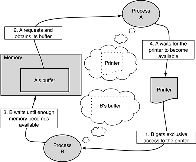
FIGURE 4.1
A simple example of deadlock involving two processes and two resources.
In this situation, the sequence of events depicted in Figure 4.1 may occur:
Process B request the printer, P. Since the printer has not been assigned to any process yet, the request is granted immediately and B continues.
Process A requests a certain amount MA of memory. If we assume that the amount of free memory at the time of the request is greater than MA, this request is granted immediately, too, and A proceeds.
Now, it is the turn of process B to request a certain amount of memory MB. If the request is sensible, but there is not enough free memory in the system at the moment, the request is not declined immediately. Instead, B is blocked until a sufficient amount of memory becomes available.
This may happen, for example, when the total amount of memory M in the system is greater than both MA and MB, but less than MA + MB, so that both requests can be satisfied on their own, but not together.
When process A requests the printer P, it finds that it has been assigned to B and that it has not been released yet. As a consequence, A is blocked, too.
At this point, both A and B will stay blocked forever because they own a resource, and are waiting for another resource that will never become available since it has been assigned to the other process involved in the deadlock.
Even in this very simple example, it is evident that a deadlock is a complex phenomenon with a few noteworthy characteristics:
It is a time-dependent issue. More precisely, the occurrence of a deadlock in a system depends on the relationship among process timings. The chain of events leading to a deadlock may be very complex, hence the probability of actually observing a deadlock during bench testing may be very low. In our example, it can easily be observed that no deadlock occurs if process A is run to completion before starting B or vice versa.
Unfortunately, this means that the code will be hard to debug, and even the insertion of a debugger or code instrumentation to better understand what is happening may perturb system timings enough to make the deadlock disappear. This is a compelling reason to address deadlock problems from a theoretical perspective, during system design, rather than while testing or debugging it.
It also depends on a few specific properties of the resources involved and on how the operating system manages them. For example, albeit this technique is not widespread in real-time operating systems, some general-purpose operating systems are indeed able to swap process images in and out of main memory with the assistance of a mass storage device. Doing this, they are able to accommodate processes whose total memory requirements exceed the available memory.
In this case, the memory request performed by B in our running example does not necessarily lead to an endless wait because the operating system can temporarily take away—or preempt—some memory from A in order to satisfy B’s request, so that both process will be eventually able to complete their execution. As a consequence, the same processes may or may not be at risk for what concerns deadlock, when they are executed by operating systems employing dissimilar memory management or, more generally, resource management techniques.
4.2 Formal Definition of Deadlock
In the most general way, a deadlock can be defined formally as a situation in which a set of processes passively waits for an event that can be triggered only by another process in the same set. More specifically, when dealing with resources, there is a deadlock when all processes in a set are waiting for some resources previously allocated to other processes in the same set. As discussed in the example of Section 4.1, a deadlock has therefore two kinds of adverse consequences:
The processes involved in the deadlock will no longer make any progress in their execution, that is, they will wait forever.
Any resource allocated to them will never be available to other processes in the system again.
Havender [33] and Coffman et al. [20] were able to formulate four conditions that are individually necessary and collectively sufficient for a deadlock to occur. These conditions are useful, first of all because they define deadlock in a way that abstracts away as much as possible from any irrelevant characteristics of the processes and resources involved.
Second, they can and have been used as the basis for a whole family of deadlock prevention algorithms because, if an appropriate policy is able to prevent (at least) one of them from ever being fulfilled in the system, then no deadlock can possibly occur by definition. The four conditions are
Mutual exclusion: Each resource can be assigned to, and used by, at most one process at a time. As a consequence, a resource can only be either free or assigned to one particular process. If any process requests a resource currently assigned to another process, it must wait.
Hold and Wait: For a deadlock to occur, the processes involved in the deadlock must have successfully obtained at least one resource in the past and have not released it yet, so that they hold those resources and then wait for additional resources.
Nonpreemption: Any resource involved in a deadlock cannot be taken away from the process it has been assigned to without its consent, that is, unless the process voluntarily releases it.
Circular wait: The processes and resources involved in a deadlock can be arranged in a circular chain, so that the first process waits for a resource assigned to the second one, the second process waits for a resource assigned to the third one, and so on up to the last process, which is waiting for a resource assigned to the first one.
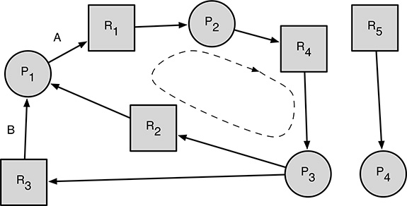
FIGURE 4.2
A simple resource allocation graph, indicating a deadlock.
4.3 Reasoning about Deadlock: The Resource Allocation Graph
The resource allocation graph is a tool introduced by Holt [39] with the twofold goal of describing in a precise, rigorous way the resource allocation state in a system at a given instant, as well as being able to reason about and detect deadlock conditions. Figure 4.2 shows an example.
In its simplest form, a resource allocation graph is a directed graph with two kinds of nodes and two kinds of arcs. The two kinds of nodes represent the processes and resources of interest, respectively. In the most common notation, used, for example, by Tanenbaum and Woodhull [85] and Silbershatz et al. [83]:
Processes are shown as circles.
Resources are shown as squares.
For instance, in Figure 4.2, P2 represents a process and R1 represents a resource. Of course, the exact geometric shape used to represent processes and resources is not at all important. As a matter of fact, in the Holt’s paper [39] the notation was exactly the opposite.
On the other hand, the two kinds of arcs express the request and ownership relations between processes and resources. In particular,
An arc directed from a process to a resource (similar to the arc labeled A in Figure 4.2, going from process P1 to resource R1) indicates that the process is waiting for the resource.
An arc directed from a resource to a process (for example, arc B in Figure 4.2, going from resource R3 to process P1) denotes that the resource is currently assigned to, or owned by, the process.
Hence, the resource allocation graph shown in Figure 4.2 represents the following situation:
Process P1 owns resources R2 and R3, and is waiting for R1.
Process P2 owns resource R1 and is waiting for resource R4.
Process P3 owns resource R4 and is waiting for two resources to become available: R2 and R3.
Process P4 owns resource R5 and is not waiting for any other resource.
It should also be noted that arcs connecting either two processes, or two resources, have got no meaning and are therefore not allowed in a resource allocation graph. More formally, the resource allocation graph must be bipartite with respect to process and resource nodes.
The same kind of data structure can also be used in an operating system to keep track of the evolving resource request and allocation state. In this case,
When a process P requests a certain resource R, the corresponding “request arc,” going from P to R, is added to the resource allocation graph.
As soon as the request is granted, the request arc is replaced by an “ownership arc,” going from R to P. This may either take place immediately or after a wait. The latter happens, for example, if R is busy at the moment. Deadlock avoidance algorithms, discussed in Section 4.6, may compel a process to wait, even if the resource it is requesting is free.
When a process P releases a resource R it has previously acquired, the ownership arc going from R to P is deleted. This arc must necessarily be present in the graph, because it must have been created when R has been granted to P.
For this kind of resource allocation graph, it has been proved that the presence of a cycle in the graph is a necessary and sufficient condition for a deadlock. It can therefore be used as a tool to check whether a certain sequence of resource requests, allocations, and releases leads to a deadlock. It is enough to keep track of them, by managing the arcs of the resource allocation graph as described earlier, and check whether or not there is a cycle in the graph after each step.
If a cycle is found, then there is a deadlock in the system, and the deadlock involves precisely the set of processes and resources belonging to the cycle. Otherwise the sequence is “safe” from this point of view. The resource allocation graph shown in Figure 4.2 models a deadlock because P1 → R1 → P2 → R4 → P3 → R2 → P1 is a cycle. Processes P1, P2, and P3, as well as resources R1, R2, and R4 are involved in the deadlock. Likewise, P1 → R1 → P2 → R4 → P3 → R3 → P1 is a cycle, too, involving the same processes as before and resources R1, R3, and R4.
As for any directed graph, also in this case arc orientation must be taken into account when assessing the presence of a cycle. Hence, referring again to Figure 4.2, P1 ← R2 ← P3 → R3 → P1 is not a cycle and does not imply the presence of any deadlock in the system.
The deadlock problem becomes more complex when there are different kinds (or classes) of resources in a system and there is, in general, more than one resource of each kind. All resources of the same kind are fungible, that is, they are interchangeable so that any of them can be used to satisfy a resource request for the class they belong to.
This is a common situation in many cases of practical interest: if we do not consider data access time optimization, disk blocks are fungible resources because, when any process requests a disk block to store some data, any free block will do. Other examples of fungible resources include memory page frames and entries in most operating system tables.
The definition of resource allocation graph can be extended to handle multiple resource instances belonging to the same class, by using one rectangle for each resource class, and representing each instance by means of a dot drawn in the corresponding rectangle. In Reference [39], this is called a general resource graph.
However, in this case, the theorem that relates cycles to deadlocks becomes weaker. It can be proved [39] that the presence of a cycle is still a necessary condition for a deadlock to take place, but it is no longer sufficient. The theorem can hence be used only to deny the presence of a deadlock, that is, to state that if there is not any cycle in an extended resource allocation graph, then there is not any deadlock in the system.
4.4 Living with Deadlock
Deadlock is a time-dependent problem, and the probability of actually encountering a deadlock during operation is often quite small with respect to other issues such as, for example, power interruptions or other software bugs. On the other hand, deadlock may also be a very complex problem to deal with, and its handling may consume a considerable amount of system resources.
It is therefore not a surprise if some operating system designers deliberately decided to completely neglect the problem, at least in some cases, and adopt a strategy sometimes called “the Ostrich algorithm” [85]. In this sense, they are trading off a small probability of being left with a (partially) deadlocked system for a general improvement of system performance.
This reasoning usually makes sense for general-purpose operating systems. For example, Bach [10] highlights the various situations in which the Unix operating system is, or (more commonly) is not, protected against deadlock. Most other operating systems derived from Unix, for example, Linux, suffer from the same problems.
On the contrary, in many cases, real-time applications cannot tolerate any latent deadlock, regardless of its probability of occurrence, for instance, due to safety concerns. Once it has been decided to actually “do something” about deadlock, the algorithms being used can be divided into three main families:
Try to prevent deadlock, by imposing some constraints during system design and implementation.
Check all resource requests made by processes as they come by and avoid deadlock by delaying resource allocation when appropriate.
Let the system possibly go into a deadlock, but then detect this situation and put into effect a recovery action.
The main trade-offs between these techniques have to do with several different areas of application development and execution, and all of them should be considered to choose the most fruitful technique for any given case. In particular, the various families differ regarding
When deadlock handling takes place. Some techniques must be applied early in system design, other ones take action at run time.
How much influence they have in the way designers and programmers develop the application.
How much and what kind of information about processes behavior they need, in order to work correctly.
The amount of run time overhead they inflict on the system.
4.5 Deadlock Prevention
The general idea behind all deadlock prevention techniques is to prevent deadlocks from occurring by making sure that (at least) one of the individually necessary conditions presented in Section 4.2 can never be satisfied in the system. In turn, this property is ensured by putting into effect and enforcing appropriate design or implementation rules, or constraints.
Since there are four necessary conditions, four different deadlock prevention strategies are possible, at least in principle. Most of the techniques to be presented in this section have been proposed by Havender [33].
The mutual exclusion condition can be attacked by allowing multiple processes to use the same resource concurrently, without waiting when the resource has been assigned to another process.
This goal cannot usually be achieved by working directly on the resource involved because the need for mutual exclusion often stems from some inescapable hardware characteristics of the resource itself. For example, there is no way to modify a CD burner and allow two processes to write on a CD concurrently.
On the contrary, an equivalent result can sometimes be obtained by interposing an additional software layer between the resource and the processes competing for it: for printers, it is common to have spoolers devoted to this purpose. In its simplest form, a spooler is a system process that has permanent ownership of a certain printer. Its role is to collect print requests from all the other processes in the system, and carry them out one at a time.
Even if the documents to be printed are still sent to the printer sequentially, in order to satisfy the printer’s mutual exclusion requirements, the spooler will indeed accept multiple, concurrent print requests because it will use another kind of media, for example, a magnetic disk, to collect and temporarily store the documents to be printed.
Hence, from the point of view of the requesting processes, resource access works “as if” the mutual exclusion constraint had been lifted, and deadlock cannot occur, at least as long as the disk space available for spooling is not so scarce to force processes to wait for disk space while they are producing their output. The latter condition may intuitively lead to other kinds of deadlock, because we are merely “shifting” the deadlock problem from one resource (the printer) to another (the spooling disk space).
Nevertheless, the main problem of spooling techniques is their limited applicability: many kinds of resource are simply not amenable to be spooled. To make a very simple example, it is totally unclear how it would be possible to spool an operating system data structure.
The hold and wait condition is actually made of two parts that can be considered separately. The wait part can be invalidated by making sure that no processes will ever wait for a resource. One particularly simple way of achieving this is to force processes to request all the resources they may possibly need during execution all together and right at the beginning of their execution.
Alternatively, processes can be constrained to release all the resources they own before requesting new ones, thus invalidating the hold part of the condition. The new set of resources being requested can include, of course, some of the old ones if they are still needed, but the process must accept a temporary loss of resource ownership anyway. If a stateful resource, like for instance a printer, is lost and then reacquired, the resource state will be lost, too.
In a general purpose system, it may be difficult, or even impossible, to know in advance what resources any given application will need during its execution. For example, the amount of memory or disk space needed by a word processor is highly dependent on what the user is doing with it and is hard to predict in advance.
Even when it is possible to agree upon a reasonable set of resources to be requested at startup, the efficiency of resource utilization will usually be low with this method, because resources are requested on the basis of potential, rather than actual necessity. As a result, resources will usually be requested a long time before they are really used. When following this approach, the word processor would immediately request a printer right when it starts—this is reasonable because it may likely need it in the future—and retain exclusive access rights to it, even if the user does not actually print anything for hours.
When considering simple real-time systems, however, the disadvantages of this method, namely, early resource allocation and low resource utilization, are no longer a limiting factor, for two reasons. First of all, low resource utilization is often not a concern in those systems. For example, allocating an analog-to-digital converter (ADC) to the process that will handle the data it produces well before it is actively used may be perfectly acceptable. This is due to the fact that the resource is somewhat hardwired to the process, and no other processes in the system would be capable of using the same device anyway even if it were available.
Second, performing on-demand resource allocation to avoid allocating resources too early entails accepting the wait part of this condition. As a consequence, processes must be prepared to wait for resources during their execution. In order to have a provably working hard real-time system, it must be possible to derive an upper bound of the waiting time, and this may be a difficult task in the case of on-demand resource allocation.
The nonpreemption condition can be attacked by making provision for a resource preemption mechanism, that is, a way of forcibly take away a resource from a process against its will. Like for the mutual exclusion condition, the difficulty of doing this heavily depends on the kind of resource to be handled. One the one hand, preempting a resource such as a processor is quite easy, and is usually done (by means of a context switch) by most operating systems.
On the other hand, preempting a print operation already in progress in favor of another one entails losing a certain amount of work (the pages printed so far) even if the print operation is later resumed at the right place, unless a patient operator is willing to put the pieces together. As awkward as it may seem today, this technique was actually used in the past: in fact, the THE operating system might preempt the printer on a page-by-page basis [26, 24].
The circular wait condition can be invalidated by imposing a total ordering on all resource classes and imposing that, by design, all processes follow that order when they request resources. In other words, an integer-valued function f (Ri) is defined on all resource classes Ri and it has a unique value for each class. Then, if a process already owns a certain resource Rj, it can request an additional resource belonging to class Rk if, and only if, f (Rk) > f (Rj).
It can easily be proved that, if all processes obey this rule, no circular wait may occur in the system [83]. The proof proceeds by reductio ad absurdum.
Assume that, although all processes followed the rule, there is indeed a circular wait in the system. Without loss of generality, let us assume that the circular wait involves processes P1, ..., Pm and resource classes R1, ..., Rm, so that process P1 owns a resource of class R1 and is waiting for a resource of class R2, process P2 owns a resource of class R2 and is waiting for a resource of class R3, ... process Pm owns a resource of class Rm and is waiting for a resource of class R1, thus closing the circular wait.
If process P1 followed the resource request rule, then it must be
because P1 is requesting a resource of class R2 after it already obtained a resource of class R1.
The same reasoning can be repeated for all processes, to derive the following set of inequalities:
Due to the transitive property of inequalities, we come to the absurd:
and are able to disprove the presence of a circular wait.
In large systems, the main issue of this method is the difficulty of actually enforcing the design rules and check whether they have been followed or not. For example, the multithreaded FreeBSD operating system kernel uses this approach and orders its internal locks to prevent deadlocks. However, even after many years of improvements, a fairly big number of “lock order reversals”—that is, situations in which locks are actually requested in the wrong order—are still present in the kernel code. In fact, a special tool called
witnesswas even specifically designed to help programmers detect them [12].
4.6 Deadlock Avoidance
Unlike deadlock prevention algorithms, discussed in Section 4.5, deadlock avoidance algorithms take action later, while the system is running, rather than during system design. As in many other cases, this choice involves a trade-off: on the one hand, it makes programmers happier and more productive because they are no longer constrained to obey any deadlock-related design rule. On the other hand, it entails a certain amount of overhead.
The general idea of any deadlock avoidance algorithm is to check resource allocation requests, as they come from processes, and determine whether they are safe or unsafe for what concerns deadlock. If a request is deemed to be unsafe, it is postponed, even if the resources being requested are free. The postponed request will be reconsidered in the future, and eventually granted if and when its safety can indeed be proved. Usually, deadlock avoidance algorithms also need a certain amount of preliminary information about process behavior to work properly.
Among all the deadlock avoidance methods, we will discuss in detail the banker’s algorithm. The original version of the algorithm, designed for a single resource class, is due to Dijkstra [23]. It was later extended to multiple resource classes by Habermann [32].
In the following, we will sometimes refer to the j-th column of a certain matrix M as mj and treat it as a (column) vector. To simplify the notation, we also introduce a weak ordering relation between vectors. In particular, we will state that
Informally speaking, a vector v is less than or equal to another vector w, if and only if all its elements are less than or equal to the corresponding elements of the other one. Analogously, the strict inequality is defined as
If we use n to denote the total number of processes in the system and m to denote the total number of resource classes, the banker’s algorithm needs and manages the following data structures:
A (column) vector t, representing the total number of resources of each class initially available in the system:
Accordingly, ti indicates the number of resources belonging to the i-th class initially available in the system. It is assumed that t does not change with time, that is, resources never break up or become unavailable for use, either temporarily or permanently, for any other reason.
A matrix C, with m rows and n columns, that is, a column for each process and a row for each resource class, which holds the current resource allocation state:
The value of each individual element of this matrix, cij, represents how many resources of class i have been allocated to the j-th process, and cj is a vector that specifies how many resources of each class are currently allocated to the j-th process.
Therefore, unlike t, the value of C varies as the system evolves. Initially, cij = 0 ∀i, j, because no resources have been allocated yet.
A matrix X, also with m rows and n columns, containing information about the maximum number of resources that each process may possibly require, for each resource class, during its whole life:
This matrix indeed represents an example of the auxiliary information about process behavior needed by this kind of algorithm, as it has just been mentioned earlier. That is, it is assumed that each process Pj will be able to declare in advance its worst-case resource needs by means of a vector xj:
so that, informally speaking, the matrix X can be composed by placing all the vectors xj, ∀j = 1,...,n side by side.
It must clearly be xj ≤ t ∀j; otherwise, the j-th process could never be able to conclude its work due to lack of resources even if it is executed alone. It should also be noted that processes cannot “change their mind” and ask for matrix X to be updated at a later time unless they have no resources allocated to them.
An auxiliary matrix N, representing the worst-case future resource needs of the processes. It can readily be calculated as
and has the same shape as C and X. Since C changes with time, N also does.
A vector r, representing the resources remaining in the system at any given time:
The individual elements of r are easy to calculate for a given C, as follows:
In informal language, this equation means that ri, representing the number of remaining resources in class i, is given by the total number of resources belonging to that class ti, minus the resources of that class currently allocated to any process, which is exactly the information held in the i-th row of matrix C. Hence the summation of the elements belonging to that row must be subtracted from ti to get the value we are interested in.
Finally, a resource request coming from the j-th process will be denoted by the vector qj:
where the i-th element of the vector, qij, indicates how many resources of the i-th class the j-th process is requesting. Of course, if the process does not want to request any resource of a certain class, it is free to set the corresponding qij to 0.
Whenever it receives a new request qj from the j-th process, the banker executes the following algorithm:
1. It checks whether the request is legitimate or not. In other words, it checks if, by submitting the request being analyzed, the j-th process is trying to exceed the maximum number of resources it declared to need beforehand, xj.
Since the j-th column of N represents the worst-case future resource needs of the j-th process, given the current allocation state C, this test can be written as
If the test is satisfied, the banker proceeds with the next step of the algorithm. Otherwise, the request is refused immediately and an error is reported back to the requesting process. It should be noted that this error indication is not related to deadlock but to the detection of an illegitimate behavior of the process.
It checks whether the request could, in principle, be granted immediately or not, depending on current resource availability.
Since r represents the resources that currently remain available in the system, the test can be written as
If the test is satisfied, there are enough available resources in the system to grant the request and the banker proceeds with the next step of the algorithm. Otherwise, regardless of any deadlock-related reasoning, the request cannot be granted immediately, due to lack of resources, and the requesting process has to wait.
If the request passed both the preliminary checks described earlier, the banker simulates the allocation and generates a new state that reflects the effect of granting the request on resource allocation (cj′), future needs (nj′), and availability (r′), as follows:
Then, the new state is analyzed to determine whether it is safe or not for what concerns deadlock. If the new state is safe, then the request is granted and the simulated state becomes the new, actual state of the system:
Otherwise, the simulated state is discarded, the request is not granted immediately even if enough resources are available, and the requesting process has to wait.
To assess the safety of a resource allocation state, during step 3 of the preceding algorithm, the banker uses a conservative approach. It tries to compute at least one sequence of processes—called a safe sequence—comprising all the n processes in the system and that, when followed, allows each process in turn to attain the worst-case resource need it declared, and thus successfully conclude its work. The safety assessment algorithm uses two auxiliary data structures:
A (column) vector w that is initially set to the currently available resources (i.e., w = r′ initially) and tracks the evolution of the available resources as the safe sequence is being constructed.
A (row) vector f, of n elements. The j-th element of the vector, fj, corresponds to the j-th process: fj = 0 if the j-th process has not yet been inserted into the safe sequence, fj = 1 otherwise. The initial value of f is zero, because the safe sequence is initially empty.
The algorithm can be described as follows:
Try to find a new, suitable candidate to be appended to the safe sequence being constructed. In order to be a suitable candidate, a certain process Pj must not already be part of the sequence and it must be able to reach its worst-case resource need, given the current resource availability state. In formulas, it must be
If no suitable candidates can be found, the algorithm ends.
After discovering a candidate, it must be appended to the safe sequence. At this point, we can be sure that it will eventually conclude its work (because we are able to grant it all the resources it needs) and will release all the resources it holds. Hence, we shall update our notion of available resources accordingly:
Then, the algorithm goes back to step 1, to extend the sequence with additional processes as much as possible.
At end, if fj = 1 ∀j, then all processes belong to the safe sequence and the simulated state is certainly safe for what concerns deadlock. On the contrary, being unable to find a safe sequence of length n does not necessarily imply that a deadlock will definitely occur because the banker’s algorithm is considering the worst-case resource requirements of each process, and it is therefore being conservative.
Even if a state is unsafe, all processes could still be able to conclude their work without deadlock if, for example, they never actually request the maximum number of resources they declared.
It should also be remarked that the preceding algorithm does not need to backtrack when it picks up a sequence that does not ensure the successful termination of all processes. A theorem proved in Reference [32] guarantees that, in this case, no safe sequences exist at all. As a side effect, this property greatly reduces the computational complexity of the algorithm.
Going back to the overall banker’s algorithm, we still have to discuss the fate of the processes which had their requests postponed and were forced to wait. This can happen for two distinct reasons:
Not enough resources are available to satisfy the request
Granting the request would bring the system into an unsafe state
In both cases, if the banker later grants other resource allocation requests made by other processes, by intuition the state of affairs gets even worse from the point of view of the waiting processes. Given that their requests were postponed when more resources were available, it seems even more reasonable to further postpone them without reconsideration when further resources have been allocated to others.
On the other hand, when a process Pj releases some of the resources it owns, it presents to the banker a release vector, lj. Similar to the request vector qj, it contains one element for each resource class but, in this case, the i-th element of the vector, lij, indicates how many resources of the i-th class the j-th process is releasing. As for resource requests, if a process does not want to release any resource of a given kind, it can leave the corresponding element of lj at zero. Upon receiving such a request, the banker updates its state variables as follows:
As expected, the state update performed on release (4.20) is almost exactly the opposite of the update performed upon resource request (4.16), except for the fact that, in this case, it is not necessary to check the new state for safety and the update can therefore be made directly, without simulating it first.
Since the resource allocation situation does improve in this case, this is the right time to reconsider the requests submitted by the waiting processes because some of them might now be granted safely. In order to do this, the banker follows the same algorithm already described for newly arrived requests.
The complexity of the banker’s algorithm is O(mn2), where m is the number of resource classes in the system, and n is the number of processes. This overhead is incurred on every resource allocation and release due to the fact that, in the latter case, any waiting requests shall be reconsidered.
The overall complexity is dominated by the safety assessment algorithm because all the other steps of the banker’s algorithm (4.14)–(4.17) are composed of a constant number of vector operations on vectors of length m, each having a complexity of O(m).
In the safety assessment algorithm, we build the safe sequence one step at a time. In order to do this, we must inspect at most n candidate processes in the first step, then n − 1 in the second step, and so on. When the algorithm is able to build a safe sequence of length n, the worst case for what concerns complexity, the total number of inspections is therefore
Each individual inspection (4.18) is made of a scalar comparison, and then of a vector comparison between vectors of length m, leading to a complexity of O(m) for each inspection and to a total complexity of O(mn2) for the whole inspection process.
The insertion of each candidate into the safe sequence (4.19), an operation performed at most n times, does not make the complexity any larger because the complexity of each insertion is O(m), giving a complexity of O(mn) for them all.
As discussed in Chapter 3, Section 3.4, many operating systems support dynamic process creation and termination. The creation of a new process Pn+1 entails the extension of matrices C, X, and N with an additional column, let it be the rightmost one. The additional column of C must be initialized to zero because, at the very beginning of its execution, the new process does not own any resource.
On the other hand, as for all other processes, the additional column of X must hold the maximum number of resources the new process will need during its lifetime for each resource class, represented by xn+1. The initial value of the column being added to N must be xn+1, according to how this matrix has been defined in Equation (4.10).
Similarly, when process Pj terminates, the corresponding j-th column of matrices C, X, and N must be suppressed, perhaps after checking that the current value of cj is zero. Finding any non-zero value in this vector means that the process concluded its execution without releasing all the resources that have been allocated to it. In this case, the residual resources shall be released forcibly, to allow them to be used again by other processes in the future.
4.7 Deadlock Detection and Recovery
The deadlock prevention approach described in Section 4.5 poses significant restrictions on system design, whereas the banker’s algorithm presented in Section 4.6 requires information that could not be readily available and has a significant run-time overhead. These qualities are typical of any other deadlock avoidance algorithm.
To address these issues, a third family of methods acts even later than deadlock avoidance algorithms. That is, these methods allow the system to enter a deadlock condition but are able to detect this fact and react accordingly with an appropriate recovery action. For this reason, they are collectively known as deadlock detection and recovery algorithms.
If there is only one resource for each resource class in the system, a straightforward way to detect a deadlock condition is to maintain a resource allocation graph, updating it whenever a resource is requested, allocated, and eventually released. Since this maintenance only involves adding and removing arcs from the graph, it is not computationally expensive and, with a good supporting data structure, can be performed in constant time.
Then, the resource allocation graph is examined at regular intervals, looking for cycles. Due to the theorem discussed in Section 4.3, the presence of a cycle is a necessary and sufficient indication that there is a deadlock in the system. Actually, it gives even more information, because the processes and resources belonging to the cycle are exactly those suffering from the deadlock. We will see that this insight turns out to be useful in the subsequent deadlock recovery phase.
If there are multiple resource instances belonging to the same resource class, this method cannot be applied. On its place we can, for instance, use another algorithm, due to Shoshani and Coffman [82], and reprinted in Reference [20]. Similar to the banker’s algorithm, it maintains the following data structures:
A matrix C that represents the current resource allocation state
A vector r, indicating how many resources are currently available in the system
Furthermore, for each process Pj in the system, the vector
indicates how many resources of each kind process Pj is currently requesting and waiting for, in addition to the resources cj it already owns. If process Pj is not requesting any additional resources at a given time, the elements of its sj vector will all be zero at that time.
As for the graph-based method, all these data structures evolve with time and must be updated whenever a process requests, receives, and relinquishes resources. However, again, all of them can be maintained in constant time. Deadlock detection is then based on the following algorithm:
Start with the auxiliary (column) vector w set to the currently available resources (i.e., w = r initially) and the (row) vector f set to zero. Vector w has one element for each resource class, whereas f has one element for each process.
Try to find a process Pj that has not already been marked and whose resource request can be satisfied, that is,
If no suitable process exists, the algorithm ends.
Mark Pj and return the resources it holds to the pool of available resources:
Then, the algorithm goes back to step 2 to look for additional processes.
It can be proved that a deadlock exists if, and only if, there are unmarked processes—in other word, at least one element of f is still zero—at the end of the algorithm. Rather obviously, this algorithm bears a strong resemblance to the state safety assessment part of the banker’s algorithm. Unsurprisingly, they also have the same computational complexity.
From the conceptual point of view, the main difference is that the latter algorithm works on the actual resource requests performed by processes as they execute (and represented by the vectors sj), whereas the banker’s algorithm is based on the worst-case resource needs forecast (or guessed) by each process (represented by xj).
As a consequence, the banker’s algorithm results are conservative, and a state can pessimistically be marked as unsafe, even if a deadlock will not necessarily ensue. On the contrary, the last algorithm provides exact indications.
It can be argued that, in general, since deadlock detection algorithms have a computational complexity comparable to the banker’s algorithms, there is apparently nothing to be gained from them, at least from this point of view. However, the crucial difference is that the banker’s algorithm must necessarily be invoked on every resource request and release, whereas the frequency of execution of the deadlock detection algorithm is a parameter and can be chosen freely.
Therefore, it can be adjusted to obtain the best trade-off between contrasting system properties such as, for example, the maximum computational overhead that can tolerably be imposed on the system and the “reactivity” to deadlocks of the system itself, that is, the maximum time that may elapse between a deadlock and the subsequent recovery.
The last point to be discussed, that is, deciding how to recover from a deadlock, is a major problem indeed. A crude recovery principle, suggested in Reference [20], consists of aborting each of the deadlocked processes or, more conservatively, abort them one at a time, until the additional resources made available by the aborted processes remove the deadlock from the remaining ones.
More sophisticated algorithms, one example of which is also given in References [20, 82], involve the forced removal, or preemption, of one or more resources from deadlocked processes on the basis of a cost function. Unfortunately, as in the case of choosing which processes must be aborted, assigning a cost to the removal of a certain resource from a given process may be a difficult job because it depends on several factors such as, for example:
the importance, or priority of the victim process
the possibility for the process to recover from the preemption
Symmetrically, other recovery techniques act on resource requests, rather than allocation. In order to recover from a deadlock, they deny one or more pending resource requests and give an error indication to the corresponding processes. In this way, they force some of the sj vectors to become zero and bring the system in a more favorable state with respect to deadlock. The choice of the “right” requests to deny is still subject to cost considerations similar to those already discussed.
The last, but not the less important, aspect is that any deadlock recovery technique—which involves either aborting a process, preempting some of the resources it needs to perform its job, or denying some of its resource requests—will certainly have adverse effects on the timeliness of the affected processes and may force them to violate their timing requirements.
In any case, if one wants to use this technique, processes must be prepared beforehand to the deadlock recovery action and be able to react in a meaningful way. This is not always easy to do in a real-time system where, for example, the idea of aborting a process at an arbitrary point of its execution, is per se totally unacceptable in most cases.
4.8 Summary
Starting with a very simple example involving only two processes, this chapter introduced the concept of deadlock, an issue that may arise whenever processes compete with each other to acquire and use some resources. Deadlock is especially threatening in a real-time system because its occurrence blocks one or more processes forever and therefore jeopardizes their timing.
Fortunately, it is possible to define formally what a deadlock is, and when it takes place, by introducing four conditions that are individually necessary and collectively sufficient for a deadlock to occur. Starting from these conditions, it is possible to define a whole family of deadlock avoidance algorithms. Their underlying idea is to ensure, by design, that at least one of the four conditions cannot be satisfied in the system being considered so that a deadlock cannot occur. This is done by imposing various rules and constraints to be followed during system design and implementation.
When design-time constraints are unacceptable, other algorithms can be used as well, at the expense of a certain amount of run-time overhead. They operate during system execution, rather than design, and are able to prevent deadlock by checking all resource allocation requests. They make sure that the system never enters a risky state for what concerns deadlock by postponing some requests on purpose, even if the requested resources are free.
To reduce the overhead, it is also possible to deal with deadlock even later by using a deadlock detection and recovery algorithm. Algorithms of this kind let the system enter a deadlock state but are able to detect deadlock and recover from it by aborting some processes or denying resource requests and grants forcibly.
For the sake of completeness, it should also be noted that deadlock is only one aspect of a more general group of phenomenons, known as indefinite wait, indefinite postponement, or starvation. A full treatise of indefinite wait is very complex and well beyond the scope of this book, but an example taken from the material presented in this chapter may still be useful to grasp the full extent of this issue. A good starting point for readers interested in a more thorough discussion is, for instance, the work of Owicki and Lamport [70].
In the banker’s algorithm discussed in Section 4.6, when more than one request can be granted safely but not all of them, a crucial point is how to pick the “right” request, so that no process is forced to wait indefinitely in favor of others.
Even if, strictly speaking, there is not any deadlock under these circumstances, if the choice is not right, there may still be some processes that are blocked for an indefinite amount of time because their resource requests are always postponed. Similarly, Reference [38] pointed out that, even granting safe requests as soon as they arrive, without reconsidering postponed requests first, may lead to other forms of indefinite wait.