
14
Schedulability Analysis Based on Response Time Analysis
CONTENTS
14.2 Computing the Worst-Case Execution Time
The previous chapter introduced an approach to schedulability analysis based on a single quantity, the utilization factor U, which is very easy to compute even for large task sets. The drawback of this simple approach is a limit in the accuracy of the analysis, which provides only necessary or sufficient conditions for fixed-priority schedulability. Moreover, utilization-based analysis cannot be extended to more general process models, for example, when the relative deadline Di of task τi is lower than its period Ti. In this chapter, a more sophisticated approach to schedulability analysis will be presented, which will allow coping with the above limitations. This new method for analysis will then be used to analyze the impact in the system of sporadic tasks, that is, tasks that are not periodic but for which it is possible to state a minimum interarrival time. Such tasks typically model the reaction of the system to external events, and their schedulability analysis is therefore important in determining overall real-time performance.
14.1 Response Time Analysis
Response Time Analysis (RTA) [8, 9] is an exact (necessary and sufficient) schedulability test for any fixed-priority assignment scheme on single-processor systems. It allows prediction of the worst-case response time of each task, which depends on the interference due to the execution of higher-priority tasks. The worst-case response times are then compared with the corresponding task deadlines to assess whether all tasks meet their deadline or not.
The task organization that will be considered here still defines a fixed-priority, preemptive scheduler under the basic process model, but the condition that the relative deadline corresponds to the task’s period is now relaxed into condition Di ≤ Ti.
During execution, the preemption mechanism grabs the processor from a task whenever a higher-priority task is released. For this reason, all tasks (except the highest-priority one) suffer a certain amount of interference from higher-priority tasks during their execution. Therefore, the worst-case response time Ri of task τi is computed as the sum of its computation time Ci and the worst-case interference Ii it experiences, that is,
Observe that the interference must be considered over any possible interval [t, t + Ri], that is, for any t, to determine the worst case. We already know, however, that the worst case occurs when all the higher-priority tasks are released at the same time as task τi. In this case, t becomes a critical instant and, without loss of generality, it can be assumed that all tasks are released simultaneously at the critical instant t = 0.
The contribution of each higher-priority task to the overall worst-case interference will now be analyzed individually by considering the interference due to any single task τj of higher priority than τi. Within the interval [0,Ri], τj will be released one (at t = 0) or more times. The exact number of releases can be computed by means of a ceiling function, as
Since each release of τj will impose on τi an interference of Cj, the worst-case interference imposed on τi by τj is
This because if task τj is released at any time t < Ri, than its execution must have finished before Ri,as τj has a larger priority, and therefore, that instance of τj must have terminated before τi can resume.
Let hp(i) denote the set of task indexes with a priority higher than τi. These are the tasks from which τi will suffer interference. Hence, the total interference endured by τi is
Recalling that Ri = Ci + Ii, we get the following recursive relation for the worst-case response time Ri of τi:
No simple solution exists for this equation since Ri appears on both sides, and is inside ⌈.⌉ on the right side. The equation may have more than one solution: the smallest solution is the actual worst-case response time.
The simplest way of solving the equation is to form a recurrence relationship of the form
where is the k-th estimate of Ri and the (k +1)-th estimate from the k-th in the above relationship. The initial approximation is chosen by letting (the smallest possible value of Ri).
The succession , … is monotonically nondecreasing. This can be proved by induction, that is by proving that
(Base Case)
If , then for k > 1 (Inductive Step)
The base case derives directly from the expression of :
because every term in the summation is not negative.
To prove the inductive step, we shall prove that . >From (14.6),
In fact, since, by hypothesis, , each term of the summation is either 0 or a positive integer multiple of Cj. Therefore, the succession is monotonically nondecreasing.
Two cases are possible for the succession
If the equation has no solutions, the succession does not converge, and it will be for some k. In this case, τi clearly does not meet its deadline.
Otherwise, the succession converges to Ri, and it will be for some k. In this case, τi meets its deadline if and only if Ri ≤ Di.
It is possible to assign a physical meaning to the current estimate . If we consider a point of release of task τi, from that point and until that task instance completes, the processor will be busy and will execute only tasks with the priority of τi or higher. can be seen as a time window that is moving down the busy period. Consider the initial assignment : in the transformation from to , the results of the ceiling operations will be (at least) 1. If this is indeed the case, then
TABLE 14.1
A sample task set.
| Task τi | Period Ti | Computation Time Ci | Priority |
| τ1 | 8 | 3 | High |
| τ2 | 14 | 4 | Medium |
| τ3 | 22 | 5 | Low |
Since at t = 0 it is assumed that all higher-priority tasks have been released, this quantity represents the length of the busy period unless some of the higher-priority tasks are released again in the meantime. If this is the case, the window will need to be pushed out further by computing a new approximation of Ri. As a result, the window always expands, and more and more computation time falls into the window. If this expansion continues indefinitely, then the busy period is unbounded, and there is no solution. Otherwise, at a certain point, the window will not suffer any additional hit from a higher-priority task. In this case, the window length is the true length of the busy period and represents the worst-case response time Ri.
We can now summarize the complete RTA procedure as follows:
The worst-case response time Ri is individually calculated for each task τi ∈ Γ.
If, at any point, either a diverging succession is encountered or Ri > Di for some i, then Γ is not schedulable because τi misses its deadline.
Otherwise, Γ is schedulable, and the worst-case response time is known for all tasks.
It is worth noting that this method no longer assumes that the relative deadline Di is equal to the task period Ti but handles the more general case Di ≤ Ti. Moreover, the method works with any fixed-priority ordering, and not just with the RM assignment, as long as hp(i) is defined appropriately for all i and we use a preemptive scheduler.
To illustrate the computation of RTA consider the task set listed in Table 14.1, with Di = Ti.
The priority assignment is Rate Monotonic and the CPU utilization factor U is
The necessary schedulability test (U ≤ 1) does not deny schedulability, but the sufficient test for RM is of no help in this case because U > 1/3(21/3 −1) 0.78.
The highest-priority task τ1 does not endure interference from any other task. Hence, it will have a response time equal to its computation time, that is, R1 = C1. In fact, considering (14.6), hp(1) = ∅ and, given , we trivially have . In this case, C1 = 3, hence R1 = 3 as well. Since R1 = 3 and D1 = 8, then R1 ≤ D1 and τ1 meets its deadline.
For τ2, hp(2) = {1} and . The next approximations of R2 are
Since , then the succession converges, and R2 = 7. In other words, widening the time window from 4 to 7 time units did not introduce any additional interference. Task τ2 meets its deadline, too, because R2 = 7, D2 = 14, and thus R2 ≤ D2.
For τ3, hp(3) = {1, 2}. It gives rise to the following calculations:
R3 = 22 and D3 = 22, and thus R3 ≤ D3 and τ3 (just) meets its deadline.
Figure 14.1 shows the scheduling of the three tasks: τ1 and τ2 are released 3 and 2 times, respectively, within the period of τ3, which, in this example, corresponds also to the worst response time for τ3. The worst-case response time for all the three tasks is summarized in Table 14.2.
In this case RTA guarantees that all tasks meet their deadline.
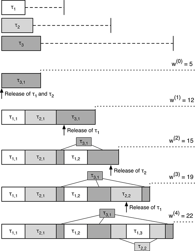
FIGURE 14.1
Scheduling sequence of the tasks of Table 14.1 and RTA analysis for task τ3.
TABLE 14.2
Worst-case response time for the sample task set
| Task τi | Period Ti | Computation Time Ci | Priority | Worst-Case Resp. Time Ri |
| τ1 | 8 | 3 | High | 3 |
| τ2 | 14 | 4 | Medium | 7 |
| τ3 | 22 | 5 | Low | 22 |
14.2 Computing the Worst-Case Execution Time
We have just seen how the worst-case response time can be derived by the knowledge of the task (fixed) priority assignment and from the worst-case execution time, that is, the time only due to the task in the worst case, without considering interference by higher-priority tasks.
The worst-case execution time can be obtained by two distinct methods often used in combination: measurement and analysis. Measurement is often easy to perform, but it may be difficult to be sure that the worst case has actually been observed. There are, in fact, several factors that may lead the production system to behave in a different way from the test system used for measurement.
For example, the task execution time can depend on its input data, or unexpected interference may arise, for example, due to the interrupts generated by some I/O device not considered in testing.
On the other side, analysis may produce a tight estimate of the worst-case execution time, but is more difficult to perform. It requires, in fact, an effective model of the processor (including pipelines, caches, memory, etc.) and sophisticated code analysis techniques. Moreover, as for testing, external factors not considered in analysis may arise in the real-world system. Most analysis techniques involve several distinct activities:
Decompose the code of the task into a directed graph of basic blocks. Each basic block is a straight segment of code (without tests, loops, and other conditional statements).
Consider each basic block and, by means of the processor model, determine its worst-case execution time.
Collapse the graph by means of the available semantic information about the program and, possibly, additional annotations provided by either the programmer or the compiler.
For example, the graph of an “if P then S1 else S2” statement can be collapsed into a single block whose worst-case execution time is equal to the maximum of the worst-case execution times of blocks S1 and S2. If that statement is enclosed in a loop to be executed 10 times, a straight estimation of the worst-case execution time would be derived by multiplying the worst-case execution time of the if block by 10. However, if it were possible to deduce, say, by means of more sophisticated analysis techniques, that the predicate P can be true on at the most three occasions, it would be possible to compute a more accurate overall worst-case execution time for the whole loop by multiplying the execution time of the block by 3.
Often, some restrictions must be placed on the structure of the code so that it can be safely analyzed to derive accurate values of its worst execution time. The biggest challenge in estimating worst execution time derives, however, from the influence of several hardware components commonly found in modern processors, whose intent is to increase computation throughput. These devices aim to reduce the average execution time, and normally perform very well in this respect. As a consequence, ignoring them makes the analysis very pessimistic. On the other hand, their impact on the worst-case execution time can be hard to predict and may sometimes be worse than in a basic system not using such mechanisms. In fact, in order to improve average performance, it may turn out more convenient to “sacrifice” performance in situations that seldom occur, in favor of others that happen more frequently. Average performance optimization methods, commonly used in modern processors, are Caches, Translation Lookaside Buffers, and Branch Prediction.
The cache consists of a fast memory, often mounted on the same processor chip, limited in size, which is intended to contain data most frequently accessed by the processor. Whenever a memory location is accessed, two possible situations arise:
The data item is found (cache hit) in the cache, and therefore, there is no need to access the external memory. Normally, the access is carried out in a single clock cycle.
The data item is not present in the cache (cache miss). In this case, the data item must be accessed in the external memory. At the same time, a set of contiguous data are read from the memory and stored in a portion of the cache (called cache line) so that the next time close data are accessed, they are found in the cache. The time required to handle a cache miss can be orders of magnitude larger than in a cache hit.
The performance of the cache heavily depends on the locality of memory access, that is, on the likelihood that accesses in memory are performed at contiguous addresses. This is indeed a common situation: program instructions are fetched in sequence unless code branches are performed, program variables are located on the stack at close addresses, and arrays are often accessed sequentially. It is, however, not possible to exclude situations in which a sequence of cache misses occurs, thus obtaining a worst-case execution time that is much larger than the average one. Therefore, even if it is possible to satisfactorily assess the performance of a cache from the statistical point of view, the behavior of a cache with respect to a specific data access is often hard to predict. Moreover, cache behavior depends in part on events external to the task under analysis, such as the allocation of cache lines due to memory accesses performed by other tasks.
Translation Lookaside Buffers (TLB) is a mechanism for speeding memory access in virtual memory systems. We have seen in Chapter 2 that virtual memory address translation implies a double memory access: a first access to the page table to get the address translation, and then to the selected memory page. As for cache access, very often memory access is local, and therefore, if a memory page has been recently accessed, then it is likely that it will be accessed again in a short time. For this reason, it is convenient to store in a small and fast associative memory the page translation information for a subset of the memory pages recently accessed to decrease overall memory access time. Observe that, in virtual memory systems, address translations is always performed when accessing memory regardless of the availability of the requested datum in the cache. If the page translation information is found in the TLB (TLB hit), there is no need to read the page table entry to get the physical page number. As for caches, even if the average performance is greatly improved, it is usually hard to predict whether a particular memory access will give rise to a TLB hit or to a miss. In the latter case, the memory access time may grow by an order of magnitude. Moreover, as for caches, TLB behavior depends in part on events external to the task under analysis. In particular, when a context switch occurs due, for example, to task preemption, the TLB is flushed because the virtual address translation is changed.
Branch prediction is a technique used to reduce the so-called “branch hazards” in pipelined processors. All modern processors adopt a pipelined organization, that is, the execution of the machine instructions is split into stages, and every stage is carried out by a separate pipeline component. The first stage consists in fetching the instruction code from the memory and, as soon as the instruction has been fetched, it is passed on to another element of the pipeline for decoding it, while the first pipeline component can start fetching in parallel the following instruction. After a startup time corresponding to the execution of the first instruction, all the pipeline components can work in parallel, obtaining a speed in overall throughput of a factor of N, where N is the number of components in the processor pipeline. Several facts inhibit, however, the ideal pipeline organization, and one of the main reason for this is due to the branch instructions. After a branch instruction is fetched from memory, the next one is fetched while the former starts being processed. However, if the branch condition turns out to be true (something that may be discovered some stages later), the following instructions that are being processed in the pipeline must be discarded because they refer to a wrong path in program execution. If it were possible to know in advance, as soon as a branch instruction is fetched, at what address the next instruction will be fetched (i.e., whether or not the branch will occur), there would be no need to flush the pipeline whenever the branch condition has been detected to be true. Modern processors use sophisticated techniques of branch prediction based on the past execution flow of the program, thus significantly reducing the average execution time. Prediction is, however, based on statistical assumptions, and therefore, prediction errors may occur, leading to the flush of the pipeline with an adverse impact on the task execution time.
The reader should be convinced at this point that, using analysis alone, it is in practice not possible to derive the worst-case execution time for modern processors. However, given that most real-time systems will be subject to considerable testing anyway, for example, for safety reasons, a combined approach that combines testing and measurement for basic blocks and path analysis for complete components can often be appropriate.
14.3 Aperiodic and Sporadic Tasks
Up to now we have considered only periodic tasks, where every task consists of an infinite sequence of identical activities called instances, or jobs, that are regularly released, or activated, at a constant rate.
A aperiodic task consists of an infinite sequence of identical jobs. However, unlike periodic tasks, their release does not take place at a regular rate. Typical examples of aperiodic asks are
User interaction. Events generated by user interaction (key pressed, mouse clicked) and which require some sort of system response.
Event reaction. External events, such as alarms, may be generated at unpredictable times whenever some condition either in the system or in the controlled plant occurs.
A aperiodic task for which it is possible to determine a minimum inter-arrival time interval is called a sporadic task. Sporadic tasks can model many situations that occur in practice. For example, a minimum interarrival time can be safely assumed for events generated by user interaction, because of the reaction time of the human brain, and, more in general, system events can be filtered in advance to ensure that, after the occurrence of a given event, no new instance will be issued until after a given dead time.
One simple way of expanding the basic process model to include sporadic tasks is to interpret the period Ti as the minimum interarrival time interval. Of course, much more sophisticated methods of handling sporadic tasks do exist, but their description is beyond the scope of an introductory textbook like this one. Interested readers are referred References [18, 19, 61] for a more comprehensive treatment of this topic.
For example, a sporadic task τi with Ti = 20 ms is guaranteed not to arrive more frequently than once in any 20 ms interval. Actually, it may arrive much less frequently, but a suitable schedulability analysis test will ensure (if passed) that the maximum rate can be sustained.
For these tasks, assuming Di = Ti, that is, a relative deadline equal to the minimum interarrival time, is unreasonable because they usually encapsulate error handlers or respond to alarms. The fault model of the system may state that the error routine will be invoked rarely but, when it is, it has a very short deadline. For many periodic tasks it is useful to define a deadline shorter than the period.
The RTA method just described is adequate for use with the extended process model just introduced, that is, when Di ≤ Ti. Observe that the method works with any fixed-priority ordering, and not just with the RM assignment, as long as the set hp(i) of tasks with priority larger than task τi is defined appropriately for all i and we use a preemptive scheduler. This fact is especially important to make the technique applicable also for sporadic tasks. In fact, even if RM was shown to be an optimal fixed-priority assignment scheme when Di = Ti, this is no longer true for Di ≤ Ti.
The following theorem (Leung and Whitehead, 1982) [59] introduces another fixed-priority assignment no more based on the period of the task but on their relative deadlines.
The deadline monotonic priority order (DMPO), in which each task has a fixed priority inversely proportional to its deadline, is optimum for a preemptive scheduler under the basic process model extended to let Di ≤ Ti.
The optimality of DMPO means that, if any task set Γ can be scheduled using a preemptive, fixed-priority scheduling algorithm A, then the same task set can also be scheduled using the DPMO. As before, such a priority assignment sounds to be good choice since it makes sense to give precedence to more “urgent” tasks. The formal proof of optimality will involve transforming the priorities of Γ (as assigned by A), until the priority ordering is Deadline Monotonic (DM). We will show that each transformation step will preserve schedulability.
Let τi and τj be two tasks in Γ, with adjacent priorities, that are in the wrong order for DMPO under the priority assignment schema A. That is, let Pi > Pj and Di > Dj under A, where Pi (Pj) denotes the priority of τi (τj). We shall define now a new priority assignment scheme A′ to be identical to A, except that the priorities of τi and τj are swapped and we prove that Γ is still schedulable under A′.
We observe first that all tasks with a priority higher than Pi (the maximum priority of the tasks being swapped) will be unaffected by the swap. All tasks with priorities lower than Pj (the minimum priority of the tasks being swapped) will be unaffected by the swap, too, because the amount of interference they experience from τi and τj is the same before and after the swap.
Task τj has a higher priority after the swap, and since it was schedulable, by hypothesis, under A, it will suffer after the swap either the same or less interference (due to the priority increase). Hence, it must be schedulable under A′, too. The most difficult step is to show now that task τi, which was schedulable under A and has had its priority lowered, is still schedulable under A′.
We observe first that once the tasks have been switched, the new worst-case response time of τi becomes equal to the old response time of τj, that is, .
Under the previous priority assignment A, we had
Rj ≤ Dj (schedulability)
Dj < Di (hypothesis)
Di ≤ Ti (hypothesis)
Hence, under A, τi only interferes once during the execution of τj because Rj < Ti, that is, during the worst-case execution time of τj, no new releases of τi can occur. Under both priority orderings, Ci +Cj amount of computation time is completed with the same amount of interference from higher-priority processes.
Under A′, since τj was released only once during , it interferes only once during the execution of τi. Therefore, we have
(just proved)
Rj ≤ Dj (schedulability under A)
Dj < Di (hypothesis)
Hence, , and it can be concluded that τi is still schedulable after the switch.
In conclusion, the DM priority assignment can be obtained from any other priority assignment by a sequence of pairwise priority reorderings as above. Each such reordering step preserves schedulability.
The following example illustrates a successful application of DMPO for a task set where RM priority assignment fails. Consider the task set listed in Table 14.3, where the RM and DM priority assignments differ for some tasks.
The behaviors of RM and DM for this task set will be now examined and compared.
From Figures 14.2 and 14.3 we can see that RM is unable to schedule the task set, whereas DM succeeds. We can derive the same result performing RTA analysis for the RM schedule.
For the RM schedule, we have, for τ3, hp(3) = ∅. Hence, R3 = C3 = 3, and τ3 (trivially) meets its deadline.
TABLE 14.3
RM and DM priority assignment
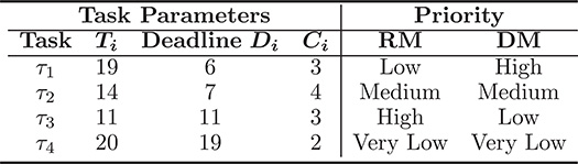
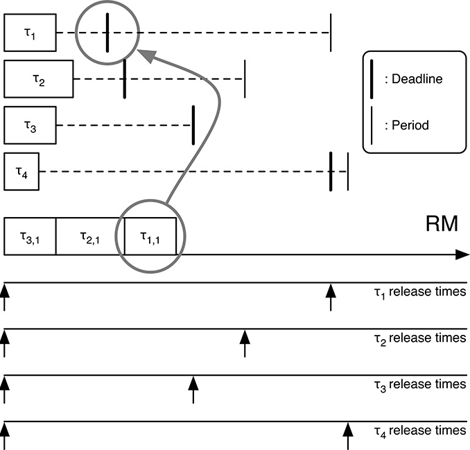
FIGURE 14.2
RM scheduling fails for the tasks of Table 14.3.
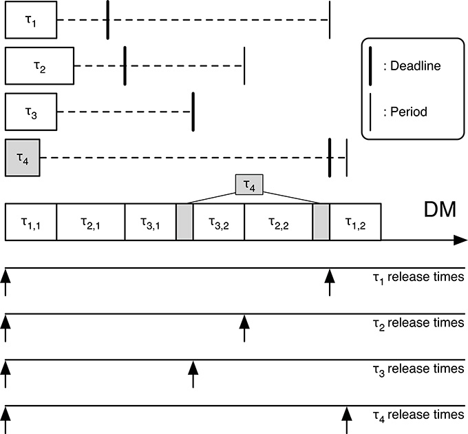
FIGURE 14.3
DM scheduling succeeds for the tasks of Table 14.3.
For τ2, hp(2) = {3} and:
Since R2 = 7 and D2 = 7, τ2 meets its deadline.
For τ1, hp(1) = {3, 2} and
Since R1 = 10 and D1 = 6, τ1 misses its deadline: RM is unable to schedule this task set.
Consider now RTA for the DM schedule: for τ1, hp(1) = ∅. Hence, R1 = C1 = 3, and τ1 (trivially) meets its deadline.
For τ2, hp(2) = {1} and
Since R2 = 7 and D2 = 7, τ2 just meets its deadline.
For τ3, hp(3) = {1, 2} and
Since R3 = 10 and D3 = 11, τ3 meets its deadline, too.
For τ4, hp(4) = {1, 2, 3} and
Finally, τ4 meets its deadline also because R4 = 19 and D4 = 19. This terminates the RTA analysis, proving the schedulability of Γ for the DM priority assignment.
14.4 Summary
This chapter introduced RTA, a check for schedulability that allows a finer resolution in respect of the other utilization-based checks. It is worth noting that, even when RTA fails, the task set may be schedulable because RTA assumes that all the tasks are released at the same critical instant. It is, however, always convenient and safer to consider the worst case (critical instant) in scheduling dynamics because it would be very hard to make sure that critical instants never occur due to the variability in the task execution time on computers, for example, to cache misses and pipeline hazards. Even if not so straight as the utilization-based check, RTA represents a practical schedulability check because, even in case of nonconvergence, it can be stopped as long as the currently computed response time for any task exceeds the task deadline.
The RTA method can be also be applied to Earliest Deadline First (EDF), but is considerably more complex than for the fixed-priority case and will not be considered in this book due its very limited applicability in practical application.
RTA is based on an estimation of the worst-case execution time for each considered task, and we have seen that the exact derivation of this parameter is not easy, especially for general-purpose processors, which adopt techniques for improving average execution speed, and for which the worst-case execution time can be orders of magnitude larger that the execution time in the large majority of the executions. In this case, basing schedulability analysis on the worst case may sacrifice most of the potentiality of the processor, with the risk of having a very low total utilization and, therefore, of wasting computer resources. On the other side, considering lower times may produce occasional, albeit rare, deadline misses, so a trade-off between deadline miss probability and efficient processor utilization is normally chosen. The applications where absolutely no deadline miss is acceptable are in fact not so common. For example, if the embedded system is used within a feedback loop, the effect of occasional deadline misses can be considered as a disturb (or noise) in either the controlled process, the detectors, or the actuators, and can be handled by the system, provided enough stability margin in achieved control.
Finally, RTA also allows dealing with the more general case in which the relative deadline Di for task τi is lower than the task period Ti. This is the case for sporadic jobs that model a set of system activities such as event and alarm handling. As a final remark, observe that, with the inclusion of sporadic tasks, we are moving toward a more realistic representation of real-time systems. The major abstraction so far is due to the task model, which assumes that tasks do not depend on each other, an assumption often not realistic. The next two chapters will cover this aspect, taking into account the effect due to the use of resources shared among tasks and the consequent effect in synchronization.