
20
Control Theory and Digital Signal Processing Primer
CONTENTS
20.1 Case Study: Controlling the Liquid Level in a Tank
20.1.1 The Use of Differential Equations to Describe the Dynamics of the System
20.1.2 Introducing an Integral Gain
20.1.3 Using Transfer Functions in the Laplace Domain
20.1.4 Deriving System Properties from Its Transfer Function
20.1.5 Implementing a Transfer Function
20.2 Case Study: Implementing a Digital low-pass Filter
20.2.1 Harmonics and the Fourier Transform
20.2.3 The Choice of the Sampling Period
20.2.4 Building the Digital Low-Pass Filter
Two case studies will be presented in this chapter in order to introduce basic concepts in Control Theory and Digital Signal Processing, respectively. The first one will consist in a simple control problem to regulate the flow of a liquid in a tank in order to stabilize its level. Here, some basic concepts of control theory will be introduced to let the reader become familiar with the concept of transfer function, system stability, and the techniques for its practical implementation.
The second case study is the implementation of a low-pass digital filter and is intended to introduce the reader to some basic concepts in digital signal processing, using the notation introduced by the first example.
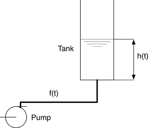
FIGURE 20.1
The tank–pump system.
20.1 Case Study 1: Controlling the Liquid Level in a Tank
Consider a tank containing a liquid and a pump that is able to move the liquid back and forth in the tank, as shown in Figure 20.1 The pump is able to generate a liquid flow and receives the flow reference from a control system with the aim of maintaining the level of the liquid in the tank to a given reference value, possibly varying over time. A practical application of such a system is the regulation of the fuel level inside the aircraft wings housing the fuel reservoir. The level of the fuel within each wing has to be maintained controlled in order to ensure the proper weight balancing in the aircraft during the flight and at the same time provide engine fueling.
The system has one detector for the measurement of the level of the liquid, producing a time-dependent signal representing, at every time t, the level h(t), and one actuator, that is, the pump whose flow at every time t depends on the preset value fp(t). In order to simplify the following discussion, we will assume that the pump represents an ideal actuator, producing a flow f (t) at any time equal to the current preset value, that is, f (t) = fp(t). The tank-pump system of Figure 20.1 will then have an input, that is, the preset flow f (t) and one output—the liquid level in the tank h(t). A positive value of f (t) means that the liquid is flowing into the tank, and a negative value of f (t) indicates that the liquid is being pumped away the tank. The tank–pump system input and output are correlated as follows:
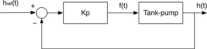
FIGURE 20.2
Tank–pump system controlled in feedback mode.
h(t)=h0+1B∫t0f(τ)dτ(20.1)(20.1)
where h0 is the level in the tank at time 0, and B is the base surface of the tank. f (τ)dτ represents, in fact, the liquid volume change during the infinitesimal time dτ. In order to control the level of the liquid, we may think of sending to the actuator (the pump) a reference signal that is proportional to the difference of the measured level and the reference level value, that is,
f(t)=Kp[href(t)-h(t)](20.2)(20.2)
corresponding to the schema shown in Figure 20.2. This is an example of feedback control where the reference signal depends also on its current output. Parameter Kp is called the Proportional Gain, and this kind of feedback control is called proportional because the system is fed by a signal which is proportional to the current error, that is, the difference between the desired output href (t) and the current one h(t). This kind of control intuitively works. In fact, if the current level h(t) is lower than the reference value href (t), the preset flow is positive, and therefore liquid enters the tank. Conversely, if h(t) > href (t), liquid is pumped away from the tank, and when the liquid level is ok, that is, h(t) = href (t), the requested flow is 0.
20.1.1 The Use of Differential Equations to Describe the Dynamics of the System
In order to compute the actual time evolution of the liquid level when, say, the reference value is set to href at time t = 0 and is not changed afterwards, and the initial level of the liquid is h0, we must consider the input/output (I/O) relationship of the tank-pump system of Figure 20.1, where the actual input is given by (20.2). From (20.1) we obtain
h(t)=h0+1B∫t0Kp[href-h(τ)]dτ(20.3)(20.3)
If we consider the time derivative of both terms in (20.3), we get
dh(t)dt=KpB[href-h(t)](20.4)(20.4)
that is, the differential equation
dh(t)dt+KpBh(t)=KpBhref(20.5)(20.5)
whose solution is the actual evolution h(t) of the liquid level in the tank.
The tank–pump system is an example of linear system. More in general, the I/O relationship for linear systems is expressed by the differential equation
andyndtn+an-1dyn-1dtn-1+…+a1dydt+a0=bmdumdtm+bm-1dum-1dtm-1+…+b1dudt+b0(20.6)(20.6)
where u(t) and y(t) are the input and output of the system, respectively, and coefficients ai and bi are constant. In our tank–pump system, the input u(t) is represented by the applied reference level href (t) and the output y(t) is the actual liquid level h(t). The general solution of the above equation is of the form
y(t)=yl(t)+yf(t)(20.7)(20.7)
where yl(t) is the homogeneous solution, that is, the solution of the same differential equation, where the term on the right is 0 and describes the free evolution of the system, and yf (t) is a particular solution of (20.6), also called forced evolution. In our case, the reference href is constant, and therefore, a possible choice for the forced evolution is yf (t) = href. In this case, in fact, for t > 0, the derivative term of (20.5) is 0, and the equation is satisfied.
In order to find the homogeneous solution, we recall that the general solution of the generic differential equation
andyndtn+an-1dyn-1dtn-1+…+a1dydt+a0=0(20.8)(20.8)
is of the form
y(t)=n′∑i=1μi∑k=0Aiktkepit(20.9)(20.9)
where Aik are coefficients that depend on the initial system condition, and n′ and μi are the number of different roots and their multiplicity of the polynomial
anpn+an-1pn-1+…+a1p+a0=0(20.10)(20.10)
respectively. Polynomial (20.10) is called the characteristic equation of the differential equation (20.7). The terms tkepit are called the modes of the system. Often, the roots of (20.10) have single multiplicity, and the modes are then of the form epit. It is worth noting that the roots of polynomial (20.10) may be real values or complex ones, that is, of the form p = a + jb, where a and b are the real and imaginary parts of p, respectively. Complex roots (20.10) appear in conjugate pairs (the conjugate of a complex number a+jb is a−jb). We recall also that the exponential of a complex number p = a + jb is of the form ep = ea[cos b + j sin b]. The modes are very important in describing the dynamics of the system. In fact, if any root of the associated polynomial has a positive real part, the corresponding mode will have a term that diverges over time (an exponential function with an increasing positive argument), and the system becomes unstable. Conversely, if all the modes have negative real part, the system transients will become negligible after a given amount of time. Moreover, the characteristics of the modes of the system provide us with additional information. If the modes are real numbers, they have the shape of an exponential function; if instead they have a nonnull imaginary part, the modes will have also an oscillating term, whose frequency is related to the imaginary part and whose amplitude depends on the real part of the corresponding root.
The attentive reader may be concerned by the fact that, while the modes are represented by complex numbers, the free evolution of the system must be represented by real numbers (after all, we live in a real world). This apparent contradiction is explained by considering that the complex roots of (20.10) are always in conjugate pairs, and therefore, the imaginary terms elide in the final summation of (20.9). In fact, for every complex number p = a + jb and its complex conjugate ˉp=a−jb
eˉp=ea[cos(b)+jsin(-b)]=ea[cos(b)-jsin(b)]=¯(ep);(20.11)(20.11)
moreover, considering the common case in which solutions of the characteristic equation have single multiplicity, the (complex) coefficients Ai in (20.9) associated with pi = a + jb and ¯pi=a−jb
Aiepit+¯Aie¯pit=ea[2Re(Ai)cos(bt)-2Im(Ai)sin(bt)](20.12)(20.12)
where Re(Ai) and Im(Ai) are the real and imaginary parts of Ai, respectively. Equation (20.12) represents the contribution of the pair of conjugate roots, which is a real number.
Coming back to our tank–pump system, the polynomial associated with the differential equation describing the dynamics of the system is
p+KpB=0(20.13)(20.13)
which yields the single real solution p0=−KpB
hl(t)=Ae-KptB(20.14)(20.14)
and the general solution for (20.5) is
h(t)=hl(t)+hf(t)=Ae-KptB+href(20.15)(20.15)
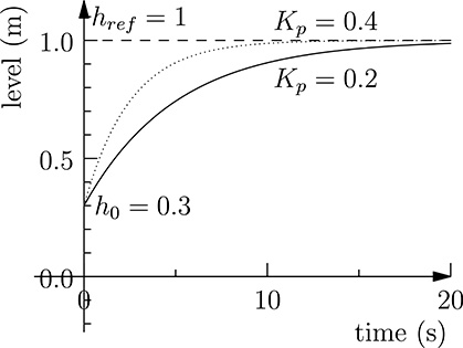
FIGURE 20.3
Tank–pump system response when controlled in feedback mode.
where hl(t) and hf(t) are the free and forced solutions of (20.5).
Parameter A is finally computed considering the boundary condition of the system, that is, the values of h(t) for t = 0−. Just before the reference value href has been applied to the system. For t = 0− (20.15) becomes
h0=Ae0+href=A+href(20.16)(20.16)
which yields the solution A = h0 − href, thus getting the final response of our tank–pump system
h(t)=(h0-href)e-KptB+href(20.17)(20.17)
The system response of the tank–pump system controlled in feedback, that is, the time evolution of the level of the liquid in the tank in response to a step reference href is shown in Figure (20.3) for two different values of the proportional gain Kp, with tank base surface B = 1m2.
20.1.2 Introducing an Integral Gain
We observe that the proportional gain Kp affects the readiness of the response, as shown by Figure 20.3, and larger proportional gains produce a faster response. We may therefore think that we can choose a proportional gain large enough to reach the desired speed in the response. However, in the choice of Kp we must consider the limit in the pump ability in generating the requested liquid flow. As an example, the flow request to the pump at the proportional gains considered in Figure 20.3, is shown in Figure 20.4.
From Figure 20.4 it can be seen that larger proportional gains imply larger flows requested to the pump. In practice, the maximum allowable value of the proportional gain is limited by the maximum flow the pump is able to generate. Moreover, the system will always approach the requested liquid level asymptotically. We may wonder if it is possible to find some other control schema that could provide a faster response. A possibility could be considering an additional term in the input for the pump that is proportional to the integral of the error, in the hope it can provide a faster response. In fact, in the evolution plotted in Figure 20.3, the integral of the error is always positive. We may expect that forcing the integral of the error to become null will provide a faster step response, possibly with an overshoot, in order to make the overall error integral equal to 0 (see Figure 20.9). To prove our intuition, we consider a reference signal for the pump of the form
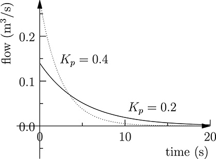
FIGURE 20.4
Flow request to the pump using feedback control with proportional gain.
f(t)=Kp[href(t)-h(t)]+Ki∫t0[href(τ)-h(τ)]dτ(20.18)(20.18)
where Kp and Ki are the proportional and integral gains in the feedback control, respectively. We obtain, therefore, the relation
h(t)=h0+1B∫t0f(τ)dτ=h0+1B∫t0{Kp[href(τ)-h(τ)]+KiB∫τ0[href(τ′)-h(τ′)]dτ′}dτ(20.19)
Derivating both terms, we obtain
dh(t)dt=KpB[href(t)-h(t)]+KiB∫t0[href(τ)-h(τ)]dτ(20.20)(20.20)
and, by derivating again
d2h(t)dt2=KpB[dhref(t)dt-dh(t)dt]+KiB[href(t)-h(t)](20.21)(20.21)
that is, the differential equation
Bd2h(t)dt2+Kpdh(t)dt+Kih(t)=Kihref(t)+Kpdhref(t)dt(20.22)(20.22)
whose solution is the time evolution h(t) of the liquid level in the tank.
20.1.3 Using Transfer Functions in the Laplace Domain
At this point the reader may wonder if defining control strategies always means solving differential equations, which is possibly complicated. Fortunately, this is not the case, and control theory uses a formalism for describing linear systems that permits the definition of optimal control strategies without developing explicit solutions to the differential equations representing the I/O relationship.
Instead of dealing with time-dependent signals, we shall use Laplace transforms. Given a function on time f (t), its Laplace transform is of the form
F(s)=L{f(t)}=∫∞0f(t)e-stdt(20.23)(20.23)
where s and F(s) are complex numbers. Even if at a first glance this approach may complicate things, rather than simplifying problems (we are now considering complex functions of complex variables), this new formalism can rely on a few interesting properties of the Laplace transforms, which turn out to be very useful for expressing I/O relationships in linear systems in a simple way. In particular we have
L{Af(t)+Bg(t)}=AL{f(t)}+BL{g(t)}(20.24)(20.24)
L{df(t)dt}=sL{f(t)}(20.25)(20.25)
L{∫f(t)dt}=L{f(t)}s(20.26)(20.26)
Equation (20.24) states that the Laplace transform is a linear operator, and, due to (20.25) and (20.26), relations expressed by time integration and derivation become algebraic relations when considering Laplace transforms. In the differential equation in (20.22), if we consider the Laplace transforms H(s) and Href(s) in place of h(t) and href(t), from (20.24), (20.25) and (20.26), we have for the tank–pump system
Bs2H(s)+KpsH(s)+KiH(s)=KiHref(s)+KpsHref(s)(20.27)(20.27)
that is,
H(s)=Ki+KpsBs2+Kps+KiHref(s)(20.28)(20.28)
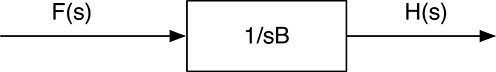
FIGURE 20.5
Graphical representation of the transfer function for the tank–pump system.
Observe that the I/O relationship of our tank–pump system, which is expressed in the time domain by a differential equation, becomes an algebraic relation in the Laplace domain. The term
W(s)=Ki+KpsBs2+Kps+Ki(20.29)(20.29)
is called the Transfer Function and fully characterizes the system behavior. Using Laplace transforms, it is not necessary to explicitly express the differential equation describing the system behavior, and the transfer function can be directly derived from the block description of the system. In fact, recalling the I/O relationship of the tank and relating the actual liquid level h(t) and the pump flow f(t) in (20.1), using property (20.26),we can express the same relationship in the Laplace domain as
H(s)=1sBF(s)(20.30)(20.30)
where H(s) and F(s) are the Laplace transforms of h(t) and f(t), respectively. This relation can be expressed graphically as in Figure 20.5. Considering the control law involving the proportional and integral gain
f(t)=Kp[href(t)-h(t)]+Ki∫t0[href(τ)-h(τ)]dτ(20.31)(20.31)
the same law expressed in the Laplace domain becomes:
F(s)=(Kp+Kis)[Href(s)-H(s)](20.32)(20.32)
and therefore, we can express the whole tank–pump system as in Figure 20.6. From that figure we can easily derive
H(s)=1sB[Kp+Kis][Href(s)-H(s)](20.33)(20.33)
that is
H(s)=Href(s)sKp+Kis2B+sKp+Ki(20.34)(20.34)
obtaining, therefore, the same transfer function of (20.29) directly from the graphical representation of the system without explicitly stating the differential equation describing the system dynamics.
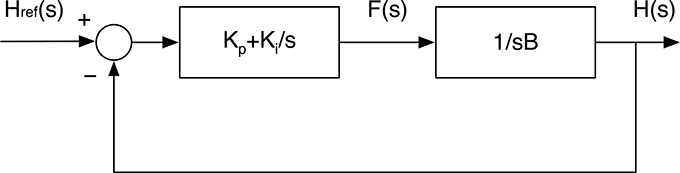
FIGURE 20.6
Graphical representation of tank–pump system controlled in feedback.
20.1.4 Deriving System Properties from Its Transfer Function
The transfer function W(s) of a linear system fully describes its behavior and, in principle, given any reference href(t), we could compute its Laplace transform, multiply it for W(s), and then compute its antitransform to retrieve the system response h(t). We do not report here the formula for the Laplace antitransform because, in practice, an analytical solution of the above procedure would be very difficult, if not impossible. Rather, computational tools for the numerical simulation of the system behavior are used by control engineers in the development of optimal control strategies. Several important system properties can, however, be inferred from the transfer function W (s) without explicitly computing the system evolution over time. In particular, stability can be inferred from W (s) when expressed in the form
W(s)=N(s)D(s)(20.35)(20.35)
The roots of N (s) are called the zeroes of the transfer function, while the roots of D(s) are called the poles of the transfer function. W (s) becomes null in its zeroes, diverging when s approaches its poles. Recall that W (s) is a complex value of complex variable. For a graphical representation of W (s), usually its module is considered. Recall that the module of a complex number √a2+b2
The function shown in Figure 20.7 diverges when s approaches the roots of D(s) = s2 + s + 1, i.e., for s1=−12+j√32
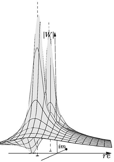
FIGURE 20.7
The module of the transfer function for the tank–pump system.
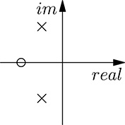
FIGURE 20.8
Zeroes and poles of the transfer function for the tank–pump system.
becomes null when N (s) = 0, that is, for s = −1 + j0. There is normally no need to represent graphically in this way the module of the transfer function W (s), and it is more useful to express graphically its poles and zeroes in the complex plane, as shown in Figure 20.8. By convention, zeroes are represented by a circle and poles by a cross. System stability can be inferred by W (s) when expressed in the form W(s)=N(s)D(s)
Let us now return to the tank–pump system controlled in feedback using a proportional gain, Kp, and an integral gain, Ki. Recalling its transfer function in (20.34), we observe that its poles are the solution to equation
s2B+sKp+Ki=0(20.36)(20.36)
that is,
s1,2=-Kp±√K2p-4KiB2B(20.37)(20.37)
(recall that B is the base surface of the tank). Figure 20.9 shows the controlled tank–pump response for Kp = 0.4 and Ki = 0.02, compared with the same response for a proportional gain Kp = 0.4 only. It can be seen that the response is faster, but an overshoot is present, as the consequence of the nonnull integral gain (recall that control tries to reduce the integral of the error in addition to the error itself). For Kp>2√KiB
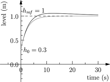
FIGURE 20.9
The response of the controlled tank–pump system with proportional gain set to 0.4 and integral gains set to 0.02 (black) and 0 (grey), respectively.
Before proceeding, it is worthwhile now to summarize the advantages provided by the representation of the transfer functions expressed in the Laplace domain for the analysis of linear systems. We have seen how it is possible to derive several system properties simply based on its block diagram representation and without deriving the differential equation describing the system dynamics. More importantly, this can be done without deriving any analytical solution of such differential equation. This is the reason why this formalism is ubiquitously used in control engineering.
20.1.5 Implementing a Transfer Function
So far, we have learned some important concepts of control theory and obtained some insight in the control engineer’s duty, that is, identifying the system, modeling it, and finding a control strategy. The outcome of this task is the specification of the control function, often expressed in the Laplace domain. It is worth noting that in the definition of the control strategy for a given system, we may deal with different transfer functions. For example, in the tank–pump system used throughout this chapter, we had the following transfer functions:
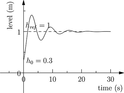
FIGURE 20.10
The response of the controlled tank–pump system with proportional gain set to 0.4 and integral gain set to 1.
W1(s)=1Bs(20.38)(20.38)
which is the description of the tank I/O relationship
W2(s)=Kp+Kis(20.39)(20.39)
which represents the control law, and
W3(s)=Ki+KpsBs2+Kps+Ki(20.40)(20.40)
which describes the overall system response.
If we turn our attention to the implementation of the control, once the parameters Kp and Ki have been chosen, we observe that the embedded system must implement W2(s), that is, the controller. It is necessary to provide to the controller the input error href (t) − h(t), that is the difference between the current level of the liquid in the tank and the reference one. The output of the controller, f (t) will drive the pump in order to provide the requested flow. The input to the controller is therefore provided by a sensor, while its output will be sent to an actuator. The signals h(t) and f (t) may be analog signals, such as a voltage level. This was the common case in the older times, prior to the advent of digital controllers. In this case the controller itself was implemented by an analog electronic circuit whose I/O law corresponded to the desired transfer function for control. Nowadays, analog controllers are rarely used and digital controllers are used instead. Digital controllers operate on the sampled values of the input signals and produce sampled outputs. The input may derive from analog-to-digital conversion (ADC) performed on the signal coming from the sensors, or taking directly the numerical values from the sensor, connected via a local bus, a Local Area Network or, more recently, a wireless connection. The digital controller’s outputs can then be converted to analog voltages by means of a Digital to Analog converter (DAC) and then given to the actuators, or directly sent to digital actuators with some sort of bus interface.
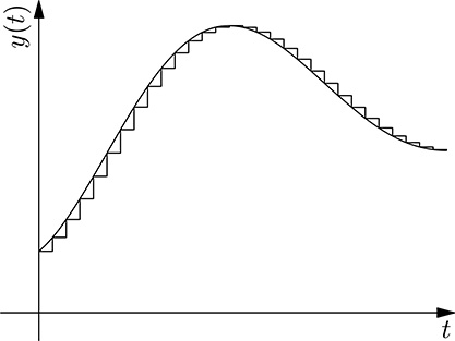
FIGURE 20.11
Sampling a continuous function.
When dealing with digital values, that is, the sampled values of the I/O signals, an important factor is the sampling period T. For the tank–pump system, the analog input h(t) is then transformed into a sequence of sampled values h(nT) as shown in Figure 20.11. Since sampling introduces unavoidable loss of information, we would like that the sampled signal could represent an approximation that is accurate enough for our purposes. Of course, the shorter the sampling period T, the more accurate the representation of the original analog signal. On the other side, higher sampling speed comes at a cost since it requires a faster controller and, above all, faster communication, which may become expensive. A trade-off is therefore desirable, that is, choosing a value of T that is short enough to get an acceptable approximation, but avoiding implementing an “overkill.” Such a value of T cannot be defined a priori, but depends on the dynamics of the system; the faster the system response, the shorted must be the sampling period T. A crude method for guessing an appropriate value of T is to consider the step response of the system, as shown in (20.9), and to choose T as the rise time divided for 10, so that a sufficient number of samples can describe the variation of the system output. More accurate methods consider the poles of W (s), which determine the modes of the free system evolution, that is, its dynamics. In principle, the poles with the largest absolute value of their real part, that is, describing the fastest modes of the system, should be considered, but they are not always significant for control purposes (for example, when their contribution to the overall system response is negligible). Moreover, what gets digitized in the system is only the controller, not the system itself. For this reason, normally the working range of frequencies for the controller is considered, and the sampling period chosen accordingly. The second test case presented in this chapter will describe more in detail how the sampling period is chosen based on frequency information.
Before proceeding further, it is necessary to introduce another mathematical formalism that turns out very useful in digitalizing transfer functions, and, in the end, in implementing digital controllers: the Z transform. Given a sequence of real values y(n), its Z transform is a complex function of complex variable z defined as
Z{y(n)}=∞∑n=-∞y(n)z-n(20.41)(20.41)
Even if this may seem another way to complicate the engineer’s life (as for the Laplace transforms, we are moving from the old, familiar, real space into a complex one), we shall see shortly how Z transforms are useful for specifying the I/O relationship in digital controllers. The following important two facts hold:
Z{Ay1(n)+By2(n)}=AZ{y1(n)}+BZ{y2(n)}(20.42)(20.42)
that is, the Z transform is linear, and
Z{y(n-1)}=∞∑n=-∞y(n-1)z-n=∞∑n′=-∞y(n′)z-n′z-1=z-1Z{y(n)}(20.43)(20.43)
The above relation has been obtained by replacing the term n in the summation with n′ = n − 1. Stated in words, (20.43) means that there is a simple relation (the multiplication for z−1) between the Z transform of a sequence y(n) and that of the same sequence delayed of one sample. Let us recall the general I/O relationship in a linear system:
andyndtn+an-1dyn-1dtn-1+…+a1dydt+a0=bmdumdtm+bm-1dum-1dtm-1+…+b1dudt+b0(20.44)(20.44)
where u(t) and y(t) are the continuous input and output of the system, respectively. If we move from the continuous values of y(t) and u(t) to the corresponding sequence of sampled values y(kT ) and u(kT ), after having chosen a period T small enough to provide a satisfactory approximation of the system evolution, we need to compute an approximation of the sampled time derivatives of y(t) and u(t). This is obtained by approximating the first order derivative with a finite difference:
dydt(kT)≃y(kT)-y((k-1)T)T(20.45)(20.45)
Recalling that the Z transform is linear, we obtain the following Z representation of the first-order time-derivative approximation:
Z{y(kT)-y((k-1)T)T}=1TZ{y(kT)}-z-1TZ{y(kT)}=1-z-1TZ{y(kT)}(20.46)(20.46)
which is a relation similar to that of (20.25) relating the Laplace transforms of y(t) and its time derivative expressing the I/O relationship for a linear system. Using the same reasoning, the second-order time derivative is approximated as (
(1-z-1T)2Z{y(kT)}(20.47)(20.47)
The I/O relationship expressed using Z transforms then becomes
Y(z)[an(1-z-1)nTn++a1(1-z-1)T+a0]=U(z)[bm(1-z-1)mTm++b1(1-z-1)T+b0](20.48)(20.48)
that is,
Y(z)=V(z)U(z)(20.49)(20.49)
where Y (z) and U (z) are the Z transform of y(t) and u(t), respectively, and V (z) is the transfer function of the linear system in the Z domain. Again, we obtain an algebraic relationship between the transforms of the input and output, considering the sampled values of a linear system. Observe that the transfer function V (z) can be derived directly from the transfer function W (s) in the Laplace domain, by the replacement
s=1−z−1T(20.50)(20.50)
From a specification of the transfer function W (s) expressed in the form W(s)=N(s)D(s)
V(z)=∑mi=0bi(z-1)i∑ni=0ai(z-1)i(20.51)(20.51)
that is,
Y(z)n∑i=0ai(z-1)i=U(z)m∑i=0bi(z-1)i(20.52)(20.52)
Recalling that Y (z)z−1 is the Z transform of the sequence y((k − 1)T ) and, more in general, that Y (z)z−i is the Z transform of the sequence y((k − i)T ), we can finally get the I/O relationship of the discretized linear system in the form
n∑i=0aiy((k-i)T)=m∑i=0biu((k-i)T)(20.53)(20.53)
that is,
y(kT)=1a0[m∑i=0biu((k-i)T)-(n∑i=1aiy((k-i)T)](20.54)(20.54)
Put in words, the system output is the linear combination of the n−1 previous outputs and the current input plus the m − 1 previous inputs. This representation of the controller behavior can then be easily implemented by a program making only multiplication and summations, operations that can be executed efficiently by CPUs.
In summary, the steps required to transform the controller specification given as a transfer function W (s) into a sequence of summations and multiplications are the following:
Find out a reasonable value of the sampling period T. Some insight into the system dynamics is required for a good choice.
Transform W (s) into V (z), that is, the transfer function of the same system in the Z domain by replacing variable s with 1−z−1T
1−z−1T .From the expression of V (z) as the ratio of two polynomials in z−1, derive the relation between the current system output y(kT ) and the previous input and output history.
Returning to the case study used through this section, we can derive the implementation of the digital controller for the tank–pump system from the definition of its transfer function in the Laplace domain, that is,
W2(s)=sKp+Kis(20.55)(20.55)
representing the proportional and integral gain in the feedback control. Replacing s with 1−z−1T
V(z)=Kp+KiT-z-1Kp1-z-1(20.56)(20.56)
from which we derive the definition of the algorithm
y(kT)=y((k-1)T+(Kp+KiT)u(kT)-Kpu((k-1)T)(20.57)(20.57)
where the input u(kT ) is represented by the sampled values of the difference between the sampled reference href (kT ) and the actual liquid level h(kT ), and the output y(kT ) corresponds to the flow reference sent to the pump.
Observe that the same technique can be used in a simulation tool to compute the overall system response, given the transfer function W (s). For example, the plots in Figures (20.9) and (20.10) have been obtained by discretizing the overall tank–pump transfer function (20.40).
An alternative method for the digital implementation of the control transfer function is the usage of the Bilinear Transform, that is, using the replacement
s=2T1-z-11+z-1(20.58)(20.58)
which can be derived from the general differential equation describing the linear system using a reasoning similar to that used to derive (20.50).
20.1.6 What We Have Learned
Before proceeding to the next section introducing other important concepts for embedded system development, it is worthwhile to briefly summarize the concepts that have been presented here. First of all, an example of linear system has been presented. Linear systems represent a mathematical representation of many practical control applications.We have then seen how differential equations describe the dynamics of linear systems. Even using a very simple example, we have experienced the practical difficulty in finding solutions to differential equations. The definition and some important concepts of the Laplace transform have been then presented, and we have learned how to build a transfer function W (s) for a given system starting from its individual components. Moreover, we have learned how it is possible to derive some important system characteristics directly from the transfer function W (s), such as system stability. Finally, we have learned how to implement in practice the I/O relationship expressed by a transfer function.
It is useful to highlight what we have not learned here. In fact, control theory is a vast discipline, and the presented concepts represent only just a very limited introduction. For example, no technique has been presented for finding the optimal proportional and integral gains, nor we have explored different control strategies. Moreover, we have restricted our attention to systems with a single-input and a single-output (SISO systems). Real-world systems, however, may have multiple inputs and multiple outputs (MIMO systems), and require more sophisticated mathematical techniques involving linear algebra concepts.
It is also worth stressing the fact that even the most elegant and efficient implementation can fail if the underlying algorithm is not correct, leading, for example, to an unstable system. So, it is often very important that an accurate analysis of the system is carried out in order to find a good control algorithm. The transfer function of the digital controller should also be implemented in such a way that its parameters can be easily changed. Very often, in fact, some fine tuning is required during the commissioning of the system.
As a final observation, all the theory presented here and used in practice rely on the assumption that the system being controlled can be modeled as a linear system. Unfortunately, many real-world systems are not linear, even simple ones. In this case, it is necessary to adopt techniques for approximating the nonlinear systems with a linear one in a restricted range of parameters of interest.
20.2 Case Study 2: Implementing a Digital low-pass Filter
In the previous section we have introduced the Laplace transform, that is, a transformation of a real function defined over time y(t), representing in our examples the time evolution of the signals handled by the control system, into a complex function Y (s) of a complex variable. In this section we present another powerful and widely used transformation that converts the time evolution of a signal into its representation in the frequency domain.
20.2.1 Harmonics and the Fourier Transform
In order to better understand what we intend for frequency domain, let us introduce the harmonics concept. A harmonic function is of the form
y(t)=Acos(2Πft+ϑ)(20.59)(20.59)
that is, a sinusoidal signal of amplitude A, frequency f, and phase ϑ. Its period T is the inverse of the frequency, that is, T=1f
can be expressed by the following Fourier series:
fsquare(t)=4Π∞∑k=1cos(2Π(2k-1)t-Π2)2k-1(20.60)(20.60)
Each harmonic is represented by a sinusoidal signal of frequency f = 2k − 1, phase ϑ=−π2
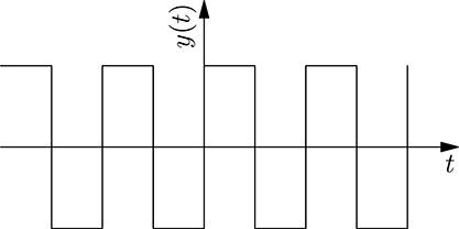
FIGURE 20.12
A square function.
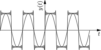
FIGURE 20.13
The approximation of a square function considering 1 and 10 harmonics.
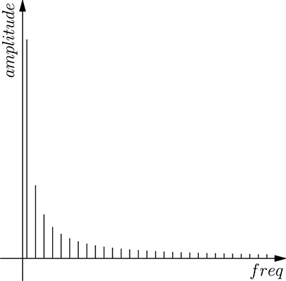
FIGURE 20.14
The components (amplitude vs. frequency) of the harmonics of the square function.
In the general case, the representation of a function y(t) in the frequency domain is mathematically formalized by the Fourier transform, which converts a signal y(t) expressed in the time domain into its representation in the frequency domain, that is, a complex function of real variable of the form
F{y(t)}=Y(f)=∫∞-∞y(t)e-j2Πftdt(20.61)(20.61)
Recall that, due to Eulero’s formula,
e-j2Πft=cos(2Πft)-jsin(2Πft)(20.62)(20.62)
The reader may wonder why the Fourier transform yields a complex value.
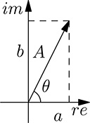
FIGURE 20.15
Representation of a complex number in the re–im plane.
Intuitively, this is because for every frequency f, the corresponding harmonics is characterized by two parameters: its amplitude and its phase. Given a frequency value f1, we shall see that the corresponding value of the Fourier transform Y (f1) is a complex number whose module and phase represent the amplitude and the phase of the corresponding harmonic. Recall that for a complex number a + jb, its module is A=√a2+b2
Informally stated, the Fourier transform represents, for every given frequency f, the (infinitesimal) contribution of the corresponding harmonic to function y(t). We can better understand this concept considering the inverse Fourier transform, that is, the transformation from Y (f ) = F {y(t)} into y(t):
y(t)=∫∞-∞F(f)ej2Πftdf(20.63)(20.63)
In words, every infinitesimal contribution F (f )ej2πf tdf represents the contribution of the harmonic at frequency f whose amplitude and phase correspond to the module and phase of F (f ), respectively. This may seem not so intuitive (we are considering the product between two complex numbers), but it can be easily proven as follows.
Consider a given frequency value f1. For this value, the Fourier transform yields Y (f1), which is a complex number of the form a+jb. From Figure 20.15 we can express the same complex number as
Y(f1)=a+jb=A[cosθ+jsinθ]=Aejθ(20.64)(20.64)
Where A=√a2+b2
Y(f1)ej2Πft1+Y(-f1)e-j2Πft1(20.65)(20.65)
A property of the Fourier transform Y (f ) of a real function y(t) is that Y (−f ) is the complex conjugate of Y (f ), and therefore, for the Eulero’s formula, if Y (f ) = Aejθ, then Y (−f ) = Ae−jθ. We can then rewrite (20.65) as
Aejθej2Πft1+Ae-jθe-j2Πft1=A[ej2Πft+θ1+e-j2Πft+θ1](20.66)(20.66)
The imaginary terms in (20.66) elide, and therefore,
Y(f1)ej2Πft1+Y(-f1)e-j2Πft1=2Acos(2Πf1t+θ)(20.67)(20.67)
That is, the contribution of the Fourier transform Y (f ) at the given frequency f1 is the harmonic at frequency f1 whose amplitude and phase are given by the module and phase of the complex number Y (f1).
Usually, the module of the Fourier transform Y (f ) is plotted against frequency f to show the frequency distribution of a given function f (t). The plot is symmetrical in respect of the Y axis. In fact, we have already seen that Y(−f)=¯Y(f)
The concepts we have learned so far are can be applied to a familiar concept, that is, sound. Intuitively, we expect that grave sounds will have a harmonic content mostly containing low frequency components, while acute sounds will contain harmonic components at higher frequencies. In any case, the sound we perceive will have no harmonics over a given frequency value because our ear is not able to perceive sounds over a given frequency limit.
20.2.2 Low-Pass Filters
A low-pass filter operates a transformation over the incoming signal so that frequencies above a given threshold are removed. Low-pass filters are useful, for example, to remove noise from signals. In fact, the noise has a frequency distribution where most components are above the frequencies of interest for the signal. A filter able to remove high frequency components will then remove most of the noise from the signal. As an example, consider Figure 20.16 showing a noisy signal. Its frequency distribution (spectrum) is shown in Figure 20.17, where it can be shown that harmonics are present at frequencies higher than 5Hz. Filtering the signal with a low-pass filter that removes frequencies above 5Hz, we get the signal shown in Figure 20.18, whose spectrum is shown in Figure 20.19. It can be seen that the frequencies above 5Hz have been removed thus removing the noise superimposed to the original signal.
The ideal low-pass filter will completely remove all the harmonics above a given cut-off frequency, leaving harmonics with lower frequency as they are. So the frequency response of the ideal low-pass frequency filter with cut-off frequency fc would have the form shown in Figure 20.20, where, in the Y axis, the ratio between the amplitudes of the original and filtered harmonics is shown. In practice, however, it is not possible to implement low-pass filters with such a frequency response. For example, the frequency response of the low-pass filter used to filter the signal shown in Figure 20.16 is shown in Figure 20.21. The gain of the filter is normally expressed in decibel (dB), corresponding to 20 log10 (A1/A0), where A0 and A1 are the amplitude of the original and filtered harmonic, respectively. Since the gain is normally less than or equal to one for filters, its expression in decibel is normally negative. The frequency response shown in Figure 20.21 is shown expressed in decibel in Figure 20.22. Referring to Figure 20.21, for frequencies included in the Pass Band the gain of the filter is above a given threshold, normally −3dB (in the ideal filter the gain in the pass band is exactly 0 dB), while in the Stop Band the gain is below another threshold, which, depending on the application, may range from −20 dB and −120 dB (in the ideal filter the gain in decibel for these frequencies tends to −∞). The range of frequencies between the pass band and the stop band is often called transition band: for an ideal low-pass filter there is no Transition Band, but in practice the transition band depends on the kind of selected filters, and its width is never null.
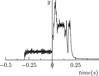
FIGURE 20.16
A signal with noise.
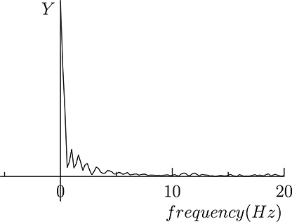
FIGURE 20.17
The spectrum of the signal shown in Figure (20.16).
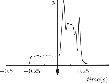
FIGURE 20.18
The signal of Figure 20.16 after low-pass filtering.
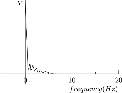
FIGURE 20.19
The spectrum of the signal shown in Figure 20.18.
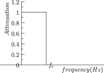
FIGURE 20.20
Frequency response of an ideal filter with cut-off frequency fc.
A low-pass filter is a linear system whose relationship between the input (unfiltered) signal and the output (filtered) one is expressed by a differential function in the form of (20.6). We have already in hand some techniques for handling linear systems and, in particular, we know how to express the I/O relationship using a transfer function W (s) expressed in the Laplace domain. At this point, we are able to recognize a very interesting aspect of the Laplace transform. Recalling the expression of the Laplace transform of function w(t)
W(s)=∫∞0w(t)e-stdt(20.68)(20.68)
and of the Fourier transform
W(f)=∫∞-∞w(t)e-2Πftdt(20.69)(20.69)
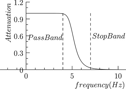
FIGURE 20.21
Frequency response of the filter used to filter the signal shown in Figure 20.16.
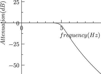
FIGURE 20.22
Frequency response shown in Figure 20.21 expressed in decibel.
and supposing that f (t) = 0 before time 0, the Fourier transform corresponds to the Laplace one, for s = j2πf, that is, when considering the values of the complex variable s corresponding to the imaginary axis. So, information carried by the Laplace transform covers also the frequency response of the system. Recalling the relationship between the input signal u(t) and the output signal y(t) for a linear system expressed in the Laplace domain
Y(s)=W(s)U(s)(20.70)(20.70)
we get an analog relationship between the Fourier transform U (f ) and Y (f ) of the input and output, respectively:
Y(f)=W(f)U(f)(20.71)(20.71)
In particular, if we apply a sinusoidal input function u(t) = cos(2πf t), the output will be of the form y(t) = A cos (2πf t + θ), where A and θ are the module and phase of W (s), s = ej2πf.
Let us consider again the transfer function of the tank–pump with feedback control we defined in the previous section. We recall here its expression
W(s)=sKp+Kis2B+sKp+Ki(20.72)(20.72)
Figure 20.23 shows the module of the transfer function for B = 1, Kp = 1, and Ki = 1, and, in particular, its values along the imaginary axis. The corresponding Fourier transform is shown in Figure 20.24. We observe that the tank–pump system controlled in feedback mode behaves somewhat like a low-pass filter. This should not be surprising: We can well expect that, if we provide a reference input that varies too fast in time, the system will not be able to let the level of the liquid in the tank follow such a reference. Such a filter is far from being an optimal low-pass filter: The decrease in frequency response is not sharp, and there is an amplification, rather than an attenuation, at lower frequencies. In any case, this suggests us a way for implementing digital low-pass filters, that is finding an analog filter, that is, a system with the desired response in frequency, and then digitalizing it, using the technique we have learned in the previous section.
A widely used analog low-pass filter is the Butterworth filter, whose transfer function is of the form
W(s)=1∏nk=1(s-sk)/(2Πfc)(20.73)(20.73)
where fc is the cut-off frequency, and n is called the order of the filter and sk, k = 1, ..., n are the poles, which are of the form
sk=2Πfce(2k+n-1)Π/(2n)(20.74)(20.74)
The poles of the transfer function lie, therefore, on the left side of a circle of radius 2πf. Figure 20.25 displays the poles for a Butterworth filter of the third order. Figure 20.26 shows the module of the transfer function in the complex plane, highlighting its values along the imaginary axis corresponding to the frequency response shown in (20.27). The larger the number of poles in the Butterworth filter, the sharper the frequency response of the filter, that is, the narrower the Transition Band. As an example, compare the frequency response of Figure 20.27 corresponding to a Butterworth filter with 3 poles, and that of Figure 20.21 corresponding to a Butterworth filter with 10 poles.
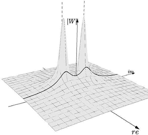
FIGURE 20.23
The module of the transfer function for the tank–pump system controlled in feedback highlighting its values along the imaginary axis.
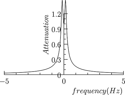
FIGURE 20.24
The Fourier representation of the tank–pump transfer function.
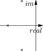
FIGURE 20.25
The poles of a Butterworth filter of the third-order.
An analog Butterworth filter can be implemented by an electronic circuit, as shown in in Figure 20.28. We are, however, interested here in its digital implementation, which can be carried out using the technique introduces in the previous section, that is
Find an appropriate value of the sampling period T.
Transform the transfer function W (s) expressed in the Laplace domain into the corresponding transfer function W (z) expressed in the Z domain by replacing s with (1 − z−1)/T, or using the bilinear transform s = 2(1 − z−1)/T (1 + z−1).
Implement the transfer function as a linear combination of previous samples of the input and of the output and the current input.
Up to now we have used informal arguments for the selection of the most appropriate value of the sampling period T. We have now the necessary background for a more rigorous approach in choosing the sampling period T.
20.2.3 The Choice of the Sampling Period
In the last section, discussing the choice of the sampling period T for taking signal samples and using them in the digital controller, we have expressed the informal argument that the value of T should be short enough to avoid losing significant information for that signal. We are now able to provide a more precise statement of this: We shall say that the choice of the sampling period T must be such that the continuous signal y(t) can be fully reconstructed from
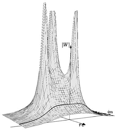
FIGURE 20.26
The module of a Butterworth filter of the third-order, and the corresponding values along the imaginary axis.
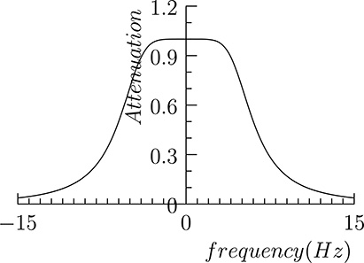
FIGURE 20.27
The module of the Fourier transform of a third-order Butterworth filter with 5 Hz cutoff frequency.
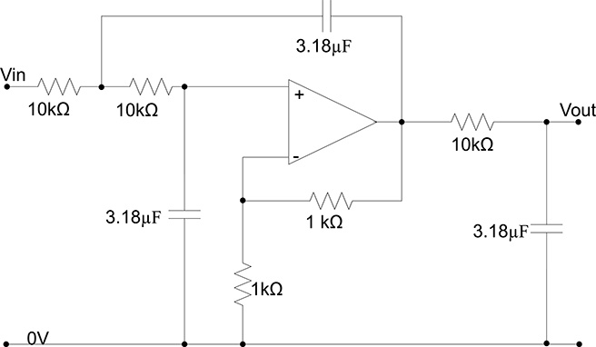
FIGURE 20.28
An electronic implementation of a Butterworth filter of the third order with 5 Hz cutoff frequency.
its samples y(nT ). Stated in other words, if we are able to find a mathematical transformation that, starting from the sampled values y(nT ) can rebuild y(t), for every time t, then we can ensure that no information has been lost when sampling the signal. To this purpose, let us recall the expression of the Fourier transform for the signal y(t)
Y(f)=∫∞-∞y(t)e-2Πftdt(20.75)(20.75)
which transforms the real function of real variable y(t) into a complex function of real variable Y (f ). Y (f ) maintains all the information of y(t), and, in fact, the latter can be obtained from Y (f ) via a the Fourier antitransform:
y(t)=∫∞-∞Y(f)ej2Πftdf(20.76)(20.76)
Now, suppose we have in hand only the sampled values of y(t), that is, y(nT ) for a given value of the sampling period T. An approximation of the Fourier transform can be obtained by replacing the integral in (20.75) with the summation
YT(f)=T∞∑n=-∞y(nT)e-j2ΠfnT(20.77)(20.77)
(20.77) is a representation of the discrete-time Fourier transform. >From YT (f ) it is possible to rebuild the original values of y(nT ) using the inverse transform
y(nT)=∫T/2-T/2YT(f)ej2ΠfnTdf(20.78)(20.78)
Even if from the discrete-time Fourier transform we can rebuild the sampled values y(nT ), we cannot yet state anything about the values of y(t) at the remaining times. The following relation between the continuous Fourier transform Y (f ) of (20.75) and the discrete time version YT (f ) of (20.77) will allow us to derive information on y(t) also for the times between consecutive samples:
yT(f)=1T∞∑r=-∞Y(f-rT)(20.79)(20.79)
Put in words, (20.79) states that the discrete time Fourier representation YT (f ) can be obtained by considering infinite terms, being the rth term composed of the continuous Fourier transform shifted on the right of rfc = r/T. The higher the sampling frequency fc, the more separate will be the terms of the summation. In particular, suppose that Y (f ) = 0 for |f | < f1 < fc/2. Its module will be represented by a curve similar to that shown in Figure 20.29. Therefore the module of the discrete time Fourier will be of the form shown in Figure 20.30, and therefore, for −fc/2 < f < fc/2, the discrete time transform YT (f ) will be exactly the same as the continuous one Y (f ).
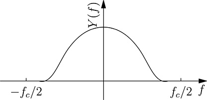
FIGURE 20.29
A frequency spectrum limited to fc/2.
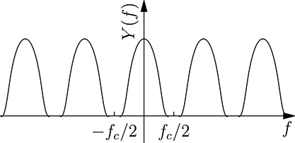
FIGURE 20.30
The discrete time Fourier transform corresponding to the continuous one of Figure 20.29.
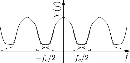
FIGURE 20.31
The Aliasing effect.
This means that, if the sampling frequency is at least twice the highest frequency of the harmonics composing the original signal, no information is lost in sampling. In fact, in principle, the original signal y(t) could be derived by antitrasforming using (20.76), the discrete-time Fourier transform, built considering only the sampled values y(nT ). Of course, we are not interested in the actual computation of (20.76), but this theoretical result gives us a clear indication in the choice of the sampling period T.
This is a fundamental result in the field of signal processing, and is called the Nyquist–Shannon sampling theorem, after Harry Nyquist and Claude Shannon, even if other authors independently discovered and proved part of it. The proof by Shannon was published in 1949 [80] and is based on an earlier work by Nyquist [67].
Unfortunately, things are not so bright in real life, and normally, it is not possible for a given function y(t) to find a frequency f0 for which Y (f ) = 0, |f | > f0. In this case we will have an aliasing phenomenon, as illustrated in Figure 20.31, which shows how the spectrum is distorted as a consequence of sampling. The effect of the aliasing when considering the sampled values y(nT ) is the “creation” of new harmonics that do not exists in the original continuous signal y(t). The aliasing effect is negligible for sampling frequencies large enough, and so the amplitude of the tail in the spectrum above fc/2 becomes small, but significant distortion in the sampled signal may occur for a poor choice of fc.
The theory presented so far provides us the “golden rule” of data acquisition,whensignalssampledby ADC convertersare thenacquired inanembedded system, that is, choosing a sampling frequency which is at least twice the maximum frequency of any significant harmonic of the acquired signal. However, ADC converters cannot provide an arbitrarily high sampling frequency, and in any case, this may be limited by the overall system architecture. As an example, consider an embedded system that acquires 100 signals coming from sensors in a controlled industrial plant, and suppose that a serial link connects the ADC converters and the computer. Even if the single converter may be able to acquire the signal at, say, 1 kHz (commercial ADC converters can have a sampling frequency up to some MHz), sending 100 signals over a serial link means that a data throughput of 100 KSamples/s has to be sustained by the communication link, as well as properly handled by the computer. Moving to a sampling frequency of 10 kHz may be not feasible for such a system because either the data link is not able to sustain an higher data throughput, or the processing power of the computer becomes insufficient.
Once a sampling frequency fc has been chosen, it is mandatory to make sure that the conversion does not introduce aliasing, and therefore it is necessary to filter the input signals with an analog low-pass filter whose cut-off frequency is at least fc/2, before ADC conversion. Butterworth filters, whose electrical schema is shown in Figure 20.28, are often used in practice, and are normally implemented inside the ADC boards themselves.
20.2.4 Building the Digital Low-Pass Filter
We are now ready to implement the digital low-pass filter with a cut-off frequency of 5 Hz similar to that which has been used to filter the signal shown in Figure 20.16, but using, for simplicity, 3 poles instead of 10 (used to obtain the filtered signal of Figure 20.18). We suppose a sampling frequency of 1 kHz, that is, T = 10−3s, assuming therefore that the spectrum of the incoming analog signal is negligible above 500 Hz.
Using (20.74), we obtain the following values for the three poles:
p1=(-15.7080+j27.2070)(20.80)(20.80)
p2=(-31.4159+j0)(20.81)(20.81)
p3=(-15.7080-j27.2067)(20.82)(20.82)
and, from (20.73), we derive the transfer function in the Laplace domain
W(s)=31006.28(s-(-15.708+j27.207))(s-(-31.416+j0))(s-(-15.708-j27.207))(20.83)(20.83)
From the above transfer function, with the replacement s = (1 − z−1)/T, T = 10−3, we derive the transfer function in the Z domain
W(z)=3.1416×10⁻⁵-z-3+3.0628z-2-3.1276z-1+1.06483(20.84)(20.84)
and finally the actual computation for the desired low-pass digital filter:
y((n-3)T)-3.063y((n-2)T)+3.⋅128y((n-1)T)+3.142×10⁻⁵x(nT)1065(20.85)(20.85)
We recognize that, in the general case, the implementation of a low-pass filter (and more in general of the discrete time implementation of a linear system) consists of a linear combination of the current input, its past samples and the past samples of the output. It is therefore necessary to keep in memory the past samples of the input and output. A common technique that is used in order to avoid unnecessary copies in memory and therefore minimize the execution time of digital filters is the usage of circular buffers. A circular buffer is a data structure that maintains the recent history of the input or output. When new samples arrive, instead of moving all the previous samples in the buffer array, the pointer to the head of the buffer is advanced instead. Then, when the head pointer reaches one end of the history array, it is moved to the other end: If the array is large enough to contain the required history the samples on the other end of the array are no more useful and can be discarded. Below is the C code of a general filter implementation. Routine initFilter() will build the required data structure and will return a pointer to be used in the subsequent call to routine doFilter(). No memory allocation is performed by routine doFilter(), which basically performs a fixed number of sums, multiplications and memory access. In fact, this routine is to be called run time, and for this reason it is important that the amount of time required for the filter computation is bounded. Conversely, routine initFilter() has to be called during system initialization since its execution time may be not predictable due to the calls to system routines for the dynamic memory allocation. An alternative implementation would have used statically allocated buffers and coefficient array, but would have been less flexible. In fact, the presented implementation allows the run-time implementation of a number of independent filters.
/*   Filter Descriptor Structure : fully describes the filter and
     its current state.
     This structure contains the two circular buffers and the
     current index within them.
     It contains also the coefficients  for the previous input
     and output samples for the  filter computation
     y(nT) = aN*y((n–N)T)+...+a1*y((n–1)T)
        + bMu((n-M)T)+...+b1*u((n–1)T + b0*u(nT) */
typedef struct     {
    int   currIndex;         //Current index in circular buffers
    int  bufSize ;   //Number of elements in the buffers
    float  * yBuf ;  //Output history buffer
    float  * uBuf ;  //Input history buffer
    float  *a;             //Previous output coefficients
    int  aSize ;           //Number of a coefficient
    float  *b;             //Previous input coefficients
    int  bSize ;           //Number of b coefficients
} FilterDescriptor;
/*   Filter structure initialization .
     To be called before entering the real–time phase
     Its arguments are the a and b coefficients of the filter  */
FilterDescriptor * initFilter( float *aCoeff, int numACoeff ,
    float * bCoeff, int  numBCoeff)
{
    int i;
    FilterDescriptor * newFilter;
    newFilter = ( FilterDescriptor *) malloc ( sizeof ( FilterDescriptor));
/* Allocate and copy filter  coefficients  */
    newFilter ->a = ( float *) malloc ( numACoeff   * sizeof ( float ));
    for(i = 0; i < numACoeff; i ++)
    newFilter ->a[i]  =  aCoeff [i];
    newFilter -> aSize  = numACoeff;
    newFilter ->b = ( float *) malloc ( numBCoeff   * sizeof ( float ));
    for(i = 0; i < numBCoeff; i ++)
       newFilter ->b[i]  =  bCoeff [i ];
    newFilter -> bSize  = numBCoeff;
/*   Circular Buffer dimension is the greatest between the number
     of a and b coefficients  */
    if( numACoeff >   numBCoeff)
      newFilter -> bufSize  =  numACoeff;
    else
      newFilter -> bufSize  =  numBCoeff;
/*   Allocate circularBuffers,  initialized to 0  */
    newFilter -> yBuf = ( float *) calloc ( newFilter -> bufSize,  sizeof ( float ));
    newFilter -> uBuf = ( float *) calloc ( newFilter -> bufSize,  sizeof ( float ));
/*   Buffer index starts at 0 */
    newFilter -> currIndex =  0;
    return  newFilter;
}
/*   Run time filter computation .
     The first argument is a pointer to the filter descriptor
     The second argument is the current input
     It returns the current output  */
float doFilter ( FilterDescriptor *filter, float       currIn )
{
    float currOut =  0;
    int i;
    int currIdx ;
/*  Computation of the current output based on previous input
    and output  history  */
    currIdx = filter -> currIndex;
    for(i = 0; i < filter -> aSize ;   i++)
    {
     currOut += filter ->a[i]*    filter -> yBuf [currIdx ];
/*  Go to previous sample in the circular        buffer  */
      currIdx --;
      if( currIdx <  0)
        currIdx +=   filter -> bufSize ;
    }
    currIdx = filter -> currIndex;
    for(i = 0; i < filter -> bSize -1; i++)
    {
      currOut += filter ->b[i +1]* filter -> uBuf[ currIdx ];
/*  Go to previous sample in the circular        buffer  */
      currIdx --;
      if( currIdx <  0)
        currIdx +=   filter -> bufSize ;
    }
/*   b [ 0 ] contains the coefficient  for the current      input */
    currOut +=  filter ->b [0]* currIn ;
/*   Upate input and output  filters */
    currIdx = filter -> currIndex;
    currIdx ++;
    if( currIdx == filter -> bufSize )
      currIdx = 0;
    filter -> yBuf [ currIdx ] = currOut ;
    filter -> uBuf [ currIdx ] =  currIn ;
    filter -> currIndex  = currIdx ;
    return currOut ;
}
/*   Filter deallocation  routine .
     To be called when the filter  is no longer used outside
     the real-time phase  */
void  releaseFilter( FilterDescriptor * filter )
{
    free (( char  *) filter ->a);
    free (( char  *) filter ->b);
    free (( char  *) filter -> yBuf );
    free (( char  *) filter -> uBuf );
    free (( char *) filter );
}
20.2.5 Signal to Noise Ratio (SNR)
Up to now we have seen the main components of a digital low-pass filter, that is, antialiasing analog filtering, data sampling and filter computation. The resulting data stream can be used for further computation or converted to an analog signal using a DAC converter if filtering is the only function of the embedded system. We have seen how information may be lost when sampling a signal, and the techniques to reduce this effect. There is, however, another possible reason for information loss in the above chain. The ADC converter, in fact, converts the analog value of the input into its digital representation using a finite number of bits. This unavoidably introduces an error calledthe quantization error. Its effect can be considered as a superimposed noise in the input signal. If N bits are used for the conversion, and A is the input range for the ADC converter, the quantization interval is Δ = A/2N, and therefore, the quantization error e(nT ) is included in the interval [−Δ/2, Δ/2]. The sequence e(nT ) is therefore a sequence of random values, which is often assumed to be a strictly stationary process, where the probability distribution of the random samples is not related to the original signal y(nT ). It does not change over time, and the distribution is uniform in the interval [−Δ/2, Δ/2]. Under these assumptions, the probability distribution of the error is
fe(a)=1Δ,-Δ2≤a≤Δ2(20.86)(20.86)
For such a random variable e, its power, that is, the expected value E[e2] is
Pe=E[e2]=∫∞-∞a2fe(a)da=∫Δ/2-Δ/2a2ΔΔ212(20.87)(20.87)
An important parameter in the choice of the ADC device is the signal-to-noise ratio (SNR), which expresses the power ratio between the input signal and its noise after sampling, that is,
SNR=10log10PsignalPnoise(20.88)(20.88)
using the expression of the power for the quantization error (20.87), we have
SNR=10log10PsignalPnoise=10log10-10log10Δ212(20.89)(20.89)
If we use B bits for the conversion, and input range of A, the quantization interval Δ is equal to A/(2B) and therefore
SNR=10log10Psignal+10log1012-20log10A+20Blog102=CONST+6.02B(20.90)(20.90)
that is, for every additional bit in the conversion, the SNR is incremented of around 6dB for every additional bit in the ADC conversion (the other terms in (20.90) are constant). This gives us an estimation of the effect of the introduced quantization error and also an indication on the number of bits to be considered in the ADC conversion. Nowadays, commercial ADC converters use 16 bits or more in conversion, and the number of bits may reduced for very high-speed converters.
20.3 Summary
In this section we have learned the basic concepts of control theory and the techniques that are necessary to design and implement a digital low-pass filter. The presented concepts represent facts that every developer of embedded systems should be aware of. In particular, the effects of sampling and the consequent harmonic distortion due to the aliasing effect must always be taken into account when developing embedded systems for control and data acquisition. Another important aspect that should always be taken in consideration when developing systems handling acquired data, is the choice of the appropriate number of bits in analog-to-digital conversion. Finally, once the parameters of the linear system have been defined, an accurate implementation of the algorithm is necessary in order to ensure that the system will have a deterministic execution time, less than a given maximum time. Most of this book will be devoted to techniques that can ensure real-time system responsiveness. A precondition to every technique is that the number of machine instructions required for the execution of the algorithms is bounded. For this reason, in the presented example, the implementation of the filter has been split into two sets of routine: offline routines for the creation and the deallocation of the required data structures, and an online routine for the actual run-time filter computation. Only the latter one will be executed under real-time constraints, and will consist of a fixed number of machine instructions.