The aspect that we have neglected so far is that many systems do not respond immediately to a control input; instead, they respond with some form of lag or delay. In addition, many systems exhibit even more complicated behavior when stimulated. These factors need to be taken into account when designing a control loop.

Let’s consider a few examples (see Figure 3-1 and Figure 3-2).

Of course, all of these behaviors can also occur in combination.

Transient Response and Steady-State Response

The response of a system to an external disturbance often consists of both a transient component, which disappears over time, and a steady-state component. These components are well illustrated by the spring–mass system: the initial oscillations die away in time, so they are transient. But the overall displacement of the mass, which is the result of the change in position of the spring’s free end, persists in the steady state.

Figure 3-1. Examples of dynamical systems and their response to an external stimulus. These types of behavior are common among industrial processes and computer systems.

Control actions are often applied to bring about a change in the steady-state output. (If you turn up the heat, you want the room to be warmer and to stay that way.) From this perspective, transient responses are viewed mainly as a nuisance: unwanted accompaniments of an applied change. Hence an important measure for the performance of a control system is the time it takes for all transient components of the response to have disappeared. Usually, handling the transient response in a control system involves an engineering trade-off: systems in which transients are strongly damped (so that they disappear quickly) will respond more slowly to control inputs than do systems in which transient behavior is suppressed less strongly.

Figure 3-2. Additional examples of dynamical systems and their response to an external stimulus. The oscillatory response is especially important among mechanical and electrical systems. The initial response in the direction opposite to the external influence makes non-minimum phase systems difficult to control.

All objects in the physical world exhibit some form of lag or delay, and most mechanical or electrical systems will also have a tendency to oscillate.

The reason for the lags or delays is that the world is (to use the proper mathematical term) continuous: An object that is in some place now cannot be at some totally different place a moment later. The object has to move, continuously, from its initial to its final position. It can’t move infinitely quickly, either. Moreover, to move a physical object very quickly requires large amounts of force, energy, and power (in the physical sense), which may not be available or may even be impossible to supply. (Accelerating a car from 0 to 100 km/h in 5 seconds takes a large engine, to do so in 0.5 seconds would take a significantly larger engine, and a very different mode of propulsion, too.) The amount by which objects in the physical world can move (or change their state in any other way) is limited by the laws of nature. These laws rule supreme: No amount of technical trickery can circumvent them.

For computer systems, however, these limitations do not necessarily apply in quite this way! A computer program can arbitrarily change its internal state. If I want to adjust the cache size from 10 items to 10 billion items, there is nothing to stop me—the next time through the loop, the cache will have the new size. (The cache size may be limited by the amount of memory available, but that is not a fundamental limitation—you can always buy some more.) In particular, computer programs do not exhibit the partial response that is typical of continuous systems. You will typically get the entire response at once. If you asked for a 100-item cache, you will get the entire lot the next time through the loop—not one item now, five more the next time around, another 20 coming later, and so on. In other words, computer programs typically do not exhibit lags. They do, however, exhibit delays; these are referred to as “latency” in computer terminology. If you are asking for 20 additional server instances in your cloud data center, it will take a few minutes to spin them up. During that time, they are not available to handle requests—not even partially. But once online, they are immediately fully operational. Figure 3-3 shows schematically the typical response characteristic of a computer program. Compared to the “smooth” behavior of physical objects displayed in Figure 3-1 and Figure 3-2, the dynamics of computer applications tend to be discontinuous and “hard.”

Figure 3-3. Typical dynamical response of a computer system: The response is discontinuous and occurs after a measurable delay.

The considerations of the preceding paragraph apply to standalone computer applications. For computer systems, which consist of multiple computers (or computer programs) communicating with each other and perhaps with the rest of the world (including human users), things are not quite as clear-cut. For instance, recall our example of the item cache. We can adjust the size of the cache from one iteration to the next, and by an arbitrary amount. But it does not follow that the hit rate (the tracked quantity or “output” for this system) will respond just as quickly. To the contrary, the hit rate will show a relatively smooth, lag-type response. The reason is that it takes time for the cache to load, which slows the response down. Moreover, the hit rate itself is necessarily calculated as some form of trailing average over recent requests, so some time must elapse before the new cache size makes itself felt. In the case of the additional server instances being brought up in the data center, we may find that not all the requested instances come online at precisely the same moment but instead one after another. This also will tend to “round out” the observed response.

Another case of computer systems exhibiting nontrivial dynamics consists of systems that already include a “controller” (or control algorithm) of some form. For example, it is common practice to double the size of a buffer whenever one runs out of space. Similar strategies can be found, for instance, in network protocols, for the purpose of maximizing throughput without causing congestion. In these and similar situations, the behavior of the computer system is constrained by its own internal control algorithms and will not change in arbitrary ways.

The reason we spend so much time discussing these topics is that lags and delays make it much more difficult to design a control system that is both stable and performant. Take the heated vessel: Initially, we want to raise its temperature and so we apply some heat. When we check the output a short while later, we find that the temperature has barely moved (because it’s lagging behind). If we now increase the heat input, then we will end up overheating the vessel. To avoid this outcome, we must take the presence (and length) of the lag into account.

Moreover, unless we are careful we might find ourselves applying corrective action at precisely the wrong moment: Applying a control action intended to reduce the output precisely when the output has already begun to diminish (but before this is apparent in the actual system output). If we reach this scenario, then the closed-loop system undergoes sustained oscillations. (Toward the end of this chapter, you will find a brief computer exercise that demonstrates how the delay of even a single step can lead to precisely this situation.)

There exists a very well-developed, beautiful, and rather deep theory to describe the dynamic behavior of feedback loops, which we will sketch in Part IV. An essential ingredient of this theory is knowledge of the dynamic behavior of the controlled system. If we can describe how the controlled system behaves by itself, then the theory helps us understand how it will behave as part of a feedback loop. In particular, the theory is useful for understanding and calculating the three essential properties of a feedback system (stability, performance, and accuracy) even in the presence of lags and delays.

The theory does require a reasonably accurate description of the dynamics of the system that we wish to control. For many systems in the physical world, such descriptions are available in the form of differential equations. In particular, simple equations describing mechanical, electrical, and thermal systems are well known (the so-called laws of nature), and the entire theory of feedback systems was really conceived with them in mind.

For computer systems, this is not the case. There are no laws, outside the program itself, that govern the behavior of a computer program. For entire computer systems there may be applicable laws, but they are neither simple nor universal; furthermore, these laws are not known with anything like the degree of certainty that applies to, say, a mechanical assembly. For instance, one can (at least in principle) use methods from the theory of stochastic processes to work out how long it will take for a cache to repopulate after it has been resized. But such results are difficult to obtain, are likely to be only approximate, and in any case depend critically on the nature of the traffic—which itself is probably not known precisely.

This does not mean that feedback methods are not applicable to computer systems—they are! But it does mean that the existing theory is less easily applied and provides less help and insight than one might wish. Developing an equivalent body of theoretical understanding for computer systems and their dynamics is a research job for the future.

To understand how even a simple delay can give rise to nontrivial behavior when encountered in a feedback architecture, let’s consider a system that simply replicates the input from the previous time step to its output. We close the feedback loop as in Figure 2-1 and use a controller, which merely multiplies its input by some constant k.

The brief listing that follows shows a program that can be used to experiment with this closed-loop system. The program reads both the setpoint r and the controller gain k from the command line. The iteration itself is simple: The tracking error and the controller output are calculated as in Chapter 2, but the current output y is set to the value of the controller output from the previous time step. Figure 3-4 shows the time evolution of the output y for two different values of the controller gain k.

import sys

r = float(sys.argv[1]) # Reference or "setpoint"
k = float(sys.argv[2]) # Controller gain

u = 0        # "Previous" output
for _ in range( 200 ):
    y = u        # One-step delay: previous output

    e = r - y    # Tracking error
    u = k*e      # Controller output

    print r, e, 0, u, y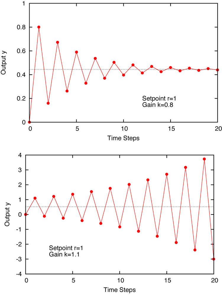

Figure 3-4. Time evolution of the system y_t+1 = k(r – y_t) for two different values of k.

Although the setpoint is constant, the process output oscillates. Moreover, for values of the controller gain k greater than 1, the amplitude of the oscillation grows without bounds: The system diverges.

If you look closely, you will also find that the value to which the system converges (if it does converge) is not equal to the desired setpoint. (You might want to base control actions on the cumulative error, as in Chapter 2. Does this improve the behavior?)