We want to control the speed of cooling fans to maintain a desired temperature of the cooled component. The control output is the temperature, the control input is the fan speed, which is adjustable continuously so that we can treat it as a floating-point number. The heat generated by the CPU depends on its “load,” which we will model as changing by fixed steps at random intervals. We will also assume that the ambient temperature may undergo slow, random drifts. Besides these two effects, the system is essentially deterministic.

As mentioned in Chapter 5, the dynamics we wish to control are the cooling dynamics—that is, the reduction in temperature as the fan speed is increased. The initial state, where the system is considered to be “off,” therefore corresponds to the situation with minimal cooling (with the fan speed reduced to the lowest possible speed that won’t damage the CPU). This initial state does not correspond to the situation where the CPU is itself switched off, as we are not concerned about the dynamics of the CPU heating up after first being powered on.

The temperature of a body losing heat to the environment is described by Newton’s law of cooling, . Here Θ is the temperature difference between the body and its environment:^[18]

and u describes any heat supplied to the body from outside “sources.”

To understand what this differential equation tells us, it is convenient to rewrite it in the following form:

The change in temperature (per unit of time) consists of two contributions, a loss of temperature and a gain of cu. Let’s first consider the case where no heat is supplied: u = 0. A cup of coffee cooling on the desk is an example. In this situation, the body loses a certain fraction of its temperature every moment. The parameter T is the time scale of the problem: the length of time it takes for the temperature to drop to about one-third of its original value.

The other term on the right-hand side describes any heat supplied to the body. In the CPU example, this is the heat generated by the chip as it is operating. The quantity u is the flow of heat to the body, measured in joules per second (or watts). As the load on the processor changes, so will the amount of heat u generated. The coefficient c describes by how many degrees the body heats up for each joule of energy supplied (basically, c is the heat capacity of the body). You can convince yourself that cu has the dimension of temperature/time.

But where is our fan speed? It is there, hiding inside the quantity T: if the fan runs faster, then the processor will take less time to shed the same amount of heat and so T will be smaller. The way the control action enters the equation is a bit sneaky: usually, the control action would be a linear term on the right-hand side, like u. (In fact, the same equation describes a pot that is heated, in which case the control action u is the supplied heat.)

We can now collect all the pieces. If initially the body is at temperature Θ(t), then its temperature a short time δt later is

Here we have made use of the fact that the derivative can be approximated as a finite difference:

This approximation is good provided that δt is sufficiently small—in other words, as long as Θ does not change much during an interval of duration δt. For us, this means that δt must be much smaller than T (since T is the time scale over which Θ changes significantly).

As long as T and u are held constant, we can find an explicit solution to the differential equation. Under the stated conditions, the temperature at time t is given by

where the constant Θ₀ is determined by the initial temperature. For instance, if the initial temperature is zero (Θ(0) = 0) then Θ₀ must be –cuT. This describes the situation when the computer is initially switched off and is being turned on at t = 0. (Remember that Θ is the temperature above the ambient one.)

Finally, we need to find numerical values for the various parameters. The power consumption of a current processor is about 75 watts, and I will assume that the power can change in steps of 10 watts as the load changes. The parameters T and c must, in principle, be measured. Here, I estimate T = 120 seconds. That is to say: without the fans running, the processor will drop from 200 degree Celsius to about 70 degree Celsius within 2 minutes; it will cool down faster with the fans running. We can then find c from the final, steady-state temperature that the processor reaches without active cooling. In this limit, Θ(∞) = cuT. Assuming that the maximum temperature is 200 degrees Celsius, and plugging in our estimates for u and T, we find degrees Celsius per joule.

Figure 17-1 shows the kinds of measurements we would perform to determine the values of the parameters.^[19] The graph includes curves for several different types of open-loop measurement. One curve shows the temperature development for the CPU without any of the fans running. The temperature tops out somewhere near 200 degrees, at which point the chip has overheated and serves only as a space heater but is useless for any other purpose!

Figure 17-1. Time development of the CPU temperature in an open-loop arrangement. The fan speed is suddenly increased from its minimal setting to various higher speeds at t = 5 minutes, resulting in greater cooling action and a decrease in temperature (step test).

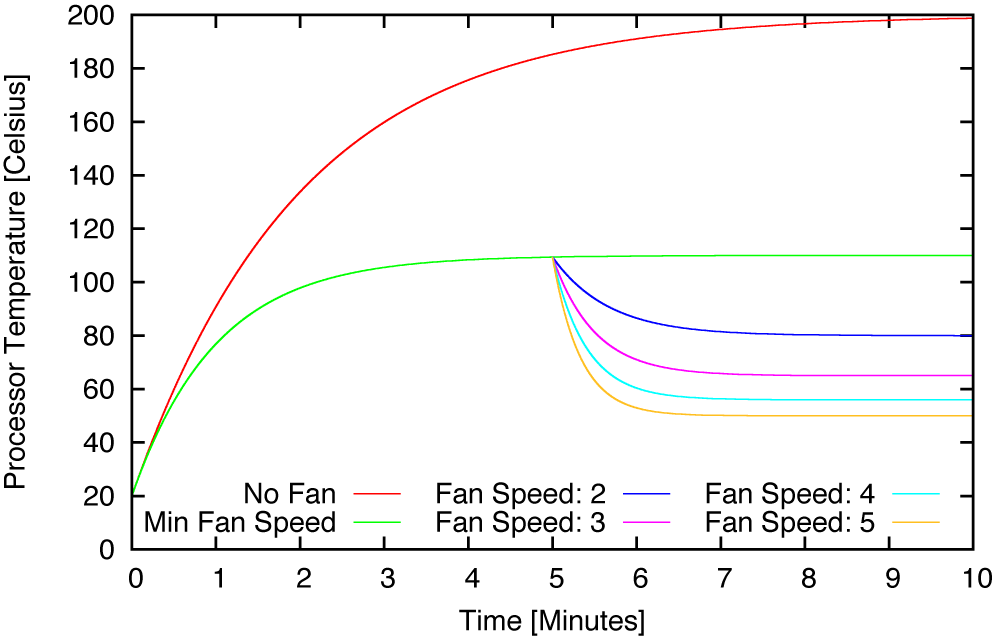
Let’s suppose the maximal operating temperature that won’t damage the chip is 100 degrees. Maintaining this temperature requires the fans to be running, but at minimum speed. At t = 5 minutes, we increase the fan speed: that’s basically the kind of “step test” discussed in Chapter 8, and from the graph we can read off the decrease in temperature due to this control action. (Note that the decrease in temperature is not a linear function of the fan speed.)

The figure shows that the delay τ is negligible and that the time constant T is approximately 1 minute (60 seconds). At fan speed 4, the temperature reduction is about 40 degrees and so the static gain factor Δ u/Δ y is approximately 4/40 = 0.1. Quite satisfactory closed-loop performance is found with k_p = 2.0 and k_i = 0.5.

In Figure 17-2 we see how this system behaves in production. The set-point is initially set to 50 degrees and is later reduced to 45 degrees. The load on the processor keeps changing, and with it the amount of heat generated. But whenever the amount of heat increases, the fan speed increases with it to keep the CPU temperature at the setpoint. The temperature overshoots a little whenever the load level changes, but it quickly reaches the desired setpoint again.

Figure 17-2. Time development of the CPU temperature under closed-loop control. The fan is not capable of delivering the required cooling actions if the CPU is working under maximum load (actuator saturation, t = 11, ..., 14).

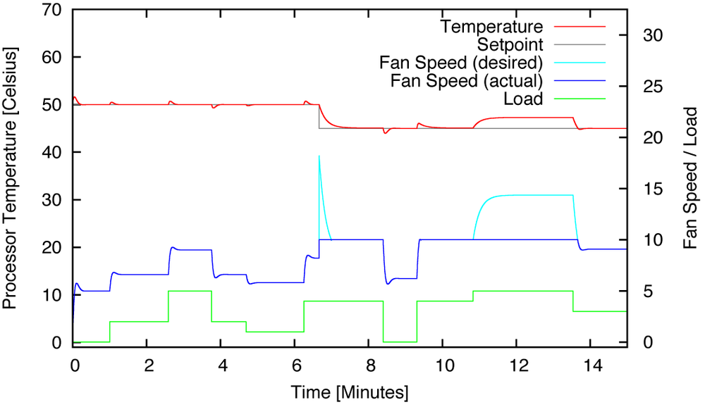
One practical problem exhibited by the system is the occurrence of actuator saturation. The fans are not capable of keeping the CPU at 45 degrees at the highest load level, with the consequence that the desired fan speed (as calculated by the controller) is higher than the actual speed that the fan can achieve. It is therefore important to use a “clamping” controller, which stops adding to the integral term once the actuator is maxed out (see Chapter 10).

The dynamics of the system in the present case study are described by a differential equation; simulating it therefore means solving (or “integrating”) this differential equation. In the code that follows, this is done in the simplest possible manner. We take the equation in the form

and translate it directly into code. This equation amounts to an updating algorithm for Θ(t): it uses the temperature at time t to calculate the temperature at a later time t + δt. The quantity T, which describes how quickly the CPU cools down, is a combination of the natural heat loss and the heat loss due to active cooling from the fan. The term u(t), which describes the heat generated by the CPU, is a combination of the chip’s idle power and the additional heat if the CPU is running under increased load. The load itself changes at random times by a fixed amount.

import random
import feedback as fb

class CpuWithCooler( fb.Component ):
    def __init__( self, jumps=False, drift=False ):
        self.ambient = 20             # temperature: degree C
        self.temp    = self.ambient   # initial temperature

        self.wattage = 75             # CPU heat output: J/sec
        self.specific_heat = 1.0/50.0 # specific heat: degree/J

        self.loss_factor = 1.0/120.0  # per second

        self.load_wattage_factor = 10 # addtl watts due to load
        self.load_change_seconds = 50 # avg sec between changes
        self.current_load = 0

        self.ambient_drift = 1.0/3600 # degrees per second

        self.jumps = jumps            # jumps in CPU load?
        self.drift = drift            # drift in ambient temp?


    def work( self, u ):
        u = max( 0, min( u, 10 ) )      # actuator saturation

        self._ambient_drift()           # drift in ambient temp
        self._load_changes()            # load changes, if any

        diff = self.temp - self.ambient # temperature diff
        loss = self.loss_factor*(1 + u) # natural heatloss+fan

        flow = self.wattage + self.current_load # CPU heat flow

        self.temp += fb.DT*(self.specific_heat*flow - loss*diff)
        return self.temp


    def _load_changes( self ):
        if self.jumps == False: return

        s = self.load_change_seconds
        if random.randint( 0, 2*s/fb.DT ) == 0:
            r = random.randint( 0, 5 )
            self.current_load = self.load_wattage_factor*r

    def _ambient_drift( self ):
        if self.drift == False: return

        d = self.ambient_drift
        self.ambient += fb.DT*random.gauss( 0, d )
        self.ambient = max( 0, min( self.ambient, 40 ) )


    def monitoring( self ):
        return "%f" % ( self.current_load, )

The units we use in this case study to measure wall-clock time are seconds, and all other units are compatible with this scale (for example, watts equal joules per second). As we saw previously, the typical time scale on which the system’s temperature changes significantly is about 1 minute. We therefore need to take steps that are at least one order of magnitude smaller than that—about a second or less. In the end, I used steps of one-hundredth of a second (fb.DT = 0.01) for extra accuracy, although one-tenth of a second (fb.DT = 0.1) would have been sufficient.

One important aspect that this example aims to demonstrate is the effect of actuator saturation: there is a maximum cooling effect the fan can achieve, because at some point it simply can’t run any faster. The output of the fan is even more constrained in the opposite direction, because the fan output can never become negative (corresponding to a heating effect).

To model this behavior, a Limiter element has been included in the position of an actuator between the controller and the plant. This element constrains its output to the range that was specified when the element was first created, and any input that exceeds this range is trimmed to the most extreme value still within the permitted range.

class Limiter( fb.Component ):
    def __init__( self, lo, hi ):
        self.lo = lo
        self.hi = hi

    def work( self, x ):
        return max( self.lo, min( x, self.hi ) )

Given the effect of this Limiter, it is important to use a clamping controller. So instead of the simple PidController, we use an AdvController instance, where the clamping range is set equal to the range permitted by the actuator.

fb.DT = 0.01

def setpoint(t):
    if t < 40000: return 50
    else: return 45

p = CpuWithCooler( True, True ); p.temp = 50 # Initial temp
c = fb.AdvController( 2, 0.5, 0, clamp=(0,10) )

fb.closed_loop( setpoint, c, p, 100000, inverted=True,
                actuator=fb.Limiter( 0, 10 ) )