
Chapter 5. Identifying Input and Output Signals
Initially, it can be difficult to see how feedback methods can be applied to situations other than the “classical” application areas treated in textbooks on control theory. The way control engineering decomposes real-world systems into abstractions often does not easily align with the way those systems appear to others. In this chapter, I want to step through a handful of examples and show how they could be approached from a control-theoretic point of view.
Control Input and Output
The essential abstraction in any control problem is the plant or process: the system that is to be controlled. From a controls perspective, a plant or process is a black box that transforms an input to an output. It is usually not difficult to recognize the plant itself, but identifying what to use as control input and output can be challenging.
It is essential to realize that the terms “input” and “output” here are used only in relation to the control problem and may be quite different from the functional inputs and outputs of the controlled system. Specifically:
These two observations should help to identify the quantities to use as control signals, either as input or as output. Just ask yourself:
What quantity can we influence directly?
What quantity do we (ultimately) want to influence?
In books on control theory, the output is often referred to as the “process variable” (PV) and the input as the “control variable” or “manipulated variable” (MV). Both taken together define the system’s “interface” (in a software-engineering sense of the word).
There may be situations where both of these quantities are identical. In this case, you are done and you can stop reading. But often they will not be the same—and then you have a control problem.
Directionality of the Input/Output Relation
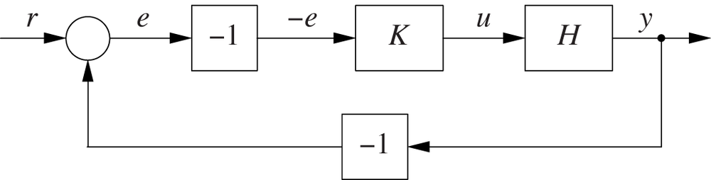
The basic idea of feedback control is to compare the actual plant output y to the reference value r and then to apply a corrective action that will reduce the tracking error e = r – y. In order to do so, we must know in which direction to apply the correction. Let’s say that the output y is smaller than what it should be (y < r), so that the tracking error is positive. Obviously, we want to increase the process output—but does this mean we need to increase the plant input u or decrease it?
The answer depends on the directionality of the input/output relation for the controlled system. It is usually assumed that increasing the control input will increase the control output:
Increasing the power supplied to a heating element (the input) will increase the temperature of the heated room or vessel (the output).
Increasing the number of servers in a data center will increase the number of requests handled per hour.
However, the opposite also occurs:
Increasing the power supplied to a cooling unit (the input) will decrease the temperature in the cooled room or vessel (the output).
Increasing the number of servers in a data center will reduce the average response time for server requests.
The directionality depends on the specific choice of input and output signals, not on the overall plant or process, as is demonstrated by the data center example. Depending on the particular choice of output signal, the same system can exhibit either form of directionality.
We need to take the input/output directionality into account when designing a control loop to ensure that corrective actions are applied in the appropriate direction. A standard loop (Figure 5-1) is suitable for the “normal” case, where an increase in control input results in an increase in control output. For the “inverse” case (where an increase in control input leads to a decrease in output), we can use a loop as in Figure 5-2. In this loop, the tracking error e is multiplied by −1 before being passed to the controller.[5]

Examples
Let’s consider a few examples and discuss the available options for both control inputs and outputs as well as their advantages and disadvantages. When evaluating each situation, we are primarily concerned with two properties: which signals are available and which signals will show the speediest response. (In Part III, we will study many of these examples in more depth.)
Thermal Control 1: Heating
Situation
A room is to be kept at a comfortable temperature, or a vessel containing some material is to be kept at a specific temperature.
Input
The input is the amount of heat applied; this may be the dial setting on the stove, the voltage applied to the heating element, or the flow of heating oil to the furnace.
Output
In any case, the temperature of the heated object is the output of the process.
Commentary
This example is a conventional control problem, where the control strategy—including the choice of input and output signals—is pretty clear. Notice that the control strategy can vary: central heating often has only an on/off controller, whereas stoves let you regulate their power continuously.
Although simple in principle, this example does serve to demonstrate some of the challenges of control engineering in the physical world. We said that the output of the plant is “the temperature” and that its input is “the heat supplied.” Both are physical quantities that are not easy to handle directly. Just imagine having to develop a physical device to use as a PID-controller that takes “a temperature” as input and produces a proportional amount of “heat” as output! For this reason, most control loops make use of electronic control signals. But this requires the introduction of additional elements into the control loop that can turn electric signals into physical action and observed quantities into electric signals (see Figure 5-3, top).
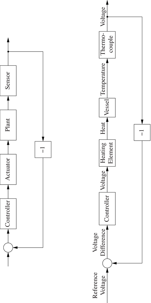
Elements that convert back and forth between control signals and physical quantities are generally known as transducers. A transducer that measures a physical quantity and turns it into a control signal is called a sensor, and a transducer that transforms a control signal into a physical control action is called an actuator. In the case of the heated vessel, the sensor might be a thermocouple (transforming a measured temperature into a voltage), and the actuator would be a heating element, transforming an applied voltage into heat (Figure 5-3, bottom). If the vessel to be heated is large (such as a reaction vessel in the chemical industry) or if high temperatures are required (as in a furnace), then a single actuator might not be enough; instead we might find additional power amplifiers between the controller and the actual heating element.
Transducers introduce additional complexity into the control loop, including nonlinearities and nontrivial dynamics. Sensors in particular may be slow to respond and may also be subject to measurement noise. (The latter might need to be smoothed using a filter, introducing additional lags.) Actuators, for their part, are subject to saturation, which occurs when they physically cannot “keep up” with the control signal. This happens when the control signal requires the actuator to produce a very large control action that the actuator is unable to deliver. Actuators are subject to physical constraints (there are limits on the amount of heat a heating element can produce per second and on the speed with which a motor can move, for example), limiting their ability to follow control signals that are too large.
In computer systems, transducers rarely appear as separate elements (we do not need a special sensor element to observe the amount of memory consumed, for instance), and—with the exception of actuator saturation—most of their associated difficulties do not arise. Actuator saturation, however, can be a serious concern even for purely virtual control loops. We will return to this topic in Chapter 10 and in the case studies in Part III.
Item Cache
Situation
Consider an item cache—for instance, a web server cache. If a request is made to the system, the system first looks in the cache for the requested item and returns it to the user if the item is found. Only if the item is not found will the item be retrieved from persistent storage. The cache can hold a finite number of items, so when an item is fetched from persistent storage, it replaces the oldest item currently in the cache. (We will discuss this system in detail as a case study in Chapter 13.)
Input
The quantity that can be controlled directly is the number of items in the cache.
Output
The quantity that we want to influence is the resulting “hit” or success rate. We desire that some fraction (such as 90 percent) of user requests can be completed without having to access the persistent storage mechanism.
Commentary
Observe that the quantities identified as “input” and “output” from a control perspective have nothing to do with the incoming user requests or the flow of items into and out of the cache. This is a good example of how the control inputs and outputs can be quite different from the functional inputs and outputs of a system—it is important not to confuse the two!
Also, the definition of the output signal is still rather vague. What does “90 percent hit rate” mean in practice? Ultimately, each hit either succeeds or fails: the outcome is binary. Apparently we need to average the results of the last n hits to arrive at a hit rate, which leads us to ask: how large should n be? If n is large, then the outcome will be less noisy but the memory of the process will be longer, so it will respond more slowly to changes (see Chapter 3). Selecting a specific value for n therefore involves a typical engineering trade-off.
We also need to define how the average is to be taken. Do we simply calculate a straight average over the last n requests? Or should we rather weight more recent requests more heavily than older requests? For practical implementations, it may be convenient to employ an exponential smoothing method (a recursive digital filter), where the value of the hit rate st at time t is calculated as a mixture of the outcome of the most recent user request σt and the previous value of the hit rate:

Here, σt is either 0 or 1, depending on the outcome of the most recent cache request. The smaller α is, the smoother the signal will be. (In fact, we can choose whether to consider the filter as part of the system itself or to treat it as a separate component. In the former case, the system output will be the smoothed hit rate; in the latter case, the system output will be the string of 0’s and 1’s corresponding to the outcome of the most recent request.)
Finally, we should discuss the notion of “time” t. From the preceding remarks it is clear that the system will not produce a new and different value of its output unless a user request is made. We must decide when control inputs (that is, changes to the size of the buffer) can be made: only synchronously with user requests, or asynchronously at any time that we desire (for instance, periodically once per second)? In the asynchronous case, the main “worker thread” of the cache (the one that handles user requests) will be separate from the “control thread” that handles control inputs. This is yet another reminder that control flow and functional flow are quite separate things.
Server Scaling
Situation
Imagine a central server performing some task. It could be a web server serving user requests, or a compute server performing CPU-intensive jobs, or even a DB server. In any case, we can control the number of active “worker” instances (the number of threads in the case of the web server, or the number of CPUs for the compute server, and so on). Incoming requests are assigned to the next available worker instance; it will take the worker some (random) amount of time to complete each request. Requests that cannot be served immediately are submitted to a queue. There is no guarantee that the throughput of the server will scale linearly with the number of active worker instances! (More specific systems fitting this general description will be discussed in detail in Chapter 15 and Chapter 16.)
Input
We can select the number of active worker instances directly.
Output
Ultimately, we want to make sure tasks are flowing through the system without being held up. However, we have a wide selection of metrics that can be used for that purpose. These include:
Number of requests queued (the queue length)
Net change in the length of the queue (over some time interval)
Average age of requests in queue
Maximum age of requests in queue (age of oldest request)
Total age (since its arrival) of the last completed request
Average age (since arrival) of the last k completed requests
Requests completed in the last T seconds
Fraction of idle time (over the last T seconds) across all active worker instances
Which of these quantities to use will be one of the design choices.
Commentary
In this example, we observe again that the functional flow of requests into the controlled system has nothing to do with the input and output signals that we use for control purposes. Moreover, and also as in the previous example, we find that the control input is easy enough to find, yet we have considerable freedom in the definition of the process output.
From a business domain perspective, the maximum age among all the requests in the queue seems like a good metric because it represents a quantity that is immediately relevant: the worst-case waiting time. However, because it depends on a single element only, this metric will be noisier than the average waiting time across all elements currently in the queue. On the other hand, the average waiting time responds more slowly to changes in the environment because the effect of any change is “averaged out” over the number of items in the queue. This is not desirable: we want signals that make any change visible quickly so that we can respond to them without delay.
Any form of smoothing or averaging operation slows signals down, but a poor choice of raw signal can also result in delayed visibility. The age of the last completed request has this property: if we use this quantity as a control signal, then we will not learn about the growth of the queue until every item has actually propagated through the queue to a worker instance! With this choice of monitored quantity, we are in the undesirable position that—by the time we learn what’s going on—it’s already too late to do something about it. For this reason, we want to begin monitoring items as soon as possible, that is, when they enter the queue and not when they leave it.
Although the maximum or average age of items in the queue may be a desirable control signal from a business domain perspective, it may not be available on technical grounds. We may not know the time stamp for each item’s arrival simply because this information is not being recorded! In this case, we may have to fall back on using the number of items currently in the queue. This quantity has the advantage that it is both easy to obtain and responds quickly to changes, but it is less directly related to the property that we really want to control. (The queue length actually does not matter much provided that items are being processed at a rapid rate.) In the end, the net change in the length of the queue may seem like a good compromise: it responds quickly, does not depend on a single item, and is relevant from a domain perspective. Too bad it cannot be observed directly! We must calculate it as the difference between the previous and the current queue length—a procedure that still requires us to fix the interval at which we observe the queue length.
All the quantities discussed so far tend to decrease as the input quantity (namely the number of active worker instances) is increased, so we will need to use a loop structure suitable for this kind of input/output directionality. In contrast, the last two items in the list of possible output signals (requests completion rate and amount of idle time) tend to increase with the number of server instances available.
Controlling Supply and Demand by Dynamic Pricing
Situation
Consider a merchant selling some arbitrary product. The merchant has the goal of selling a certain number of units every day; the merchant’s primary control mechanism is the item price, which can be adjusted on a daily basis. (An application of this situation is discussed as a case study in Chapter 14.)
Input
The price per unit.
Output
The number of units sold.
Commentary
In this example, the choice of input and output quantities is obvious; but what exactly constitutes the “plant” and its dynamics merits some discussion.
The input and output for this problem (namely, price and units sold) are related through what economists call the demand curve (although they tend to interchange the respective roles of price and demand). Typical shapes of the demand curve—using our identification of independent and dependent variables—are shown in Figure 5-4. (Note that these curves, too, have the property that increasing the input leads to a decrease in output, which makes the use of the “inverted” loop structure necessary.)
If the merchant knew this curve, then there would be no need for a feedback system to control demand: the merchant could simply pick the exact price that would result in the sale of the desired number of units. However, in general the merchant does not know the demand curve—hence the need for a system that automatically applies corrective actions as needed.
So then where is the “memory” that, according to the discussion in Chapter 3, is the hallmark of systems with nontrivial dynamics? At first, it might appear as if there is no memory: at the beginning of each day, the vendor can fix a new price that becomes effective immediately. Nevertheless, the memory is there—in this case, it is quite literally in the vendor’s head! The feedback mechanism will not work if the merchant randomly chooses a new price every day. Instead, for the feedback loop to be closed, the price the merchant quotes tomorrow must be based on the number of units sold today, which in turn is a consequence of today’s price. The feedback controller in this case does not so much produce a new price as it produces an update to the current price.
So far we have assumed that the demand curve itself does not change over time—or, at least, that it changes sufficiently slowly that these changes can be ignored for day-to-day price finding. Furthermore, we assumed that the price–demand relationship is deterministic, without random variations. That’s not likely to be the case in practice (demand typically fluctuates), but this does not pose a fundamental challenge. The demand could be averaged over a few days to obtain a smooth control signal, even though this operation will introduce some inevitable delays.

We also have not mentioned how the merchant chooses the number of units to sell every day. Couldn’t the merchant make more money by selling more units at a lower price? That’s an interesting question, but it is extremely important to remember that feedback control does not provide any help in answering it! Feedback control is a mechanism to track a reference signal—not more, not less. In particular, feedback control makes no statement, which value for the setpoint is “optimal.” That question must be answered separately; once it has been answered, feedback can be used to execute on this plan.
Finally, keep in mind that the terms “merchant,” “price,” and “demand” in this example are largely metaphorical. Similar considerations apply in other situations, as long as there is a long sequence of fundamentally similar transactions that are being completed over time. A consumer, repeatedly buying from a supplier, fits the same model. Note also that the “price” or “cost” need not be measured in monetary units. For example, the task server example discussed previously can be expressed in these terms—provided the server is able to report on the “effort” expended in a way that can be used as a control signal.
Thermal Control 2: Cooling
Situation
Many computer systems require active cooling (using fans) to keep components at acceptable operating temperatures. (See Chapter 17 for an in-depth discussion of this example.)
Input
The input is the fan speed or the voltage applied to the fan—the details will depend on the interface provided by the system.
Output
It may appear as if the process we want to control is the CPU and so its temperature should be the output, but this is not quite right. The process we want to control is the cooling of the CPU by the fan; therefore the proper way to measure this process is the reduction in temperature achieved. Remember that if the process is off (that is, if the fan is not running) the output should be zero, and that the process output should increase in line with the input. (Yet another example of an “inverted” output signal.)
Commentary
This example is interesting, because the physics is exactly the same as in the heating example that opened this chapter, yet many details that are relevant for a control application are different. We have already seen that we need to be careful with the choice of output signal. Another possible misidentification concerns the process dynamics.
The temperature of a computer component has its own dynamics, which are the same as that of any other heated element: once switched on, the temperature will increase and eventually reach a thermal equilibrium in which the component gives off as much heat as is being supplied externally. But that is not the dynamic we want to control! Instead, the dynamic that we care about from a control perspective is how quickly the temperature of the chip drops once the fans are turned on. The “off” state of this process is a chip in thermal equilibrium, not a chip that is switched off.
But this poses an interesting operational problem: a chip in thermal equilibrium is “fried” and does not function anymore (otherwise, we wouldn’t need active cooling to begin with). Therefore, the baseline is a chip operating at its maximum permissible temperature, with just enough cooling being supplied to keep it there. As the fan speed increases, we can see how much and how quickly the temperature drops and thereby observe the dynamics of the actual control process.
Criteria for Selecting Control Signals
There will frequently be more than one candidate quantity that can be used as control input (or output), and we are free to choose from among them. This choice amounts to an engineering decision, and we obviously want to use those signals that have the most favorable characteristics. In this section, we discuss some criteria by which to evaluate different possibilities.
For Control Inputs
Any quantity that is considered a candidate for being a control input should be evaluated according to the following criteria.
- Availability:
Only quantities that we can influence directly and immediately are suitable as control inputs.
- Responsiveness:
The system should respond quickly to a change in its input in order to obtain good dynamic performance and accurate tracking in the presence of change. Try to avoid inputs whose effect is subject to latency or delays.
- Granularity:
It is desirable to be able to adjust the control input in small increments to achieve accurate tracking. The PID controller in particular requires a system that is capable of responding to the continuous output this controller produces. That is not always possible—the number of server instances in a server farm, for instance, can be changed only in integer increments. If the “right” number of servers is not a whole integer, then the system will not reach a steady state under PID control. If a system’s output can be adjusted only in large, fixed increments, then it may be necessary to modify the controller or introduce special-purpose actuators to obtain satisfactory control behavior. (The case studies in Chapter 15, Chapter 16, and Chapter 18 discuss some possibilities.)
- Directionality:
Does increasing the input result in an increase or a decrease of the chosen output? If an increase in input leads to a reduction in output, then an “inverted” loop must be used.
For Control Outputs
To evaluate the suitability of a quantity as a control output, we should consider the following criteria.
- Availability:
The quantity must be observable—accurately, reliably, and quickly—without gaps in coverage and without delays.
- Relevance:
The output signal should be a good measure for the behavior that we want to control. This is a nonissue if the output itself is the quantity to be controlled (as in the heating example earlier). But if we are interested in measuring the system’s overall “quality of service,” then a variety of metrics can be used as proxy for this abstract idea, and we should be careful to choose the one that is most informative with respect to the intended purpose. (The task server example in this chapter was of this kind.)
- Responsiveness:
The output metric should reveal changes in the system’s state or behavior quickly. This means avoiding lags and delays. Lags typically occur when the output metric is calculated as an “average” over a set of values, whereas delays occur when some quantity needs to “propagate” through the system in order to become observable. (See Chapter 3.)
- Smoothness:
In a closed-loop arrangement, the output is part of the control input. Disturbances (such as discontinuities or noise) in the output will therefore result in sudden control actions— something we usually want to avoid. For this reason, it is desirable to choose an output signal that is already relatively smooth and does not need to be filtered. But watch out: signals that are naturally smooth may, in fact, be the result of an implicit filtering or averaging process (inside the controlled system) and therefore subject to lags.
With output signals especially, we must make trade-offs between the various desirable properties on a case-by-case basis.
A Note on Multidimensional Systems
You may have noticed that all examples used only scalar input and output signals. In each example, we used a single input control parameter to control a single output metric. This raises the question of whether it is possible to construct control loops using multiple inputs and outputs simultaneously.
This is certainly possible, but it is much more difficult, because the various input and output signals will typically not be independent. That is, changing one of the input signals will usually lead to changes in several of the output signals. This prevents naive application of the feedback principle (constantly compare the output to the setpoint and then apply a corrective action that counteracts the deviation from the setpoint—see Chapter 2), because we won’t be able to determine the proper “direction” for the corrective action. For scalar control signals, it is relatively easy to determine whether we need to increase or decrease the control input in order to reduce the output (because there are only these two possibilities), but for a system with several inputs, things are no longer so simple. The number of different control input combinations increases rapidly with the dimension of the control signal, and determining the input/output relationships (including the interactions between different input signals) from experiments alone will usually be impractical. Hence control situations involving multiple input and output signals pretty much require a good theoretical process model.
Even with a good model, controlling several outputs simultaneously is a difficult problem. A general approach is to try and decouple the various signals in order to reduce the multidimensional control problem to a set of scalar ones. Is one of the control inputs clearly dominant? If so, then we can try basing the entire control strategy on that signal alone. Another possibility is to try decoupling multiple signals into separate loops. If the system will respond to one of the signals much faster than to another, then we can often treat these two signals as independent, and there are special loop arrangements for this situation (“cascaded control”; see Chapter 11).
[5] Of course, it is possible to absorb this step into the controller by using negative gains. However, I find it convenient to follow the convention that controller gains are always nonnegative and also to make the deviation from the standard loop architecture explicit by introducing the additional inverter element. In this way, the controller is always a “normal” element, for which an increase in input leads to an increase in output.