When started, gnuplot provides a shell-like interactive command prompt. All plotting is done using the plot command, which has a simple syntax. To plot a function, you would type (at the gnuplot prompt):

plot sin(x)

By default, gnuplot assumes that data is stored in white-space separated text files, with one line per data point. To plot data from a file (residing in the current directory and named data), you would use the following:

plot "data" using 1:2 with lines

This assumes that the values used for the horizontal position (the x values) are in the first column, and the values for the vertical position (the y values) are in the second column. Of course, any column can be used for either x or y values.

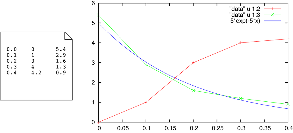
Gnuplot makes it easy to combine multiple curves on one plot. Assume that the data file looks like the one shown in Figure B-1 (left). Then the following command would plot the values of both the second and the third column, together with a function, in a single graph (Figure B-1, right):

plot "data" u 1:2 w lp, "data" u 1:3 w lp, 5*exp(-5*x)

Here we have made use of the fact that many directives can be abbreviated (u for using and w for with) and have also introduced a new plotting style, linespoints (abbreviated lp), which plots values as symbols connected by lines. The other two most important styles are lines, or l, which connects data points with straight lines but does not plot symbols, and points, or p, which plots only symbols but no lines.

Figure B-1. A data file (left) and the resulting plot (right).

It is possible to modify the ranges of values included in a plot (“zooming”) by using range specifiers as follows.

plot [0:0.5] plot "data" using 1:2 w p
plot [0:0.5][0:7] plot "data" using 1:2 w lp
plot [][0:7] plot "data" using 1:2 w l

The first line would limit the x range, the second line would limit both the x range and the y range, and the third line would limit only the y range.

Gnuplot is, by design, only a plotting utility; it is not a general-purpose computational workbench (like Matlab, Octave, R, and many others). Nevertheless, it is possible and often useful to apply a transformation to data points as they are being plotted.

The following code will plot the square root of the second column:

plot "data" using 1:(sqrt($2)) with lines

Whenever the column specification in the using directive is enclosed in parentheses, the contents of the parentheses are evaluated as a mathematical expression. When inside parentheses, you can access column values by preceding the column number with a dollar sign ($). The basic arithmetic operations are supported, as are all standard (and some not-so-standard) mathematical functions.

The simulation framework introduced in Chapter 12 writes results out (to standard output) in a format that is suitable for gnuplot. Assuming that standard output has been redirected to a file called results, the setpoint (column 3) and the actual plant output (column 7) can be plotted as a function of the wall-clock time (column 2) with a command like this:

plot "results" using 2:3 with lines, "" u 2:7 w l

Notice how the filename has been left blank the second time, in which case gnuplot reuses the most recently given filename.

These instructions should be sufficient to allow you to make basic plots. Extensive documentation is available within a gnuplot session using the help command:

help plot

The same information can also be found as a PDF on the gnuplot website.

In addition to the basic plot command, gnuplot provides myriad of options to change the appearance of a plot or to add annotations to it. A systematic introduction can be found, for instance, in my book on gnuplot.^[34]