For phenomena occurring in the physical world (mechanical, electrical, chemical processes, and so on), “time” is an absolute concept: it just passes, and things happen according to laws of nature. For computer systems, things are not as clear because computer systems do not necessarily “evolve” by themselves according to separate and fixed laws. A software process waiting for an event does not “evolve” at all while it waits for an event to occur on the expected port! (Anybody who has ever had to deal with a “hung” computer will recognize this phenomenon.) So when designing control systems for computer systems, we have a degree of freedom that most control engineers do not—namely, a choice of time.

This is a consequence of using a digital controller. Classical, analog control systems were built using physical elements (springs and dampers, pipes and valves, resistors and capacitors). These control systems were subject to the same laws of nature as the systems they controlled, and their action progressed continuously in time. Digital controllers do not act continuously; they advance only in discrete time steps (almost always using time steps of fixed length, although that is not strictly required). If the controlled system itself is also digital and therefore governed by the rules of its application software, then this introduces an additional level of freedom.

There are basically two ways that time evolution for computer systems can be designed: real time or control time.

When we are trying to control a process in the physical world, only the first approach is feasible: the system evolves according to its own laws, and we must make sure that our control actions keep up with it. But when developing a control strategy for an event-driven system, the second approach may be more natural. (In Chapter 13 we will see an example of “event” time; in Chapter 17 we will see how to connect simulation parameters with “wall-clock” time.)

In a simulation, time naturally progresses in discrete steps. Therefore, the (integer) number of simulation steps is the natural way to tell time. The problem is how to make contact with the physical world that the simulation is supposed to describe.

In the following, we will assume that each simulation step has exactly the same duration when measured in wall-clock time. (This precludes event-driven situations, where the interval between successive events is a random quantity.) Each step in the simulation corresponds to a specific duration in the real world. Hence we need a conversion factor to translate simulation steps into real-world durations.

In the simulation framework, this conversion factor is implemented as a variable DT, which is global to the feedback package. This variable gives the duration (in wall-clock time) of a single simulation step and must be set before a simulation can be run. (For instance, if you want to measure time in seconds and if each simulation step is supposed to describe 1/100 of a second, then you would set DT = 0.01. If you measure time in days and take one simulation step per day, then DT = 1.)

The factor DT enters calculations in the simulation framework in two ways. First, the convenience functions for standard loops (see later in this chapter) write out simulation results at each step for later analysis, including both the (integer) number of simulation steps and the wall-clock time since the beginning of the simulation. (The latter is simply DT multiplied by the number of simulation steps.) The second way that DT enters the simulation results is in the calculation of integrals and derivatives, both of which are approximated by finite differences:

 

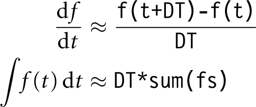
where fs = [ f0, f1, f2, ... ] is a sequence holding the values of f(t) for all simulation steps so far.

It is a separate question how long or short (in wall-clock time) you should choose the duration of each simulation step to be. In general, you want each simulation step to be shorter by at least a factor of 5 to 10 than the dominant time scale of the system that you are modeling (see Chapter 10). This is especially important when simulating systems described by differential equations, since it ensures that the finite-difference approximation to the derivatives is reasonably accurate.

All components that can occur in a simulation are subclasses of Component in package feedback. This base class provides two functions, which subclasses should override. The work() function takes a single scalar argument and returns a single scalar return value. This function encapsulates the dynamic function of the component: it is called once for each time step. Furthermore, a monitoring() function, which takes no argument, can be overridden to return an arbitrary string that represents the component’s internal state. This function is used by some convenience functions (which we’ll discuss later in this chapter) and allows a uniform approach to logging. Having uniform facilities for these purposes will prove convenient at times.

The complete implementation of the Component base class looks like this:

class Component:
    def work( self, u ):
        return u

    def monitoring( self ):
        # Overload, to print addtl monitoring info to stdout
        return ""

All implementation of “plants” or systems that we want to control in simulations should extend the Component base class and override the work() function (and the monitoring() function, if needed):

class Plant( Component ):
    def work( self, u ):
        # ... implentation goes here

We will see many examples in the chapters that follow.

The feedback package provides an implementation of the standard PID controller as a subclass of the Component abstraction. Its constructor takes values for the three controller gains (k_p, k_i, and k_d; the last one defaults to zero). The work() function increments the integral term, calculates the derivative term as the difference between the previous and the current value of the input, and finally returns the sum of the contributions from all three terms:

class PidController( Component ):
    def __init__( self, kp, ki, kd=0 ):
        self.kp, self.ki, self.kd = kp, ki, kd
        self.i = 0
        self.d = 0
        self.prev = 0

    def work( self, e ):
        self.i += DT*e
        self.d = ( e - self.prev )/DT
        self.prev = e

        return self.kp*e + self.ki*self.i + self.kd*self.d

Observe that the factor DT enters the calculations twice: in the integral term and when approximating the derivative by the finite difference between the previous and the current error value.

A more advanced implementation is provided by the class AdvController. Compared to the PidController, it has two additional features: a “clamp” to prevent integrator windup and a filter for the derivative term. By default, the derivative term is not smoothed; however, by supplying a positive value less than 1 for the smoothing parameter, the contribution from the derivative term is smoothed using a simple recursive filter (single exponential smoothing).

The clamping mechanism is intended to prevent integrator windup. If the controller output exceeds limits specified in the constructor, then the integral term is not updated in the next time step. The limits should correspond to the limits of the “actuator” following the controller. (For instance, if the controller were controlling a heating element, then the lower boundary would be zero, since it is in general impossible for a heating element to produce negative heat flow.) This clamping mechanism has been chosen for the simplicity of its implementation—many other schemes can be conceived.

class AdvController( Component ):
    def __init__( self, kp, ki, kd=0,
                  clamp=(-1e10,1e10), smooth=1 ):
        self.kp, self.ki, self.kd = kp, ki, kd
        self.i = 0
        self.d = 0
        self.prev = 0

        self.unclamped = True
        self.clamp_lo, self.clamp_hi = clamp

        self.alpha = smooth

    def work( self, e ):
        if self.unclamped:
            self.i += DT*e

        self.d = ( self.alpha*(e - self.prev)/DT +
                   (1.0-self.alpha)*self.d )

        u = self.kp*e + self.ki*self.i + self.kd*self.d

        self.unclamped = ( self.clamp_lo < u < self.clamp_hi )
        self.prev = e

        return u

Various other control elements can be conceived and implemented as subclasses of Component. The Identity element simply reproduces its input to its output—it is useful mostly as a default argument to several of the convenience functions:

class Identity( Component ):
    def work( self, x ): return x

More interesting is the Integrator. It maintains a cumulative sum of all its inputs and returns its current value:

class Integrator( Component ):
    def __init__( self ):
        self.data = 0

    def work( self, u ):
        self.data += u
        return DT*self.data

Because the Integrator class is supposed to calculate the integral of its inputs, we need to multiply the cumulative term by the wall-clock time duration DT of each simulation step.

Finally, we have two smoothing filters. The FixedFilter calculates an unweighted average over its last n inputs:

class FixedFilter( Component ):
    def __init__( self, n ):
        self.n = n
        self.data = []

    def work( self, x ):
        self.data.append(x)

        if len(self.data) > self.n:
            self.data.pop(0)

        return float(sum(self.data))/len(self.data)

The RecursiveFilter is an implementation of the simple exponential smoothing algorithm

that mixes the current raw value x_t and the previous smoothed value s_t–1 to obtain the current smoothed value s_t:

class RecursiveFilter( Component ):
    def __init__( self, alpha ):
        self.alpha = alpha
        self.y = 0

    def work( self, x ):
        self.y = self.alpha*x + (1-self.alpha)*self.y
        return self.y

Because all these elements adhere to the interface protocol defined by the Component base class, they can be strung together in order to create simulations of multi-element loops.

In addition to various standard components, the framework also includes convenience functions to describe several standard control loop arrangements in the feedback package. The functions take instances of the required components as arguments and then perform a specified number of simulation steps of the entire control system (or control loop), writing various quantities to standard output for later analysis. The purpose of these functions is to reduce the amount of repetitive “boilerplate” code in actual simulation setups.

The closed_loop() function is the most complete of these convenience functions. It models a control loop such as the one shown in Figure 12-1. It takes three mandatory arguments: a function to provide the setpoint, a controller, and a plant instance. Controller and plant must be subclasses of Component. The setpoint argument must be a reference to a function that takes a single argument and returns a numeric value, which will be used as a setpoint for the loop. The loop provides the current simulation time step as an integer argument to the setpoint function—this makes it possible to let the setpoint change over time. These three arguments are required.

Figure 12-1. The control loop modeled by the closed_loop() function.

The remaining arguments have default values. There is the maximum number of simulation time steps tm and a flag inverted to indicate whether the tracking error should be inverted (e → –e) before being passed to the controller. This is necessary in order to deal with processes for which the process output decreases as the process input increases. (This mechanism allows us to maintain the convention that controller gains are always positive, as was pointed out in Chapter 4). Finally, we can insert an arbitrary actuator between the controller and the plant, or we can introduce a filter into the return path (for instance, to smooth a noisy signal). The complete implementation of the closed control loop can then be expressed in just a few lines of code:

def closed_loop( setpoint, controller, plant, tm=5000,
                 inverted=False, actuator=Identity(),
                 returnfilter=Identity() ):
    z = 0
    for t in range( tm ):
        r = setpoint(t)
        e = r - z
        if inverted == True: e = -e
        u = controller.work(e)
        v = actuator.work(u)
        y = plant.work(v)
        z = returnfilter.work(y)

        print t, t*DT, r, e, u, v, y, z, plant.monitoring()

In any case, we must provide an implementation of the plant and of the function to be used for the setpoint. Once this has been done, a complete simulation run can be expressed completely through the following code:

class Plant( Component ):
     ...

def setpoint( t ):
    return 100

p = Plant()
c = PidController( 0.5, 0.05 )

closed_loop( setpoint, c, p )

All convenience functions use the same output format. At each time step, values for all signals in the loop are written to standard output as white-space separated text. Each line has the following format:

The remaining convenience functions describe a system for conducting step-response tests and an open-loop arrangement. There is also a function that conducts a complete test to determine the static, steady-state process characteristic.

The simulation framework itself does not include functionality to produce graphs—this task is left for specialized tools or libraries. If you want to include graphing functionality directly into your simulations, then matplotlib is one possible option.

The alternative is to dump the simulation results into a file and to use a separate graphing tool to plot them. The graphs for this book were created using gnuplot, although many other comparable tools exist. You should pick the one you are most comfortable with. (As a starting point, a brief tutorial on gnuplot is included in Appendix B.)