A.3. Stream Ciphers

A block cipher encrypts large blocks of data using a fixed key. A stream cipher, on the other hand, encrypts small blocks of data (typically bits or bytes) using different keys. The security of a stream cipher stems from the unpredictability of guessing the keys in the key stream. Here, we deal with stream ciphers that encrypt bit-by-bit.

Definition A.2.

Example A.1.

Generating a truly random key stream of arbitrary length is a difficult problem. Moreover, the same key stream is used for decryption and has to be reproduced at the recipient’s end. In view of these difficulties, Vernam’s one-time pad is used only very rarely.

A practical solution is to use a pseudorandom key stream k₁, k₂, k₃, . . . generated from a secret key J of fixed small length. The bits in the pseudorandom stream should be sufficiently unpredictable and the length of J adequately large, so as to preclude the possibility of mounting a successful attack in feasible time.

Depending on how the key stream is generated from J, stream ciphers can be broadly classified in two categories. In a synchronous stream cipher, each key in the key stream is generated independent of any plaintext or ciphertext bit, whereas in a self-synchronizing (or asynchronous) stream cipher each key in the stream is generated based only on J and a fixed number of previous ciphertext bits. Algorithms A.16 and A.17 explain the workings of these two classes of stream ciphers.

Algorithm A.16. Encryption in a synchronous stream cipher

Algorithm A.17. Encryption in an asynchronous stream cipher

A block cipher in the OFB mode works like a synchronous stream cipher, whereas a block cipher in the CFB mode like an asynchronous stream cipher.

A.3.1. Linear Feedback Shift Registers

Linear feedback shift registers (LFSRs), being suitable for hardware implementation and possessing good cryptographic properties, are widely used as basic building blocks for many stream ciphers. Figure A.2 depicts an LFSR L with d stages or delay elements D₀, D₁, . . . , D_d–1, each capable of storing one bit. The state of the LFSR is described by the d-tuple s := (s₀, s₁, . . . , s_d–1), where s_i is the bit stored in D_i. It is often convenient to treat s as the column vector (s₀ s₁ . . . s_d–1)^t.

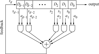
There are d control bits a₀, a₁, . . . , a_d–1. The working of the LFSR is governed by a clock. At every clock pulse the bits stored in the delay elements are bit-wise AND-ed with the respective control bits and the AND gate outputs are XOR-ed to obtain the bit s_d. The bit s₀ stored in D₀ is delivered to the output. Finally, for each the delay element D_i sets its stored bit to s_i+1, that is, the register experiences a right shift by one bit with the feedback bit s_d filling up the leftmost delay element.

Thus, a clock pulse changes the state of the LFSR from s := (s₀, s₁, . . . , s_d–1) to t := (t₀, t₁, . . . , t_d–1), where s and t are related as:

If s and t are treated as column vectors, this can be compactly represented as

Equation A.4

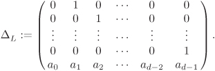
where the transition matrix Δ_L is given by

Equation A.5

When the LFSR L is initialized to a non-zero state, the bit stream output by it can be used as a pseudorandom bit sequence. For a given set of control bits a₀, . . . , a_d–1, the next state of L is uniquely determined by its previous state only. Since L has only finitely many (2^d – 1) non-zero states, the output bit sequence of L must be (eventually) periodic. For cryptographic use, the period of the bit sequence should be as large as possible. If the period is maximum possible, namely 2^d – 1, L is called a maximum-length LFSR.

Many properties of the LFSR L can be explained in terms of its connection polynomial defined as:

Equation A.6

For example, assume that a₀ = 1, so that deg C_L(X) = d. Assume further that C_L(X) is irreducible (over ). Consider the extension of , represented as , where . It turns out that if x is a generator of the cyclic group , then L is a maximum-length LFSR. In this case, the polynomial C_L(X) is called a primitive polynomial of .^[3]

^[3] A primitive polynomial defined in this way has nothing to do with a primitive polynomial over a UFD, defined in Exercise 2.54. Mathematicians often go for such multiple definitions of the same terms and phrases.

A.3.2. Stream Ciphers Based on LFSRs

The bit sequence output by an LFSR L can be used as the key stream k₁k₂ . . . k_l in order encrypt a plaintext stream m₁m₂ . . . m_l to the ciphertext stream c₁c₂ . . . c_l with c_i := m_i ⊕ k_i. The number d of stages in L should be chosen reasonably large and the control bits a₀, . . . , a_d–1 should be kept secret. The initial state of L may or may not be a secret. For suitable choices of a₀, . . . , a_d–1, the output sequences from L possess good statistical properties and hence L appears to be an efficient key stream generator.

Unfortunately, such a key stream generator is vulnerable to a known-plaintext attack as follows. Suppose that m_i and c_i are known for i = 1, 2, . . . , 2d. One can easily compute k_i = m_i⊕c_i for all these i. Let s_i := (k_i, k_i+1, . . . , k_i+d–1) denote the state of L while outputting c_i. By Congruence (A.4), s_i+1 ≡ Δ_Ls_i (mod 2) for i = 1, 2, . . . , d. Define the d × d matrices S := (s₁ s₂ . . . s_d) and T := (s₂ s₃ . . . s_d+1), where s_i are treated as column vectors as before. We then have T ≡ Δ_LS (mod 2). If S is invertible modulo 2, then Δ_L and hence the secret control bits can be easily computed. In order to avoid this known-plaintext attack, one should introduce some non-linearity in the LFSR outputs.

A non-linear combination generator combines the output bits u₁, u₂, . . . , u_r from r LFSRs by a non-linear function in order to generate the key . The Geffe generator of Figure A.3 gives a well-known example. It uses the non-linear function , that is, (mod 2).

A non-linear filter generator generates the key as k = ψ(s₀, s₁, . . . , s_d–1), where s₀, . . . , s_d–1 are the bits stored in the delay elements of a single LFSR and where ψ is a non-linear function.

Several other ad hoc schemes can destroy the linearity of an LFSR’s output. The shrinking generator, for example, uses two LFSRs L₁ and L₂. Both L₁ and L₂ are simultaneously clocked. If the output of L₁ is 1, the output of L₂ goes to the key stream, whereas if the output of L₁ is 0, the output of L₂ is discarded. The resulting key stream is an irregularly (and non-linearly) decimated subsequence of the output sequence of L₂.

The non-linear function ( or ψ) eliminates the chance of mounting the straightforward known-plaintext attack described above. However, for polynomial non-linearities certain algebraic attacks are known, for example, see Courtois and Pieprzyk [67, 66].^[4] Solving non-linear polynomial equations is usually more difficult than solving linear equations, but ample care should be taken to avoid accidental encounters with easily solvable systems. Complacency is a word ever excluded from a cryptologer’s world.

^[4] Visit the Internet site http://www.cryptosystem.net/ for more papers in related areas.

Exercise Set A.3

A.12	For each of the two classes of stream ciphers (Algorithms A.16, A.17) discuss the effects on decryption of alteration insertion or deletion of a ciphertext bit during transmission.
A.13	Suppose that the LFSR L of Figure A.4 is initialized to the state (1, 0, 0, 0). Derive the sequence of state transitions of the LFSR, and hence determine the output bit sequence of L. Argue that L is a maximum-length LFSR. Verify (according to the definition) that the connection polynomial CL(X) is primitive. Figure A.4. An LFSR with four stages
A.14	Let ΔL and CL(X) be as in Equations (A.5) and (A.6). Show that: ΔL is invertible modulo 2 if and only if a0 = 1. The characteristic polynomial of ΔL (a matrix over ) is XdCL(1/X). [H]
A.15	Let L be an LFSR with connection polynomial CL(X). Further let , , denote a power series[5] over . Show that L generates the (infinite) bit sequence s0, s1, s2, . . . if and only if the product CL(X)S(X) modulo 2 is a polynomial of degree < d. [5] A power series over a ring A is a (formal) expression of the form with each . The set of all such power series is denoted by A[[X]]. For two power series and over A, the sum f + g is defined to be the power series and the product fg is defined as the power series , where . Under these operations A[[X]] is a ring. A polynomial over A can be identified with an element of A[[X]], in which all, but finitely many, coefficients are zero.
A.16	Let σ = s0s1 . . . sd–1 ≠ 00 . . . 0 be a bit string of length d ≥ 1. The linear complexity L(σ) of σ is defined to be the length of the shortest LFSR that generates σ as the leftmost part of its output (after it is initialized to a suitable state). Prove that: L(σ) ≤ d. L(σ) = d if and only if σ = 00 . . . 01. [H]
A.17	Assume that the three LFSR outputs u1, u2, u3 in the Geffe generator are uniformly distributed. Show that Pr(k = u1) = 3/4 = Pr(k = u3). Thus, partial information about the internal details of the Geffe generator is leaked out in the key stream.