*3.6. Arithmetic on Elliptic Curves

The recent popularity of cryptographic systems based on elliptic curve groups over stems from two considerations. First, discrete logarithms in can be computed in subexponential time. This demands q to be sufficiently large, typically of length 768 bits or more. On the other hand, if the elliptic curve E over is carefully chosen, the only known algorithms for solving the discrete logarithm problem in are fully exponential in lg q. As a result, smaller values of q suffice to achieve the desired level of security. In practice, the length of q is required to be between 160 and 400 bits. This leads to smaller key sizes for elliptic curve cryptosystems. The second advantage of using elliptic curves is that for a given prime power q, there is only one group , whereas there are many elliptic curve groups (over the same field ) with orders ranging from to . If a particular group is compromised, we can switch to another curve without changing the base field .

In this section, we start with the description of efficient implementation of the arithmetic in the groups . Then we concentrate on some algorithms for counting the order . Knowledge of this order is necessary to find out cryptographically suitable elliptic curves. We consider only prime fields or fields of characteristic 2. So we assume that the curve is defined by Equation (2.8) or Equation (2.9) on p 100 (supersingular curves are not used in cryptography) instead of by the general Weierstrass Equation (2.6) on p 98.

3.6.1. Point Arithmetic

Let us first see how we can efficiently represent points on an elliptic curve E over . Since corresponds to two elements h, and since each element of can be represented using ≤ s = ⌈lg q⌉ bits, 2s bits suffice to represent P. We can do better than this. Substituting X = h in the equation for E leaves us with a quadratic equation in Y. This equation has two roots of which k is one. If we adopt a convention (for example, see Section 6.2.1) that identifies, using a single bit, which of the two roots the coordinate k is, the storage requirement for P drops to s + 1 bits. During an on-line computation this compressed representation incurs some overhead and may be avoided. However, for off-line storage and transmission (of public keys, for example), this compression may be helpful.

Explicit formulas for the sum of two points and for the opposite of a point on an elliptic curve E are given in Section 2.11.2. These operations in can be implemented using a few operations in the ground field .

Computation of mP for and (or, more generally, for ) can be performed using a repeated-double-and-add algorithm similar to the repeated-square-and-multiply Algorithm 3.9. We leave out the trivial modifications and urge the reader to carry out the details.

Finding a random point is another useful problem. If q = p is an odd prime and we use the short Weierstrass Equation (2.8), we first choose a random and substitute X by h to get Y² = h³ + ah + b. This equation has 2, 0 or 1 solution(s) depending on whether h³ + ah + b is a quadratic residue or non-residue or 0 modulo p. Quadratic residuosity can be checked by computing the Legendre symbol (Algorithm 3.15), whereas square roots modulo p can be computed using Tonelli and Shanks’ Algorithm 3.16.

For a non-supersingular curve E over defined by Equation (2.9), a random point is chosen by first choosing a random . Substituting X = h in the defining equation gives Y² + hY + (h³ + ah² + b) = 0. If h = 0, then the unique solution for k is b^2n–1. If h ≠ 0, replacing Y by hY and dividing by h² transforms the equation to the form Y² + Y + α = 0 for some . This equation has two or zero solutions depending on whether the absolute trace is 0 or 1. If k is a solution, the other solution is k + 1. In order to find a solution (if it exists), one may use the (probabilistic) root-finding algorithm of Exercise 3.36. Another possibility is discussed now.

We consider two separate cases. First, if n is odd, then is a solution, since Tr(α) = k² + k + α. On the other hand, if n is even, we first find a with Tr(β) = 1. Since Tr is a homomorphism of the additive groups and Tr(1) = 1, exactly half of the elements of have trace 1. Therefore, a desired β can be quickly found out by selecting elements of at random and computing traces of these elements. Now, it is easy to check that gives a solution of Y² + Y + α = 0.

**3.6.2. Counting Points on Elliptic Curves

Counting points on elliptic curves is a challenging problem, both theoretically and computationally. The first polynomial time (in log q) algorithm invented by Schoof and later made efficient by Elkies and Atkins (and many others), is popularly called the SEA algorithm. Unfortunately, even the most efficient implementation of this algorithm is not quite efficient, but it is the only known reasonable strategy, in particular, when q = p is a large (odd) prime of a size of cryptographic interest. The more recent Satoh–FGH algorithm, named after its discoverer Satoh and after Fouquet, Gaudry and Harley who proposed its generalized and efficient versions, is a remarkable breakthrough for the case q = 2ⁿ. Both the SEA and the Satoh–FGH algorithms are mathematically quite sophisticated. We now present a brief overview of these algorithms.

The SEA algorithm

We assume that q = p is a large odd prime, this being the typical situation when we apply the SEA algorithm. We also assume that E is given by the short Weierstrass equation Y² = X³ + aX + b. Let q₁ = 2, q₂ = 3, q₃ = 5, . . . be the sequence of prime numbers and t the Frobenius trace of E at p. By Hasse’s theorem (Theorem 2.48, p 106), with . A knowledge of t modulo sufficiently many small primes l allows us to reconstruct t using the Chinese remainder theorem. Because of the Hasse bound on t, it is sufficient to choose l from the primes q₁, q₂, . . . in succession, until the product q₁q₂ · · · q_r exceeds . By the prime number theorem (Theorem 2.20, p 53), we have r = O(ln p) and also q_i = O(ln p) for each i = 1, . . . , r.

The most innovative idea of Algorithm 3.31 is the determination of the integers t_i. For l = q₁ = 2, the process is easy. We have t₁ ≡ t ≡ 0 (mod 2) if and only if contains a point of order 2 (a point of the form (h, 0)), or equivalently, if and only if the polynomial X³ + aX + b has a root in . We compute the polynomial gcd g(X) := gcd(X³ + aX + b, X^p–X) over and conclude that

Algorithm 3.31. SEA algorithm for elliptic curve point counting

Determination of t_i for i > 1 involves more work. We explain here the original idea due to Schoof. We denote by l the i-th prime q_i and by the set of all l-torsion points of (Definition 2.78, p 105). The Frobenius endomorphism that maps and to (h^p, k^p) satisfies the relation . If we restrict our attention only to the group E[l], then this relation reduces to , where t_i = t rem l and p_i = p rem l, that is, for all .

In terms of polynomials, the last relation is equivalent to

Equation 3.4

where the sum and difference follow the formulas for the elliptic curve E. Now, one has to calculate symbolically rather than numerically, since X and Y are indeterminates. These computations can be carried out in the ring (instead of in ), where f(X, Y) = Y² – (X³ + aX + b) is the defining polynomial of E and f_l = f_l(X) is the l-th division polynomial of E (Section 2.11.2 and Theorem 2.47, p 106). Reduction of a polynomial in modulo f makes its Y-degree ≤ 1, whereas reduction modulo f_l makes the X-degree less than deg f_l which is O(l²). We can try the values t_i = 0, 1, . . . , l – 1 successively until the desired value satisfying Equation (3.4) is found out.

It is not difficult to verify that Schoof’s algorithm runs in time O(log⁸ p) (under standard arithmetic in ) and is thus a deterministic polynomial-time algorithm for the point-counting problem. Essentially the same algorithm works for fields with q = 2ⁿ and has the same running time. Unfortunately, the big exponent (8) in the running time makes Schoof’s algorithm quite impractical. Numerous improvements are suggested to bring down this exponent. Elkies and Atkin’s modification for the case q = p gives rise to the SEA algorithm which has a running time of O(log⁶ p) under the standard arithmetic in . This speed-up is achieved by working in the ring , where g_l is a suitable factor of f_l and has degree O(l). Couveignes suggests improvements for the fields of characteristic 2. Efficient implementations of the SEA algorithm are reported by Morain, Müller, Dewaghe, Vercauteren and many others. At the time of writing this book, the largest values of q for which the algorithm has been successfully applied are 10⁴⁹⁹ + 153 (a prime) and 2¹⁹⁹⁹ (a power of 2).

The Satoh–FGH algorithm

The Satoh–FGH algorithm is well suited for fields of small characteristic p and, in particular, for the fields of characteristic 2. This algorithm has enabled point-counting over fields as large as . A generic description of the Satoh–FGH algorithm now follows after the introduction of some mathematical notions. Though our practical interest concentrates on the fields only, we consider curves over a general with q = pⁿ, p a prime.

Recall from Section 2.14 that the ring of p-adic integers is a discrete valuation ring (Exercises 2.133 and 2.148) with the unique maximal ideal generated by , and the residue field is isomorphic to .

We represent as a polynomial algebra over . We analogously define the p-adic ring , where f is an irreducible polynomial of degree n in . The elements of can be viewed as polynomials of degrees < n and with p-adic integers as coefficients. The arithmetic operations in are polynomial operations in modulo the defining polynomial f. The ring is canonically embedded in the ring (consider constant polynomials).

turns out to be a discrete valuation ring with maximal ideal , and the residue field is isomorphic to .

Definition 3.6.

The p-th power Frobenius endomorphism , a ↦ a^p, can now be extended to an endomorphism as follows. Let have the semi-Witt decomposition a₀, a₁, . . . with . Then, is the unique element having the semi-Witt decomposition One can show that . We have and similarly .

Now, let E = E₀ be an elliptic curve defined over . Application of to the coefficients of E₀ gives another elliptic curve E₁ over whose rational points are , , where , together with the point at infinity. We may apply to E₁ to get another curve E₂ over and so on. Since , we get a cycle of elliptic curves defined over :

Equation 3.5

Similarly, if ε = ε₀ is an elliptic curve defined over , application of leads to a sequence of elliptic curves defined over :

Equation 3.6

We need the canonical lifting of an elliptic curve E over to a curve ε over . Explaining that requires some more mathematical concepts:

Definition 3.7.

Theorem 3.4.

Definition 3.8.

The next theorem establishes the foundation for lifting curves from to .

Theorem 3.5. Lubin–Serre–Tate

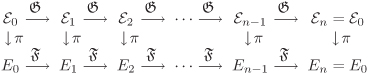
With this definition of lifting of elliptic curves, Cycles (3.5) and (3.6) satisfy the following commutative diagram, where ε_i is the canonical lift of E_i for each i = 0, 1, . . . , n.

Algorithm 3.32 outlines the Satoh–FGH algorithm. In order to complete the description of the algorithm, one should specify how to lift curves (that is, a procedural equivalent of Theorem 3.5) and their p-torsion points and how the lifted data can be used to compute the Frobenius trace t. We leave out the details here.

Algorithm 3.32. Satoh–FGH algorithm for elliptic curve point counting

The elements of (and hence of ) are infinite sequences and hence cannot be represented in computer memory. However, we make an approximate representation by considering only the first m terms of the sequences representing elements of . Working in with this approximate representation is then essentially the same as working in . For the Satoh–FGH algorithm, we need m ≈ n/2.

For small p (for example, p = 2) and with standard arithmetic in , the Satoh–FGH algorithm has a deterministic running time O(n⁵) and space requirement O(n³). With Karatsuba arithmetic the exponent in the running time drops from 5 to nearly 4.17. In addition, this algorithm is significantly easier to implement than optimized versions of the SEA algorithm. These facts are responsible for a superior performance of the Satoh–FGH algorithm over the SEA algorithm (for small p).

3.6.3. Choosing Good Elliptic Curves

Choosing cryptographically suitable elliptic curves is more difficult than choosing good finite fields. First, the order of the elliptic curve group must have a suitably large prime divisor, say, of bit length 160 or more. In addition, the MOV attack applies to supersingular curves and the anomalous attack to anomalous curves (Definition 2.80 and Section 4.5). So a secure curve must be non-supersingular and non-anomalous. Checking all these criteria for a random curve E over requires the group order . One may use either the SEA algorithm or the Satoh–FGH algorithm to compute . Once is known, it is easy to check whether E is supersingular or anomalous. But factoring to find its largest prime divisor may be a difficult task and is not recommended. One may instead extract all the small prime factors of by trial divisions with the primes q₁ = 2, q₂ = 3, q₃ = 5, . . . , q_r for a predetermined r and write where m₁ has all prime factors ≤ q_r and m₂ has all prime factors > q_r. If m₂ is prime and of the desired size, then E is treated as a good curve. Algorithm 3.33 illustrates these steps.

The computation of the group orders takes up most of the execution time of the above algorithm. It is, therefore, of utmost importance to employ good algorithms for point counting. The best algorithms known till date (the SEA and the Satoh–FGH algorithms) are only reasonable. Further research in this area may lead to better algorithms in future.

Algorithm 3.33. Selecting cryptographically suitable elliptic curves

There are ways of generating good curves without requiring the point counting algorithms over large finite fields. One possibility is to use the so-called subfield curves. If has a subfield of relatively small cardinality, one can choose a random curve E over and compute . Since E is also a curve defined over and can be easily obtained using Theorem 2.51 (p 107), we save the lengthy direct computation of . However, the drawback of this method is that since E is now chosen with coefficients from a small field , we do not have many choices. The second drawback is that we must have a small divisor q′ of q. If q is already a prime, this strategy does not work at all. If q = pⁿ, p a small prime, we need n to have a small divisor n′ that corresponds to q′ = p^n′. Sometimes small odd primes p are suggested, but the arithmetic in a non-prime field of some odd characteristic is inherently much slower than that in a field of nearly equal size but of characteristic 2.

Specific curves with complex multiplication (Definition 3.7) over large prime fields have also been suggested in the literature. Finding good curves with complex multiplication involves less computational overhead than Algorithm 3.33, but (like subfield curves) offers limited choice. However, it is important to mention that no special attacks are currently known for subfield curves and also for those chosen by the complex multiplication strategy.