
B.6. Polynomial-pool-based Key Predistribution
Liu and Ning’s polynomial-pool-based key predistribution scheme (abbreviated as the poly-pool scheme) [181, 183] is based on the idea presented by Blundo et al. [28]. Let ![]() be a finite field with q just large enough to accommodate a symmetric encryption key. For a 128-bit block cipher, one may take q to be smallest prime larger than 2128 (prime field) or 2128 itself (extension field of characteristic 2). Let
be a finite field with q just large enough to accommodate a symmetric encryption key. For a 128-bit block cipher, one may take q to be smallest prime larger than 2128 (prime field) or 2128 itself (extension field of characteristic 2). Let ![]() be a bivariate polynomial that is assumed to be symmetric, that is, f(X, Y) = f(Y, X). Let t be the degree of f in each of X and Y. A polynomial share of f is a univariate polynomial f(α)(X) := f(X, α) for some element
be a bivariate polynomial that is assumed to be symmetric, that is, f(X, Y) = f(Y, X). Let t be the degree of f in each of X and Y. A polynomial share of f is a univariate polynomial f(α)(X) := f(X, α) for some element ![]() . Two shares f(α) and f(β) of the same polynomial f satisfy
. Two shares f(α) and f(β) of the same polynomial f satisfy
Equation B.6
![]()
Thus, if the shares f(α), f(β) are given to two nodes, they can come up with the common value ![]() as a shared secret between them.
as a shared secret between them.
Given t + 1 or more shares of f, one can reconstruct f(X, Y) uniquely using Lagrange’s interpolation formula (Exercise 2.53). On the other hand, if only t or less shares are available, there are many (at least q) possibilities for f and it is impossible to determine f uniquely. So the disclosure of up to t shares does not reveal the polynomial f to an adversary and uncompromised shared keys based on f remain secure.
Using a single polynomial for the entire network is not a good proposal, since t is limited by memory constraints in a sensor node. In order to increase resilience against node captures, many bivariate polynomials need to be used, and shares of random subsets of this polynomial pool are assigned to the key rings of individual nodes. This is how the poly-pool scheme works. If the degree t equals 0, this scheme degenerates to the EG scheme.
The key set-up server first selects a random pool ![]() of S symmetric bivariate polynomials in
of S symmetric bivariate polynomials in ![]() each of degree t in X and Y. Some IDs
each of degree t in X and Y. Some IDs ![]() are also generated for the nodes in the network. For each node u in the network, s polynomials f1, f2, . . . , fs are randomly picked up from
are also generated for the nodes in the network. For each node u in the network, s polynomials f1, f2, . . . , fs are randomly picked up from ![]() and the polynomial shares f1(X, α), f2(X, α), . . . , fs(X, α) are loaded in the key ring of u, where α is the ID of u. Each key ring now requires space for storing s(t + 1) log q bits, that is, for storing m := s(t + 1) symmetric keys.
and the polynomial shares f1(X, α), f2(X, α), . . . , fs(X, α) are loaded in the key ring of u, where α is the ID of u. Each key ring now requires space for storing s(t + 1) log q bits, that is, for storing m := s(t + 1) symmetric keys.
Upon deployment, each node u broadcasts the IDs of the polynomials, the shares of which reside in its key ring. Each physical neighbour v of u, that has shares of some common polynomial(s), establishes itself as a direct neighbour of u. The exact pairwise key k between u and v is then calculated using Equation (B.6). If broadcasting polynomial IDs in plaintext is too unsafe, each node u can send some message encrypted by potential pairwise keys based on its polynomial shares. Those physical neighbours that can decrypt one of these encrypted messages have shares of common polynomials.
Like the EG scheme, the poly-pool scheme can be analysed under the framework of random graphs. Equations (B.1), (B.2) and (B.3) continue to hold under the poly-pool scheme. However, in this case the local connection probability p′ is computed as
Equation B.7
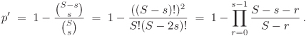
Given constraints on the network and the nodes, the desired size S of the polynomial pool ![]() can be determined from this formula.
can be determined from this formula.
Let us now compute the probability Pe of compromise of communication between two uncaptured nodes u, v as a function of the number c of captured nodes. If c ≤ t, the eavesdropper cannot gather enough polynomial shares to learn about any polynomial in ![]() , that is, Pe = 0. So assume that c > t and let pr denote the probability that exactly r shares of a given polynomial f (say, the one whose shares are used by the two uncaptured nodes u, v) are available in the key rings of the c captured nodes. The probability that a share of f is present in a key ring is
, that is, Pe = 0. So assume that c > t and let pr denote the probability that exactly r shares of a given polynomial f (say, the one whose shares are used by the two uncaptured nodes u, v) are available in the key rings of the c captured nodes. The probability that a share of f is present in a key ring is ![]() and so (by the Bernoulli distribution)
and so (by the Bernoulli distribution)
Equation B.8
![]()
Since t + 1 or more shares of f are required for the determination of f, we have
Equation B.9
![]()
Example B.6.
|
Let n = 10,000 (network size), n′ = 50 (expected size of physical neighbourhood of a node), m = 150 (key ring size in number of symmetric keys) and Pc = 0.9999 (global connectivity). Let us plan to choose bivariate polynomials of degree t = 49, so that each key ring can hold s = 3 polynomial shares. For the determination of S, we first compute d = 20 as in Example B.1. We then require The following table lists the probability Pe for various values of c.
The table shows substantial improvement in resilience against node capture as achieved by the poly-pool scheme over the EG and qC schemes. |
B.6.1. Pairwise Key Predistribution
The poly-pool scheme can be made pairwise by allowing no more than t + 1 shares of any polynomial to be distributed among the nodes. The best that the adversary can achieve is a capture of nodes with all these t + 1 shares and a subsequent determination of the corresponding bivariate polynomial. But this knowledge does not help the adversary, since no other node in the network uses a share of this compromised polynomial. That is, two uncaptured nodes continue to communicate with perfect secrecy.
However, like the random pairwise scheme, the pairwise poly-pool scheme suffers from the drawback that the maximum supportable network size is now limited by the quantity ![]() . For the parameters of Example B.6, this size turns out to be an impractically low 333.
. For the parameters of Example B.6, this size turns out to be an impractically low 333.
B.6.2. Grid-based Key Predistribution
The grid-based key predistribution considerably enhances the resilience of the network against node captures. To start with, let us play a bit with Example B.6.
Example B.7.
|
Take n = 10,000, n′ = 50 and m = 150. We calculated that the optimal value of S that keeps the network connected with high probability is S = 20. Now, let us instead take a much bigger value of S, say, S = 200. First, let us look at the brighter side of this choice. The probability Pe is listed in the following table as a function of c.
That is a dramatic improvement in the resilience figures. It, however, comes at a cost. The optimal value S = 20 was selected in Example B.6 in order to achieve a desired connectivity in the network. With S = 200, the probability p′ reduces from 0.404 to |
The grid-based key predistribution allocates polynomial shares cleverly to the nodes so as to achieve resilience figures of the last example with a reasonable guarantee that the resulting network remains connected. Let n be the size of the network and take ![]() . For the sake of simplicity, let us assume that n = σ2. The n nodes are then placed on a σ × σ square grid. The node at the (i, j)-th grid location (where i,
. For the sake of simplicity, let us assume that n = σ2. The n nodes are then placed on a σ × σ square grid. The node at the (i, j)-th grid location (where i, ![]() ) is identified by the pair (i, j). The set-up server generates 2σ random symmetric bivariate polynomials
) is identified by the pair (i, j). The set-up server generates 2σ random symmetric bivariate polynomials ![]() , each of degree t in both X and Y. The i-th polynomial
, each of degree t in both X and Y. The i-th polynomial ![]() corresponds to the i-th row and the j-th polynomial
corresponds to the i-th row and the j-th polynomial ![]() to the j-th column in the grid. The key ring of the node at location (i, j) in the grid is given the two polynomial shares
to the j-th column in the grid. The key ring of the node at location (i, j) in the grid is given the two polynomial shares ![]() and
and ![]() . The memory required for this is equivalent to the storage for 2(t + 1) symmetric keys.
. The memory required for this is equivalent to the storage for 2(t + 1) symmetric keys.
Now, look at the key establishment phase. Let two nodes u, v with IDs (i, j) and (i′, j′) be physical neighbours after deployment. First, consider the simple case i = i′. Both the nodes have shares of the polynomial ![]() and can arrive at the common secret value
and can arrive at the common secret value ![]() using the column identities of one another. Similarly, if j = j′, the nodes can compute the shared secret
using the column identities of one another. Similarly, if j = j′, the nodes can compute the shared secret ![]() . It follows that each node can establish keys directly with 2(σ – 1) other nodes in the network. That’s, however, a truly small fraction of the entire network.
. It follows that each node can establish keys directly with 2(σ – 1) other nodes in the network. That’s, however, a truly small fraction of the entire network.
Assume now that i ≠ i′ and j ≠ j′. If the node w with identity either (i, j′) or (i′, j) is in the physical neighbourhood of both u and v, then there is a secure link between u and w, and also one between w and v. The nodes u and v can then establish a path key via the intermediate node w.
So suppose also that neither (i, j′) nor (i′, j) resides in the communication ranges of both u and v. Consider the nodes w1 := (i, k) and w2 := (i′, k) for some ![]() . Suppose further that w1 is in the physical neighbourhood of u, w2 in that of w1 and v in that of w2. But then there is a secure u, v-path comprising the links u → w1, w1 → w2 and w2 → v. Similarly, the nodes (k, j) and (k, j′) for each k ≠ i, i′ can help u and v establish a path key. To sum up, there are 2(σ – 2) potential three-hop paths between u and v.
. Suppose further that w1 is in the physical neighbourhood of u, w2 in that of w1 and v in that of w2. But then there is a secure u, v-path comprising the links u → w1, w1 → w2 and w2 → v. Similarly, the nodes (k, j) and (k, j′) for each k ≠ i, i′ can help u and v establish a path key. To sum up, there are 2(σ – 2) potential three-hop paths between u and v.
If all these three-hop paths fail, one may go for four-hop, five-hop, . . . paths, but at the cost of increased communication overhead. As argued in Liu and Ning [181, 183], exploring paths with ≤ 3 hops is expected to give the network high connectivity.
For the grid-based scheme, we have S = 2σ (the key pool size) and s = 2 (the number of polynomial shares in each node’s key ring). Thus, the probability Pe can now be derived like Equations (B.8) and (B.9) as
Pe = 1 – (p0 + p1 + · · · + pt) = pt+1 + pt+2 + · · · + pc,
where
![]()
Example B.8.
|
Take n = 10,000 and m = 150. Since each node has to store only two polynomial shares, we now take t = 74. Moreover, σ = 100, that is, the size of the polynomial pool is S = 200. The probability Pe can now be tabulated as a function of c (number of nodes captured) as follows:
This is a very pretty performance. The capture of even 60 per cent of the nodes leads to a compromise of only 3.34 per cent of the communication among uncaptured nodes. |
This robustness of the grid-based distribution comes at a cost, though. The path key establishment stage is communication-intensive and is mandatory for ensuring good connectivity. Moreover, this stage is based on the assumption that during bootstrapping not many nodes are captured. If this assumption cannot necessarily be enforced, the scheme forfeits much of its expected resilience guarantees.