8.2. Quantum Computation

We start with a formal description of quantum computation. Quantum mechanical laws govern this paradigm. We will pay little attention to the physical interpretations of these laws. A mathematical formulation suffices for our purpose.

For defining a quantum mechanical system, we need to enrich our mathematical vocabulary. Let V be a vector space over (or ). Using Dirac’s ket notation we denote a vector ψ in V as |ψ〉.

Definition 8.1.

An inner product (also called a dot product or a scalar product) on V is a function satisfying the following properties: Positivity For any , the inner product 〈ψ|ψ〉 is real and non-negative. Moreover, 〈ψ|ψ〉 = 0 if and only if |ψ〉 = 0. Linearity For a1, and |ψ〉, , we have . Skew symmetry For any |ψ〉, , we have , where the bar denotes complex conjugate. A vector space V with an inner product is called an inner product space.

Example 8.1.

For , the space is an inner product space with the inner product of |ψ〉 = (ψ1, . . . , ψn) and defined as

Definition 8.2.

The inner product on a vector space V induces a norm (Definition 2.115) on V: An inner product space which is complete (Definition 2.119) under the norm induced by its inner product is called a Hilbert space. We will typically consider finite-dimensional Hilbert spaces (over ) and for denote the n-dimensional Hilbert space by .

Definition 8.3.

We define an equivalence relation ~ on a Hilbert space as if and only if for some . An equivalence class under this relation is called a ray in . One typically considers a vector |ψ〉 with 〈ψ|ψ〉 = 1 as a representative of its equivalence class. Such a representative is unique up to multiplication by complex numbers of the form eiθ.

Definition 8.4.

An orthonormal basis of a Hilbert space is a subset B of with the following properties: B is a -basis of . 〈ψ|ψ〉 = 1 for every . for every pair of distinct vectors ψ, . It is customary to denote the n vectors in an orthonormal basis of by the symbols |0〉, |1〉, . . . , |n – 1〉.

Example 8.2.

|0〉 := (1, 0, 0 . . . , 0), |1〉 := (0, 1, 0, . . . , 0), . . . , |n – 1〉 := (0, 0, . . . , 0, 1) form an orthonormal basis of under the inner product of Example (8.1).

8.2.1. System

The following axiom describes the model of a quantum mechanical system.

Axiom 8.1. First axiom of quantum mechanics

A system is a ray in a (finite-dimensional) Hilbert space (over ).

Definition 8.5.

The simplest non-trivial quantum mechanical system is a ray in a 2-dimensional Hilbert space . Such a system is assumed to be the basic building block of a quantum computer and is called a quantum bit or a qubit. In order distinguish a qubit from a classical bit, we call the latter a cbit.

has an orthonormal basis {|0〉, |1〉}. In the classical interpretation, a cbit can assume only the two values |0〉 and |1〉, whereas a qubit can assume any value of the form

a|0〉 + b|1〉

with

a, , |a|2 + |b|2 = 1.

Such a state of the qubit is called a superposition of the classical states.

Though we don’t care much, at least for the moment, here are two promising candidates for realizing a qubit:

• Spin of an electron: The spin of a particle (like electron) in a given direction, say, along the Z-axis, is modelled as a quantum mechanical system with an orthonormal basis consisting of spin up and spin down.

• Polarization of a photon: Photons constitute another class of quantum systems, where the two independent states are provided by the polarization of a photon.

A conceptual example of a 2-state quantum system is the Schrödinger cat. The two independent states of a cat, as we classically know, are |alivei〉 and |deadi〉. However, if we think of the cat confined in a closed room and isolated from our observations, quantum mechanics models the state of the cat as a superposition (that is, a complex-linear combination) of these two states. But then if the quantum model were true, opening the room may reveal the cat in a non-trivial state a|alive〉 + b|dead〉 for some complex numbers a, b with |a|² + |b|² = 1. It would indeed be an exciting experience. But alas, quantum mechanics precludes the possibility of such an observation. Read on to know what we would actually see, if we open the room.

8.2.2. Entanglement

A single qubit is too small to build a useful computer. We need to use several (albeit a finite number of) qubits and hence must have a way to describe the combined system in terms of the individual qubits. As the simplest and basis case, we first concentrate on combining two quantum systems into one.

Axiom 8.2. Second axiom of quantum mechanics

Let A and B be two quantum mechanical systems with respective Hilbert spaces and . Let {|i〉A | i = 0, . . . , m – 1} and {|j〉B | j = 0, . . . , n – 1} be orthonormal bases of these Hilbert spaces. The quantum mechanical system AB having A and B as its two parts is described by the tensor product where is an mn-dimensional Hilbert space with an orthonormal basis {|i〉A ⊗ |j〉B | i = 0, . . . ,m – 1 and j = 0, . . . , n – 1}.

It is customary to abbreviate the normalized vector |i〉_A ⊗ |j〉_B as |i〉_A|j〉_B or even as |ij〉_AB. A general state of AB is of the form

We can generalize this construction to describe a system having components A₁, . . . , A_k. If is the Hilbert space of A_i with an orthonormal basis {|j〉_i | 0 ≤ j < n_i}, the composite system A₁ · · · A_k has the n₁ · · · n_k-dimensional Hilbert space with an orthonormal basis comprising the vectors

|j₁〉₁ ⊗ |j₂〉₂ ⊗ · · · ⊗ |j_k〉_k = |j₁〉₁|j₂〉₂ · · · |j_k〉_k = |j₁j₂ . . . j_k〉

with 0 ≤ j_i < n_i for all i = 1, . . . , k.

Definition 8.6.

An n-bit quantum register is a system having exactly n qubits.

Let A₁, . . . , A_n denote the individual bits in an n-bit quantum register A. Each A_i has the Hilbert space with orthonormal basis {|0〉, |1〉}. So A has the 2ⁿ-dimensional Hilbert space with an orthonormal basis consisting of the vectors

|j₁〉 ⊗ |j₂〉 ⊗ · · · ⊗ |j_n〉 = |j₁〉|j₂〉 · · · |j_n〉 = |j₁j₂ · · · j_n〉

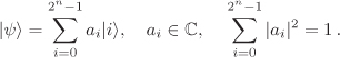
with each . Viewed as an integer in binary notation, j₁j₂ . . . j_n is an integral value between 0 and 2ⁿ – 1. This gives us a canonical numbering |0〉, |1〉, . . . , |2ⁿ – 1〉 of the basis vectors for the register A. These 2ⁿ values are precisely the states that a classical n-bit register can have. The quantum register can, however, be in any state |ψ〉 which is a superposition of the classical states:

Let us once again look at the general composite system A = A₁ · · · A_k. In the classical sense, each state of A is composed of the individual states of the subsystems A_i. For example, each of the 2ⁿ classical states of an n-bit register corresponds to a choice between |0〉 and |1〉 for each individual bit. That is, each individual component retains its own state in a classical composite system. This is, however, not the case with a quantum composite system. Just think of a 2-bit quantum register C := AB. A state

|ψ〉_C = c₀|0〉_C + c₁|1〉_C + c₂|2〉_C + c₃|3〉_C

of C equals a tensor product

|ψ1〉A ⊗ |ψ2〉B	=	(a0|0〉A + a1|1〉A) ⊗ (b0|0〉B + b1|1〉B)
	=	a0b0|0〉C + a0b1|1〉C + a1b0|2〉C + a1b1|3〉C,

if and only if c₀c₃ = c₁c₂.

Definition 8.7.

The state |ψ〉 of a quantum register A = A1 · · · An is called entangled, if |ψ〉 cannot be written as a tensor product of the states of any two parts of A. In other others, |ψ〉 is entangled if and only if no set of fewer than n qubits of A possesses its individual state.

Entanglement essentially implies correlation or interaction between the components. In a composite quantum system, we cannot treat the components individually. A quantum system, as we have defined (axiomatically) earlier, is a completely isolated system. In reality, interactions with the surroundings make a (non-isolated) system change its state and get entangled. This is one of the biggest problems in the realization of a quantum computer. Quantum error correction is an important topic in quantum computation. For our purpose, we stick to the abstract model of an isolated system (quantum register) immune from external disturbances.

8.2.3. Evolution

Quantum registers give us a way to store quantum information. A computation involves manipulating the information stored in the registers. In quantum mechanics, all such operations must be reversible, that is, it must be possible to invert every operation. The only invertible operations on the classical states |0〉, |1〉, . . . , |2ⁿ – 1〉 of an n-bit quantum register A are precisely all the permutations of the classical states. Now that A can be in many more (quantum) states, there are other allowed operations on A. Any such operation must be reversible and of a particular type. This is the third axiom of quantum mechanics, which is detailed shortly.

A classical n-bit register supports many non-invertible operations. For example, erasing the content of the register (that is, resetting all the bits to zero) is a non-invertible process, since the pre-erasure state of the register cannot be uniquely determined after the erase operation is carried out. Classical computation is based on (classical) gates (like NOT, AND, OR, XOR, NOR, NAND), most of which are non-invertible. XOR, as an example, requires two input bits and outputs a single bit. It is impossible to determine the inputs uniquely from the output only. All such non-reversible operations are disallowed in the quantum world. An invertible version of the XOR operation takes two bits x and y as input and outputs the two bits x and x ⊕ y (where ⊕ denotes XOR of bits). Given the output (x, x ⊕ y), the input can be uniquely determined as (x, y) = (x, x ⊕ (x ⊕ y)), that is, by applying the reversible XOR operation once more.

Like XOR, all bit operations that build up a classical computer can be realized using reversible operations only. This gives us the (informal) assurance that quantum computers are at least as powerful as classical computers.

Back to the business—the third axiom of quantum mechanics.

Definition 8.8.

Let U be a square matrix (that is, an m × m matrix for some ) with complex entries. The conjugate transpose of U is denoted by the symbol U†, that is, if U = (uij), then . U is called unitary, if UU† = U†U = I, where I is the m × m identity matrix. Every unitary matrix U is invertible with U–1 = U†, and preserves the inner product of , that is, for |ψ〉, .

Let A be a quantum system (like a quantum register) with Hilbert space . An m × m unitary matrix U defines a unitary linear transformation on taking a normalized vector |ψ〉 to a normalized vector U|ψ〉. Moreover, the transformation maps an orthonormal basis of to another orthonormal basis of (Exercise 8.4).

Axiom 8.3. Third axiom of quantum mechanics

A quantum system evolves unitarily, that is, any operation on a quantum mechanical system is a unitary transformation.

Example 8.3.

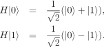
The Hadamard transform H on one qubit is defined as: (Recall that a linear transformation is completely specified by its images of the elements of a basis.) If one takes and , the Hadamard transform corresponds to the unitary matrix By linearity, H transforms a general state |ψ〉 = a|0〉 + b|1〉 to the state Some other unitary operators are described in Exercises 8.5 and 8.6.

An important consequence of quantum mechanical dynamics is that cloning of a state of a system is not permissible. In other words, there does not exist an operator that copies an arbitrary state (content) of one quantum register to another.

Theorem 8.1. No-cloning theorem

For two n-bit registers A and B, there do not exist a unitary transform U of the composite system AB and a state of B, such that for every state of |ψ〉 of A. Proof Assume that such a state of B and a unitary transform U of AB exist. Take two states |ψ1〉 and |ψ2〉 of A. Then, and . By linearity, we have . Now, since U clones |aψ1 + bψ2〉 also, . The two expressions for are different, unless a = 0, b = 1 or a = 1, b = 0.

8.2.4. Measurement

We have seen how to represent a quantum mechanical system and do operations on the system. Now comes the final part of the game, namely observing or measuring or reading the state of a quantum system. In classical computation, reading the value stored in a classical register is a trivial exercise—just read it! In quantum mechanics, this is not the case.

Axiom 8.4. Fourth axiom of quantum mechanics—the Born rule

Let A be a quantum mechanical system with an orthonormal basis {|0〉, |1〉, . . . , |m – 1〉}. Assume that A is in a state . A measurement of A at this state is a mechanism (or device) that outputs one of the integers , and i is output with probability |ai|2. If i is output by the measurement, the system collapses from the state |ψ〉 to the state |i〉 after the measurement.

This means that whatever the state |ψ〉 of A was before the measurement, the process of measurement can reveal only one of m possible integer values. Moreover, the measurement causes a total loss of information about the pre-measurement amplitudes a_i. Thus, it is impossible to measure A repeatedly at the state |ψ〉 to see a statistical pattern in the occurrences of different values of i so as to guess the probabilities |a_i|².

If we open the room, we can see the Schrödinger cat in only one of the two possible states: |alivei or |deadi. Well, then, what else can we expect? Quantum mechanics only models the cat in the isolated room as one evolving following the unitary dynamics.

At first glance, this is rather frustrating. We claim that the system went through a series of classically meaningless states, but the classical states are all we can see. What is the guarantee that the system really evolved in the quantum mechanical way? Well, there is no guarantee actually. The solace is that the axioms of quantum mechanics can explain certain natural phenomena. Also it is perfectly consistent with the classical behaviour in that if the system A evolves classically and is measured at the state |i〉 (so that a_i = 1 and a_j = 0 for j ≠ i), measuring A reveals i with probability one and causes the system to collapse to the state |i〉, that is, to remain in the state |i〉 itself.

There is a positive side of the quantum mechanical axioms. A quantum mechanical system is inherently parallel. An n-bit classical register at any point of time can hold only one of the classical values |0〉, . . . , |2ⁿ – 1〉. An n-bit quantum register, on the other hand, can simultaneously hold all these classical values, with respective probabilities. This inherent parallelism seems to impart a good deal of power to a computing device. Of course, as long as we cannot harness some physical objects to build a real quantum mechanical computing device, quantum computation continues to remain science fiction. But on an algorithmic level, the inherent parallelism of a (hypothetical) quantum computer can be exploited to do miracles, for example, to design a polynomial-time integer factorization algorithm. This is where we win—at least conceptually. Our failure to see a cat in the state (|alive〉 – |dead〉) should not bother us at all!

Measurement of a quantum register gives us a way to initialize a quantum register A to a state |ψ〉. Suppose that we get the value i upon measuring A. We then apply any unitary transform on A that changes A from the post-measurement state |i〉 to the desired state |ψ〉.

The measurement described in Axiom 8.4 is called measurement in the classical basis. The system A has, in general, many orthonormal bases other than the classical one {|0〉, . . . , |m – 1〉}. If B is any such basis, we can conceive of measuring A in the basis B. All we need to perform is to rewrite the state of A in terms of the new basis B. This can be achieved by applying to A a unitary transformation (the change-of-basis transformation) before the measurement in the classical basis is carried out.

A generalization of the Born rule is also worth mentioning here. Suppose that we have an m + n-bit quantum register A and we want to measure not all but some of the bits of A. To be more specific, let us say that we want to measure the leftmost m bits of A, though the generalized Born rule works for any arbitrary choice of m bit positions in the register A. Denoting by |i〉_m, i = 0, . . . , 2^m – 1, the canonical basis vectors for the left m bits and by |j〉_n, j = 0, . . . , 2ⁿ – 1, those for the right n bits, a general state of A can be written as

with Σ_i,j|a_i,j|² = 1 and with |i, j〉_m+n identified as |i〉_m|j〉_n = |i〉_m ⊗ |j〉_n. A measurement of the left m bits of A yields an integer i, 0 ≤ i ≤ 2^m – 1, with probability . Also this measurement causes A to collapse to the state .

Now, if we immediately apply the generalized Born rule once again on the right n bits of A, we get an integer j, 0 ≤ j ≤ 2ⁿ – 1, with probability |a_i,j|²/p_i and the system collapses to the state |i〉_n|j〉_n. The probability of getting |i〉_n|j〉_n by this two step process is then p_i|a_i,j|²/p_i = |a_i,j|². This is consistent with a single application of the original Born rule.

8.2.5. The Deutsch Algorithm

We start with a general framework of doing computations using quantum registers. Suppose we want to compute a function f which requires an m-bit integer as input and which outputs an n-bit integer. A general function f need not be invertible, but we cannot afford non-invertible operations on quantum registers. This is why we work on an m + n-bit quantum register A in which the left m bits represent the input and the right n bits the output. Computing f(x) for a given x is tantamount to designing a unitary transformation U_f that acts on A and converts its state from |x〉_m|y〉_n to |x〉_m|f(x) ⊕ y〉_n, where ⊕ is the bitwise XOR operation, and where the subscripts (m and n) indicate the number of bits in the input or output part of A. It is easy to verify that U_f is unitary. Moreover, the inverse of U_f is U_f itself. For y = 0, we, in particular, have U_f (|x〉_m|0〉_n) = |x〉_m|f(x)〉_n.

It may still be unclear to the reader what one really gains by using this quantum model. The answer lies in the parallelism inherent in a quantum register. In order to see how this parallelism can be exploited, we describe David Deutsch’s algorithm which, being the first known quantum algorithm, has enough historical importance to be included here in spite of its apparent irrelevance in the context of cryptology.

Assume that f : {0, 1} → {0, 1} is a function that operates on one bit and outputs one bit. There are four such functions: Two of these are constant functions (f(0) = f(1)) and the remaining two non-constant (f(0) ≠ f(1)). We are given a black box D_f representing f. We don’t know which one of the four functions D_f actually implements, but we can supply a bit to D_f as input and read its output on this bit. Our task is to determine whether D_f represents a constant function or not. Classically, we make two invocations of D_f on the inputs 0 and 1 and make a comparison of the output values f(0) and f(1). It is impossible to solve the problem classically using only one invocation of the black box. The Deutsch algorithm makes this task possible using quantum computational techniques.

Following the general quantum computational model we assume that D_f is a unitary transformation on a 2-bit register A (with m = n = 1) that computes D_f |x〉|y〉 = |x〉|f(x) ⊕ y〉 with the left (resp. the right) bit corresponding to the input (resp. the output) of f. Instead of supplying a classical input to D_f we initialize the register A to the state

Linearity shows that on this input, D_f ends its execution leaving A in the state

Here, . We won’t measure A right now, but apply the Hadamard transform on the left bit. This transforms A to the state

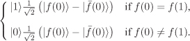
Now, if we measure the input bit, we deterministically get the integer 1 or 0 according as whether f is constant or not respectively. That’s it!

Deutsch’s algorithm solved a rather artificial problem, but it opened up the possibilities of exploring a new paradigm of computation. Till date, (good) quantum algorithms are known for many interesting computational problems. In the rest of this chapter, we concentrate on some of the quantum algorithms that have an impact in cryptology.

Exercise Set 8.2

8.1	Let S be a finite set and let l2(S) denote the set of all functions . Show that l2(S) is a Hilbert space under the inner product Let , where δx(y) is 1 if y = x, and is 0 otherwise. Show that B is an orthonormal basis of l2(S).
8.2	Show that the vectors and form an orthonormal -basis of .
8.3	Show that is an entangled state of a 2-bit quantum register.
8.4	Prove the following assertions. The matrix is unitary. A unitary matrix preserves inner product, that is, if U is an m × m unitary matrix and |ψ〉, , then . The determinant of a unitary matrix has absolute value 1. Every eigen value of a unitary matrix has absolute value 1. An m × m matrix A is unitary if and only if the columns of A constitute an orthonormal basis of (over ).
8.5	Show that the following operators are unitary on a qubit. Also construct the corresponding transformation matrices. Identity operator I|0〉 = |0〉, I|1〉 = |1〉. Exchange operator X|0〉 = |1〉, X|1〉 = |0〉. Z operator Z|0〉 = |0〉, Z|1〉 = –|1〉. Hadamard operator . Deduce the following identities: Let . Show that defines a unitary operator on a qubit and that , where the last X is the matrix of the exchange operator.
8.6	Let A be an n-bit quantum register. Let us plan to number the bits of A as 1, . . . , n from left to right. One can apply the operators like X, Z, H of Exercise 8.5 on each individual bit of A. A qubit operation B applied on bit i of A will be denoted by Bi. Let Sij be the operator that swaps bit i with bit j. Show that Let C be the reversible XOR operation (also called the controlled-NOT operation) on a two-bit register A = (A1A2), that is, C|xy〉 = |x〉|x ⊕ y〉. Show that C can be realized as
8.7	Suppose that whenever you switch on your quantum computer, every bit in its registers is initialized to the state |0〉. Describe how you can use the operators I, X, Z and H defined in Exercise 8.5, in order to change the state of a qubit from |0〉 to the following: |1〉 –|1〉
8.8	Let A be an n-bit quantum register at the state |0|〉n. Show that the application of the Hadamard transform individually to each bit of A transforms A to the state . This is precisely the state of A in which all of the 2n possible outcomes in a measurement of A are equally likely. What happens if we apply H a second time individually to each bit of A, that is, what is H1H2 · · · Hn|ψ〉, where Hi denotes the Hadamard transform on the i-th bit of A?
8.9	We know that any arithmetic or Boolean operation can be implemented using AND and NOT gates. This exercise suggests a reversible way to implement these operations. The Toffoli gate is a function T : {0, 1}3 → {0, 1}3 that maps (x, y, z) ↦ (x, y, z ⊕ xy), where ⊕ means XOR, and xy means AND of x and y. Thus, T flips the third bit, if and only if the first two bits are both 1. Show that T is a unitary transformation on a 3-bit quantum register. What is the inverse of T? Use T to realize the Boolean AND and NOT operations.