
2.5. Integers
The set ![]() of integers is the main object of study in this section. We use many results from previous sections to derive properties of integers. Recall that
of integers is the main object of study in this section. We use many results from previous sections to derive properties of integers. Recall that ![]() is a PID and hence a UFD.
is a PID and hence a UFD.
2.5.1. Divisibility
The notions of divisibility, prime and relatively prime integers, gcd and lcm of integers are essentially the same as discussed in connection with a PID or a UFD. We avoid repeating the definitions here, but concentrate on other useful properties of integers, not covered so far. We only mention that whenever we talk about a prime integer, or the gcd or lcm of two or more integers, we will usually refer to a non-negative integer. This convention makes primes, gcds and lcms unique.
Theorem 2.12.
|
There are infinitely many prime integers. Proof Let |
Theorem 2.13.
The integers q and r in the above theorem are respectively called the quotient and the remainder of Euclidean division of a by b and are denoted respectively by a quot b and a rem b. Do not confuse Euclidean division with the division (that is, the inverse of multiplication) of the ring ![]() . Euclidean division is the basis of the Euclidean gcd algorithm. More specifically:
. Euclidean division is the basis of the Euclidean gcd algorithm. More specifically:
Proposition 2.15.
|
For integers a, b with b ≠ 0, let r be the remainder of Euclidean division of a by b. Then gcd(a, b) = gcd(b, r). Proof Clearly, 〈a〉 + 〈b〉 = 〈r〉 + 〈b〉. Now use Proposition 2.14. |
Proposition 2.16.
|
Let a and b be two integers, not both zero, and let d be the (positive) gcd of a and b. Then there are integers u and v such that d = ua + vb. (Such an equality is called a Bézout relation.) Furthermore, if a and b are both non-zero and (|a|, |b|) ≠ (1, 1), then u and v can be so chosen that |u| < |b| and |v| < |a|. Proof The existence of u and v follows immediately from Proposition 2.14. If a = qb, then u = 0 and v = 1 is a suitable choice. So assume that a b and b a, in which case d < |a| and d < |b|. We may assume, without loss of generality, that a and b are positive. First note that if (u, v) satisfies the Bézout relation, then for any |
The notions of the gcd and of the Bézout relation can be generalized to any finite number of integers a1, . . . , an as
gcd(a1, . . . , an) = gcd(· · · (gcd(gcd(a1, a2), a3) · · ·), an) = u1a1 + · · · + unan
for some integers u1, . . . , un (provided that all the gcds mentioned are defined).
2.5.2. Congruences
Since ![]() is a PID, congruence modulo a non-zero ideal of
is a PID, congruence modulo a non-zero ideal of ![]() can be rephrased in terms of congruence modulo a positive integer as follows.
can be rephrased in terms of congruence modulo a positive integer as follows.
Definition 2.27.
|
Let |
By an abuse of notation, we often denote the equivalence class [a] of ![]() simply by a. The following are some basic properties of congruent integers.
simply by a. The following are some basic properties of congruent integers.
Proposition 2.17.
|
Let
Proof (1) and (2) follow from the consideration of the quotient ring |
Let ![]() with gcd(ni, nj) = 1 for i ≠ j. Then lcm(n1, . . . , nr) = n1 · · · nr, and by the Chinese remainder theorem (Theorem 2.10), we have
with gcd(ni, nj) = 1 for i ≠ j. Then lcm(n1, . . . , nr) = n1 · · · nr, and by the Chinese remainder theorem (Theorem 2.10), we have
![]()
This implies that, given integers a1, . . . , ar, there exists an integer x unique modulo n1 · · · nr such that x satisfies the following congruences simultaneously:
| x | ≡ | a1 (mod n1) |
| x | ≡ | a2 (mod n2) |
| ⋮ | ||
| x | ≡ | ar (mod nr) |
We now give a procedure for constructing the integer x explicitly. Define N := n1 · · · nr and Ni := N/ni for 1 ≤ i ≤ r. Then for each i we have gcd(ni, Ni) = 1 and, therefore, there are integers ui and vi with uini + viNi = 1. Then ![]() (mod N) is the desired solution.
(mod N) is the desired solution.
Let ![]() . We now study the multiplicative group
. We now study the multiplicative group ![]() of the ring
of the ring ![]() . We say that an integer
. We say that an integer ![]() has a multiplicative inverse modulo n, if
has a multiplicative inverse modulo n, if ![]() , or, equivalently, if there is an integer b with ab ≡ 1 (mod n). The following proposition is an important characterization of the elements of
, or, equivalently, if there is an integer b with ab ≡ 1 (mod n). The following proposition is an important characterization of the elements of ![]() .
.
Proposition 2.18.
|
(The equivalence class of) an integer a belongs to Proof [if] By Proposition 2.16, there exist integers u and v such that ua + vn = 1. But then ua ≡ 1 (mod n). [only if] For some integers u and v, we have ua + vn = 1, which implies that the gcd of a and n divides 1 and hence is equal to 1. |
Definition 2.28.
|
The cardinality of |
The following two theorems are immediate consequences of Proposition 2.4.
Theorem 2.14. Euler’s theorem
|
Let aφ(n) ≡ 1 (mod n). |
Theorem 2.15. Fermat’s little theorem
|
Let p be a prime and ap–1 ≡ 1 (mod p). For any integer |
Theorem 2.16. Wilson’s theorem
|
For every prime p, we have (p – 1)! ≡ –1 (mod p). Proof The result holds for p = 2. So assume that p is an odd prime. Since Equation 2.1
Looking at the constant terms in two sides proves Wilson’s theorem. |
The structure of the group ![]() ,
, ![]() , can be easily deduced from Fermat’s little theorem. This gives us the following important result.
, can be easily deduced from Fermat’s little theorem. This gives us the following important result.
Proposition 2.19.
|
For a prime p, the group Proof For every divisor d of p –1, we have Xp–1–1 = (Xd–1)f(X) for some |
Euler’s totient function plays an extremely important role in number theory (and cryptology). We now describe a method for computing it.
Lemma 2.2.
Lemma 2.3.
|
If p is a prime and Proof Integers between 0 and pe – 1, which are relatively prime to pe are precisely those that are not multiples of p. |
Proposition 2.20.
|
Let
Proof Immediate from Lemmas 2.2 and 2.3. |
By Proposition 2.18, the linear congruence ax ≡ 1 (mod n) is solvable for x if and only if gcd(a, n) = 1. In such a case, the solution is unique modulo n. Now, let us concentrate on the solutions of the general linear congruence:
ax ≡ b (mod n).
Theorem 2.17 characterizes the solutions of this congruence.
Theorem 2.17.
|
Let d := gcd(a, n). Then the congruence ax ≡ b (mod n) is solvable for x if and only if d|b. A solution of the congruence, if existent, is unique modulo n/d. Proof [if] By Proposition 2.17, (a/d)x ≡ b/d (mod n/d). Since gcd(a/d, n/d) = 1, the congruence (a/d)x′ ≡ 1 (mod n/d) is solvable for x′. Then a solution for x is x ≡ (b/d)x′ (mod n/d). [only if] There exists an integer k such that ax + kn = b. This shows that d|b. To prove the uniqueness let x and x′ be two integers satisfying the given congruence. But then a(x – x′) ≡ 0 (mod n), that is, (a/d)(x – x′) ≡ 0 (mod n/d), that is, x – x′ ≡ 0 (mod n/d), since gcd(a/d, n/d) = 1. |
The last theorem implies that if d|b, then the congruence ax ≡ b (mod n) has d solutions modulo n. These solutions are given by ξ + r(n/d), r = 0, . . . , d – 1, where ξ is the solution modulo n/d of the congruence (a/d)ξ ≡ b/d (mod n/d).
2.5.3. Quadratic Residues
In this section, we consider quadratic congruences, that is, congruences of the form ax2+bx+c ≡ 0 (mod n). We start with the simple case ![]() . We assume further that p is odd, so that 2 has a multiplicative inverse mod p. Since we are considering quadratic equations, we are interested only in those integers a for which gcd(a, p) = 1. In that case, a also has a multiplicative inverse mod p and the above congruence can be written as y2 ≡ α (mod p), where y ≡ x + b(2a)–1 (mod p) and α ≡ b2(4a2)–1 – c(a–1) (mod p). This motivates us to provide Definition 2.29.
. We assume further that p is odd, so that 2 has a multiplicative inverse mod p. Since we are considering quadratic equations, we are interested only in those integers a for which gcd(a, p) = 1. In that case, a also has a multiplicative inverse mod p and the above congruence can be written as y2 ≡ α (mod p), where y ≡ x + b(2a)–1 (mod p) and α ≡ b2(4a2)–1 – c(a–1) (mod p). This motivates us to provide Definition 2.29.
Definition 2.29.
If a is a quadratic residue modulo an odd prime p, then the equation x2 ≡ a (mod p) has exactly two solutions. If ξ is one solution, the other solution is p – ξ. It is, therefore, evident that there are exactly (p – 1)/2 quadratic residues and exactly (p – 1)/2 quadratic non-residues modulo p. For example, the quadratic residues modulo p = 11 are 1 = 12 = 102, 3 = 52 = 62, 4 = 22 = 92, 5 = 42 = 72 and 9 = 32 = 82. The quadratic non-residues modulo 11 are, therefore, 2, 6, 7, 8 and 10. We treat 0 neither as a quadratic residue nor as a quadratic non-residue.
Definition 2.30.
|
Let p be an odd prime and a an integer with gcd(a, p) = 1. The Legendre symbol
|
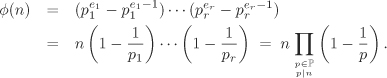
Proposition 2.21.
|
Let p be an odd prime and a and b integers coprime to p.
Proof If a is a quadratic residue modulo p, then a ≡ b2 (mod p) for some integer b (coprime to p) and by Fermat’s little theorem we have a(p–1)/2 ≡ bp–1 ≡ 1 (mod p). Conversely, the polynomial Xp–1 – 1 = (X(p–1)/2 – 1)(X(p–1)/2 + 1) has p – 1 (distinct) roots mod p (again by Fermat’s little theorem). We have seen that no quadratic residues are roots of X(p–1)/2 + 1. Since |
Euler’s criterion gives us a nice way to check if a given integer is a quadratic residue modulo an odd prime. While this is much faster than the brute-force strategy of enumerating all the quadratic residues, it is still not the best solution, because it involves a modular exponentiation. We can, however, employ a gcd-like procedure for a faster computation. The development of this method demands further results which are otherwise interesting in themselves as well. The first important result is known as the law of quadratic reciprocity (Theorem 2.18 below). Gauss was the first to prove it and he deemed the result so important that he gave eight proofs for it. At present about two hundred published proofs of this law exist in the literature. We go in the classical way, that is, the Gaussian way, because the proof, though somewhat long, is elementary.
Lemma 2.4. Gauss
|
Let p be an odd prime and a an integer with gcd(a, p) = 1. Let us denote t := (p – 1)/2. For an integer i, let ri be the unique integer with ri ≡ ia (mod p) and –t ≤ ri ≤ t. Let n be the number of i, 1 ≤ i ≤ t, for which ri is negative. Then Proof It is easy to check that ri ≢ ±rj (mod p) for all i ≠ j with 1 ≤ i, j ≤ t. Thus |ri|, i = 1, . . . , t, are precisely (a permuted version of) the integers 1, . . . , t. Thus |
Definition 2.31.
|
Let |
Corollary 2.7.
|
With the notations of Lemma 2.4 we have Proof Since If a is odd, p + a is even. Also 4 is a quadratic residue modulo p. So |
Theorem 2.18. Law of quadratic reciprocity
|
Let p and q be distinct odd primes. Then Proof By Corollary 2.7, |
To demonstrate how we can use the results deduced so far, let us compute ![]() . Since 360 = 23 · 32 · 5, we have
. Since 360 = 23 · 32 · 5, we have
Thus 360 is a quadratic residue modulo 997. The apparent attractiveness of this method is beset by the fact that it demands the factorization of several integers and as such does not lead to a practical algorithm. We indeed need further machinery in order to have an efficient algorithm. First, we define a generalization of the Legendre symbol.
Definition 2.32.
|
Let a, b be integers with b > 0 and odd. We define the Jacobi symbol
where, in the last case, p1, . . . , pt are all the prime factors of b (not necessarily all distinct). |

Note that if ![]() , then a is not a quadratic residue mod b. However, the converse is not always true, that is,
, then a is not a quadratic residue mod b. However, the converse is not always true, that is, ![]() does not necessarily imply that a is a quadratic residue modulo b (Example: a = 2 and b = 9). Of course, if b is an odd prime and if gcd(a, b) = 1, the Legendre and Jacobi symbols
does not necessarily imply that a is a quadratic residue modulo b (Example: a = 2 and b = 9). Of course, if b is an odd prime and if gcd(a, b) = 1, the Legendre and Jacobi symbols ![]() correspond to the same value and meaning.
correspond to the same value and meaning.
The Jacobi symbol enjoys many properties similar to the Legendre symbol.
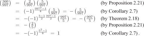
Proposition 2.22.
|
For integers a, a′ and positive odd integers b, b′, we have:
Proof Immediate from the definition and Proposition 2.21. |
Theorem 2.19.
Proof
|
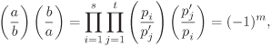

Now, we can calculate ![]() without factoring as follows.
without factoring as follows.
2.5.4. Some Assorted Topics
So far, we have studied some elementary properties of integers. Number theory is, however, one of the oldest and widest branches of mathematics. Various complex-analytic and algebraic tools have been employed to derive more complicated properties of integers. In Section 2.13, we give a short introductory exposition to algebraic number theory. Here, we mention a collection of useful results from analytic number theory. The proofs of these analytic results would lead us too far away and hence are omitted here. Inquisitive (and/or cynical) readers may consult textbooks on analytic number theory for the details missing here.
The prime number theorem
The famous prime number theorem gives an asymptotic estimate of the density of primes smaller than or equal to a positive real number. Gauss conjectured this result in 1791. Many mathematicians tried to prove it during the 19th century and came up with partial results. Riemann made reasonable progress towards proving the theorem, but could not furnish a complete proof before he died in 1866. It is interesting to mention here that a good portion of the theory of analytic functions (also called holomorphic functions) in complex analysis was developed during these attempts to prove the prime number theorem. The first complete proof of the theorem (based mostly on the ideas of Riemann and Chebyshev) was given independently by the French mathematician Hadamard and by the Belgian mathematician de la Vallée Poussin in 1896. Their proof is regarded as one of the major achievements of modern mathematics. People started believing that any proof of the prime number theorem has to be analytic. Erdös and Selberg destroyed this belief by independently providing the first elementary proof of the theorem in 1949. Here (and elsewhere in mathematics), the adjective elementary refers to something which does not depend on results from analysis or algebra. Caution: Elementary is not synonymous with easy !
Theorem 2.20. Prime Number Theorem
|
Let π(x) denote the number of primes less than or equal to a real number x > 0. As x → ∞ we have π(x) → x/ln x (that is, the ratio π(x)/(x/ln x) → 1). In particular, for |
Though the prime number theorem provides an asymptotic estimate (that is, one for x → ∞), for finite values of x (for example, for the values of x in the cryptographic range) it does give good approximations for π(x). Table 2.1 lists π(x) against the rounded values of x/ ln x for x equal to small powers of 10.
| x | π(x) | x/ ln x | x/(ln x – 1) | Li(x) |
|---|---|---|---|---|
| 103 | 168 | 145 | 169 | 178 |
| 104 | 1229 | 1086 | 1218 | 1246 |
| 105 | 9592 | 8686 | 9512 | 9630 |
| 106 | 78,498 | 72,382 | 78,030 | 78,628 |
| 107 | 664,579 | 620,421 | 661,458 | 664,918 |
| 108 | 5,761,455 | 5,428,681 | 5,740,304 | 5,762,209 |
Given the prime number theorem it follows that π(x) approaches x/(ln x – ξ) for any real ξ. It turns out that ξ = 1 is the best choice. Gauss’ Li function is also an asymptotic estimate for π(x), where for real x > 0 one defines:
![]()
Gauss conjectured that Li(x) asymptotically equals π(x). The prime number theorem is, in fact, equivalent to this conjecture. Furthermore, de la Vallée Poussin proved that Li(x) is a better approximation to π(x) than x/(ln x – ξ) for any real ξ. Table 2.1 also lists x/(ln x – 1) and Li(x) against the actual values of π(x).
The asymptotic formula ![]() does not rule out the possibility that the error π(x)–(x/ ln x) tends to zero as x → ∞. It has been shown by Dusart [83] that (x/ ln x) – 0.992(x/ ln2 x) ≤ π(x) ≤ (x/ ln x) + 1.2762(x/ ln2 x) for all x > 598.
does not rule out the possibility that the error π(x)–(x/ ln x) tends to zero as x → ∞. It has been shown by Dusart [83] that (x/ ln x) – 0.992(x/ ln2 x) ≤ π(x) ≤ (x/ ln x) + 1.2762(x/ ln2 x) for all x > 598.
Density of smooth integers
Integers having only small prime divisors play an interesting role in cryptography and in number theory in general.
Definition 2.33.
|
Let |
The following theorem gives an asymptotic estimate for ψ(x, y).
Theorem 2.21.
|
Let x, ψ(x, y) → u–u+o(u) = e–[(1+o(1))u ln u]. |
In Theorem 2.21, the notation g(u) = o(f(u)) implies that the ratio g(u)/f(u) tends to 0 as u approaches ∞. See Definition 3.1 for more details. An interesting special case of the formula for ψ(x, y) will be used quite often in this book and is given as Corollary 4.1 in Chapter 4.
Like the prime number theorem, Theorem 2.21 gives only asymptotic estimates, but is indeed a good approximation for finite values of x, y and u (that is, for the values of practical interest). The most important implication of this theorem is that the density of y-smooth integers in the set {1, . . . , x} is a very sensitive function of u = ln x/ ln y and decreases very rapidly as x increases. For example, if y = 15,485,863, the millionth prime, then a random integer ≤ 2250 is y-smooth with probability approximately 2.12 × 10⁻¹¹, whereas a random integer ≤ 2500 is y-smooth with probability approximately 2.23 × 10⁻²⁸. (These figures are computed neglecting the o(u) term in the expression of ψ(x, y).) In other words, smaller integers have higher probability of being smooth (that is, y-smooth for a given y).
The extended Riemann hypothesis
The Riemann hypothesis (RH) is one of the deepest unsolved problems in mathematics. An extended version of this hypothesis has important bearings on the solvability of certain computational problems in polynomial time.
Definition 2.34.
|
The Euler zeta function ζ(s) is defined for a complex variable s with Re s ≥ 1 as
The reader may already be familiar with the results: ζ(1) = ∞, ζ(2) = π2/6 and ζ(4) = π4/90. Riemann (analytically) extended the Euler Zeta function for all complex values of s (except at s = 1, where the function has a simple pole). This extended function, called the Riemann zeta function, is known to have zeros at s = –2, –4, –6, . . . . These are called the trivial zeros of ζ(s). It can be proved that all non-trivial zeros of ζ(s) must lie in the so-called critical strip : 0 ≤ Re s ≤ 1, and are symmetric about the critical line: Re s = 1/2. |
Conjecture 2.1. Riemann hypothesis (RH)
In 1900, Hilbert asserted that proving or disproving the RH is one of the most important problems confronting 20th century mathematicians. The problem continues to remain so even to the 21st century mathematicians.
In 1901, von Koch proved that the RH is equivalent to the formula:
Conjecture 2.2. An equivalent form of the Riemann hypothesis
|
π(x) = Li(x) + O(x1/2 ln x) |
Here the order notation f(x) = O(g(x)) means that |f(x)/g(x)| is less than a constant for all sufficiently large x (See Definition 3.1).
Hadamard and de la Vallée Poussin proved that
![]()
for some positive constant α. While this estimate was sufficient to prove the prime number theorem, the tighter bound of Conjecture 2.2 continues to remain unproved.
Theorem 2.22. Dirichlet’s theorem on primes in arithmetic progression
|
Let a, |
Dirichlet’s theorem is a powerful generalization of Theorem 2.12 (which corresponds to a = b = 1). One can accordingly generalize the notation π(x) as follows:
Definition 2.35.
|
Let a, |
The prime number theorem gives the estimate:
![]()
where φ is Euler’s totient function. The RH now generalizes to:
Conjecture 2.3. Extended Riemann hypothesis (ERH)
|
For a,
|
Some authors use the expression Generalized Riemann hypothesis (GRH) in place of ERH. Taking b = 1 demonstrates that the ERH implies the RH. The ERH also implies the following:
Conjecture 2.4.
|
The smallest positive quadratic non-residue modulo a prime p is < 2 ln2 p. |
Exercise Set 2.5
| 2.35 |
|
| 2.36 | Let
|
| 2.37 | Show that for any |
| 2.38 |
|
| 2.39 | Let n ≥ 2 be a natural number. A complete residue system modulo n is a set of n integers a1, . . . , an such that ai ≢ aj (mod n) for i ≠ j. Similarly, a reduced residue system modulo n is a set of φ(n) integers b1, . . . , bφ(n) such that gcd(bi, n) = 1 for all i = 1, . . . , φ(n) and bi ≢ bj (mod n) for i ≠ j. Show that:
|
| 2.40 | Prove that the decimal expansion of any rational number a/b is recurring, that is, (eventually) periodic. (A terminating expansion may be viewed as one with recurring 0.) [H] |
| 2.41 | Let p be an odd prime. Show that the congruence x2 ≡ –1 (mod p) is solvable if and only if p ≡ 1 (mod 4). [H] |
| 2.42 | Let |
| 2.43 | For |
| 2.44 | Let n > 2 and gcd(a, n) = 1. Let h be the multiplicative order of a modulo n (that is, in the group
|
| 2.45 | Device a criterion for the solvability of ax2 + bx + c ≡ 0 (mod p), where p is an odd prime and gcd(a, p) = 1. [H] |
| 2.46 | Let p be a prime and |
| 2.47 | Let G be a finite cyclic group of cardinality n. Show that |
| 2.48 | Let m, |
| 2.49 | In this exercise, we investigate which of the groups
|
| 2.50 | Show that the multiplicative group |