**2.13. Number Fields

In this section, we develop the theory of number fields and rings. Our aim is to make accessible to the readers the working of the cryptanalytic algorithms based on number field sieves.

2.13.1. Some Commutative Algebra

Commutative algebra is the study of commutative rings with identity (rings by our definition). Modern number theory and geometry are based on results from this area of mathematics. Here we give a brief sketch of some commutative algebra tools that we need for developing the theory of number fields.

Ideal arithmetic

We start with some basic operations on ideals (cf. Example 2.7, Definition 2.23).

Definition 2.92.

Let A be a ring and let , , be a family (not necessarily finite) of ideals in A. The set-theoretic intersection is evidently an ideal in A. The sum of the family is the ideal Two ideals and of A are said to be relatively prime or coprime, if , or equivalently if there exist and with a + b = 1. If I = {1, 2, . . . , n} is finite, the product is the ideal generated by all elements of the form x1x2 . . . xn with for all i = 1, . . . , n. We have: If , the product is denoted as . The empty product of ideals is conventionally taken to be the unit ideal A. If is the principal ideal 〈a〉, then .

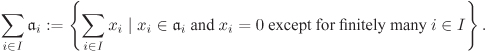
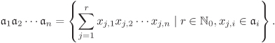
One can readily check that the operations intersection, sum and product on ideals in a ring are associative and commutative.

Commutative algebra extensively uses the theory of prime and maximal ideals (Definition 2.19, Proposition 2.9, Corollary 2.2 and Exercise 2.23). The set of all prime ideals in A is called the (prime) spectrum of A and is denoted by Spec A. The set of all maximal ideals of A is called the maximal spectrum of A and denoted by Spm A. We have Spm A ⊆ Spec A. These two sets play an extremely useful role for the study of the ring A. If A is non-zero, both these sets are non-empty.

Localization

The concept of formation of fractions of integers to give the rationals can be applied in a more general setting. Instead of having any non-zero element in the denominator of a fraction we may allow only elements from a specific subset. All we require to make the collection of fractions a ring is that the allowed denominators should be closed under multiplication.

Definition 2.93.

Let A be a ring. A non-empty subset S of A is called multiplicatively closed or simply multiplicative, if and for any s, we have .

Example 2.25.

For a non-zero ring A, the subset A {0} is multiplicatively closed, if and only if A is an integral domain. For a general non-zero ring A, the set of all elements such that a is not a zero-divisor is a multiplicative subset of A. Let A be a ring and a a proper ideal of A. The set is multiplicatively closed, if and only if is a prime ideal of A. For a ring A and an element , the set {1, f, f2, f3, . . .} ⊆ A is multiplicatively closed.

Let A be a ring and S a multiplicative subset of A. We define a relation ~ on A × S as: (a, s) ~ (b, t) if and only if u(at – bs) = 0 for some . (If A is an integral domain, one may take u = 1 in the definition of ~.) It is easy to check that ~ is an equivalence relation on A × S. The set of equivalence classes of A × S under ~ is denoted by S^–1A, whereas the equivalence class of is denoted as a/s. For a/s, , define (a/s) + (b/t) := (at + bs)/(st) and (a/s)(b/t) := (ab)/(st). It is easy to check that these operations are well-defined and make S^–1 A a ring with identity 1/1, in which each s/1, , is invertible. There is a canonical ring homomorphism taking a ↦ a/1. In general, is not injective. However, if A is an integral domain and 0 ∉ S, then the injectivity of can be proved easily and we say that the ring A is canonically embedded in the ring S^–1A.

Definition 2.94.

Let A be a ring and S a multiplicative subset of A. The ring S–1A constructed as above is called the localization of A away from S or the ring of fractions of A with respect to S.

Example 2.26.

Let A be an integral domain and let S = A {0}. Then S–1A is called the quotient field or the field of fractions of A and is denoted as Q(A). If A is already a field, then Q(A) ≅ A. Other examples include and Q(K[X]) = K(X), K a field, where K(X) denotes the field of rational functions over K in one indeterminate X. More generally, if A is any ring and S is the set of all non-zero-divisors of A, then S–1A is called the total quotient ring of A and is again denoted by Q(A). It is, in general, not a field. If A is an integral domain, then S = A {0} and the usage of Q(A) remains consistent. Let A be a ring, a prime ideal of A and . Then S–1A is called the localization of A at and is usually denoted by Ap. Let A be a ring, and S = {1, f, f2, f3, . . . }. In this case, S–1A is conventionally denoted by Af.

Integral dependence

The concept of integral dependence generalizes the notion of integers. Recall that for a field extension K ⊆ L, an element is called algebraic over K, if α is a root of a non-zero polynomial . Since K is a field, the polynomial f can be divided by its leading coefficient, giving a monic polynomial in K[X] of which α is a root. However, if K is not a field, division by the leading coefficient is not always permissible. So we require the minimal polynomial to be monic in order to define a special class of objects.

Definition 2.95.

Let A ⊆ B be an extension of rings. An element is said to be integral over A, if α satisfies[15] (that is, is a root of) a monic (and hence non-zero) polynomial . An equation of the form f(α) = 0, monic, is called an equation of integral dependence of α over A. [15] Strictly speaking, α being a root of f(X) is equivalent to α satisfying the polynomial equation f(α) = 0. Often the term equation is dropped in this context—a harmless colloquial contraction.

Example 2.27.

If both A and B are fields, the concepts of integral and algebraic elements are the same. (See the argument preceding Definition 2.95.) Take and and let , gcd(a, b) = 1, be integral over . Let (a/b)n + αn–1(a/b)n–1 + · · · + α1(a/b) + α0, , be an equation of integral dependence of a/b over . Multiplication by bn gives an = –b(αn–1an–1 + · · · + α1abn–2 + α0bn–1), that is, b|an. Since gcd(a, b) = 1, this forces b = ±1, that is, . This is, in general, true for any UFD A and its field of fractions B = Q(A) (See Exercise 2.131). Every element is integral over A, since it satisfies the monic polynomial .

Now let A ⊆ B be an extension of rings and let C consist of all the elements of B that are integral over A. Clearly, A ⊆ C ⊆ B. It turns out that C is again a ring. This result is not at all immediate from the definition of integral elements. We prove this by using the following lemma which generalizes Theorem 2.33.

Lemma 2.11.

For a ring extension A ⊆ B and for , the following conditions are equivalent: α is integral over A. A[α] is a finitely generated A-module. A[α] ⊆ C for some subring C of B with C being a finitely generated A-module. Proof [(a)⇒(b)] Let αn + an–1αn–1 + · · · + a1α + a0 = 0, , be an equation of integral dependence of α over A. is generated as an A-module by 1, α, α2, . . . . In order to show that only the elements 1, α, . . . , αn–1 generate A[α] as an A-module, it is sufficient to show that each αk, , is an A-linear combination of 1, α, . . . , αn–1. We proceed by induction on k. The assertion certainly holds for k = 0, . . . , n – 1, whereas for k ≥ n we write αk = –(an–1αk–1 + · · · + a1αk–n+1 + a0αk–n), whence induction completes the proof. [(b)⇒(c)] Take C := A[α]. [(c)⇒(a)] Let generate C as an A-module. Since A[α] ⊆ C and, in particular, , for all i = 1, . . . , n we can write for some . Let denote the matrix (αδij – aij)1≤i,j≤n, where δij is the Kronecker delta. Then . Multiplication (on the left) by the adjoint of shows that for all i = 1, . . . , n. Since , we have for some , so that (det ) · 1 = 0, that is, det . But det is a monic polynomial in α of degree n and with coefficients from A.

Proposition 2.42.

For an extension A ⊆ B of rings, the set is a subring of B containing A. Proof Clearly, A ⊆ C ⊆ B as sets. To show that C is a ring let α, . By Condition (b) of Lemma 2.11, A[α] is a finitely generated A-module. Now β, being integral over A, is also integral over A[α]; so again by Lemma 2.11(b), A[α][β] is a finitely generated A[α]-module. It is then easy to check that A[α, β] = A[α][β] is a finitely generated A-module. Since α ± β and αβ are in A[α, β], by Lemma 2.11(c), these elements are integral over A, that is, belong to C. Thus C is a ring.

Definition 2.96.

The ring C of Proposition 2.42 is called the integral closure of A in B. A is called integrally closed in B, if C = A. On the other hand, if C = B, we say that B is an integral extension of A or that B is integral over A. An integral domain A is called integrally closed (without specific mention of the ring in which it is so), if A is integrally closed in its quotient field Q(A). An integrally closed integral domain is called a normal domain (ND).

Example 2.28.

(or more generally any UFD) is a normal domain. is not integrally closed in or , since, for example, is integral over . The integral closure of in is denoted by . Elements of are called algebraic integers (See Exercise 2.60).

Noetherian rings

Recall that a PID is a ring (integral domain) in which every ideal is principal, that is, generated by a single element. We now want to be a bit more general and demand every ideal to be finitely generated. If a ring meets our demand, we call it a Noetherian ring. These rings are named after Emmy Noether (1882–1935) who was one of the most celebrated lady mathematicians of all ages and whose work on Noetherian rings has been very fundamental and deep in the branch of algebra. Emmy’s father Max Noether (1844 –1921) was also an eminent mathematician.

Definition 2.97.

Let A be a ring and let be an ascending chain of ideals of A. This chain is called stationary, if there is an such that . The ring A is said to satisfy the ascending chain condition or the ACC, if every ascending chain of ideals in A is stationary, or in other words, if there does not exist any infinite strictly ascending chain of ideals in A.

Proposition 2.43.

For a ring A, the following conditions are equivalent: Every ideal of A is finitely generated. A satisfies the ascending chain condition. Every non-empty set of ideals of A contains a maximal element. Proof [(a)⇒(b)] Let be an ascending chain of ideals of A. Consider the ideal which is finitely generated by hypothesis. Let a1, . . . , ar be a set of generators of . Each , that is, there exists such that and hence for every n ≥ mi. Take m := max(m1, . . . , mr). For every n ≥ m, we have a , that is, . [(b)⇒(c)] Let S be a non-empty set of ideals of A. Order S by inclusion. The ACC implies that every chain in S has an upper bound in S. By Zorn’s lemma, S has a maximal element. [(c)⇒(a)] Let be an ideal of A. Consider the set S of all finitely generated ideals of A contained in . S is non-empty, since it contains the zero ideal. By condition (c), S has a maximal element, say, . If , take . Then is finitely generated (since is so), properly contains and is contained in . This contradicts the maximality of in S. Thus we must have , that is, is finitely generated.

Definition 2.98.

A ring A is called Noetherian, if A satisfies (one and hence all of) the equivalent conditions of Proposition 2.43.

Example 2.29.

All PIDs are Noetherian, since principal ideals are obviously finitely generated. In particular, and K[X] (K a field) are Noetherian. If A is Noetherian and an ideal of A, then is Noetherian, since the ideals of are in one-to-one inclusion-preserving correspondence with the ideals of A containing a and hence satisfy the ACC. Let A be a Noetherian ring and S a multiplicative subset of A. Then the localization B := S–1A is also Noetherian. To prove this fact let be an ideal in B. One can show that for some ideal of A. Since A is Noetherian, is finitely generated, say, . It is now (almost) obvious that is generated by a1/1, . . . , ar/1. A particular case: If A is Noetherian and a prime ideal of A, then the localization is also Noetherian. The ring of polynomials with infinitely many indeterminates X1, X2, X3, . . . is not Noetherian. This is because the ideal 〈X1, X2, X3, . . .〉 = AX1 + AX2 + AX3 + · · · is not finitely generated, or alternatively because we have the infinite strictly ascending chain of ideals: 〈X1〉  〈X1, X2〉  〈X1, X2, X3〉  · · ·, or because the set S := {〈X1〉, 〈X1, X2〉, 〈X1, X2, X3〉, . . .} of ideals in A does not contain a maximal element.

We have seen that if A is a PID, the polynomial ring A[X] need not be a PID. However, the property of being Noetherian is preserved during the passage from A to A[X] (Theorem 2.8).

Dedekind domains

A class of rings proves to be vital in the study of number fields:

Definition 2.99.

An integral domain A is called a Dedekind domain, if it satisfies all of the following three conditions: A is Noetherian. Every non-zero prime ideal of A is maximal. A is integrally closed (in its quotient field K := Q(A)).

2.13.2. Number Fields and Rings

After much ado we are finally in a position to define the basic objects of study in this section.

Definition 2.100.

A number field K is defined to be a finite (and hence algebraic) extension of the field of rational numbers. Clearly, . The extension degree is called the degree of the number field K and is finite by definition.

Note that there exist considerable controversies among mathematicians in accepting this definition of number fields. Some insist that any field K satisfying should be called a number field. Some others restrict the definition by demanding that one must have K algebraic over ; however, fields K with infinite extension degree are allowed. We restrict the definition further by imposing the condition that has to be finite. Our restricted definition is seemingly the most widely accepted one. In this book, we study only the number fields of Definition 2.100 and accepting this definition would at the minimum save us from writing huge expressions like “(algebraic) number fields of finite extension degree over ” to denote number fields.

For number fields, the notion of integral closure leads to the following definition.

Definition 2.101.

A number field K contains and hence . The integral closure of in K is called the ring of integers of K and is denoted by . ( is the Gothic O.) Clearly, and is an integral domain. We also have , where is the subset of comprising all algebraic integers. A number ring is a ring which is (isomorphic to) the ring of integers of a number field.

By Example 2.27(2), the ring of integers of the number field is , that is, . It is, therefore, customary to call the elements of rational integers. Since is naturally embedded in for any number field K, it is important to notice the distinction between the integers of K (that is, the elements of ) and the rational integers of K (that is, the images of the canonical inclusion ).

Some simple properties of number rings are listed below.

Proposition 2.44.

For a number field K, we have: . For , there exists a rational integer such that . In particular, the quotient field of is K. is integrally closed in , that is, is a normal domain. Proof (1) follows immediately from Example 2.27(2), (2) follows from Exercise 2.60, and (3) follows from Exercise 2.126(b).

Let K be a number field of degree d. By Corollary 2.13, K is a simple extension of , that is, there exists an element with a minimal polynomial f(X) over such that deg and . The field K is a -vector space of dimension d with basis 1, α, . . . , α^d–1. There exists a nonzero integer a such that is an algebraic integer and we continue to have . Thus, without loss of generality, we may take α to be an algebraic integer. In this case, the -basis 1, α, . . . , α^d–1 of K consists only of algebraic integers.

Conversely, let be an irreducible polynomial of degree d ≥ 1. The field is a number field of degree d and the elements of K can be represented by polynomials with rational coefficients and of degrees < d. Arithmetic in K is carried out as the polynomial arithmetic of followed by reduction modulo the defining irreducible polynomial f(X). This gives us an algebraic representation of K independent of any element of K. Now, K can also be viewed as a subfield of and the elements of K can be represented as complex numbers.^[16] A representation with a field isomorphism is called a complex embedding of K in .^[17] Such a representation is not unique as Proposition 2.45 demonstrates.

^[16] A complex number has a representation by a pair (a, b) of real numbers. Here, plays the role of X + 〈X² + 1〉 in . Finally, every real number has a decimal (or binary or hexadecimal or . . .) representation.

^[17] The field is canonically embedded in K. It is evident that the embedding σ : K → K′ fixes element-wise.

Proposition 2.45.

A number field K of degree d ≥ 1 has exactly d distinct complex embeddings. Proof As above we take for some irreducible polynomial of degree d. Since is a perfect field (See Exercise 2.76), the d roots of f(X) are all distinct. For each i = 1, . . . , d, the map sending X + 〈f(X)〉 ↦ αi clearly extends to a field isomorphism . Thus we get d distinct complex embeddings of K in . Now let K′ be a subfield of , such that is a -isomorphism. Let α := σ(X + 〈f(X)〉). Then 0 = σ(0) = σ(f(X + 〈f(X)〉)) = f(σ(X + 〈f(X)〉)) = f(α). Thus α is a root of f, that is, α = αi for some . Since K′ is a field containing and αi and having , it follows that and σ = σi.

This proposition says that the conjugates α₁, . . . , α_d are algebraically indistinguishable. For example, X² + 1 has two roots ±i, where . But it makes little sense to talk about the positive and the negative square roots of –1? They are algebraically indistinguishable and if one calls one of these i, the other one becomes –i.^[18] However, if a representation of is given, we can distinguish between and by associating these quantities with the elements and respectively, where is the positive real square root of 5 and where is the imaginary unit available from the given representation of .

^[18] In a number theory seminar in 1996, Hendrik W. Lenstra, Jr. commented:

Suppose the Martians defined the complex numbers by adjoining a root of –1 they called j. And when the Earth and Martians start talking, they have to translate i to be either j or –j. So we take i to j, because I think that’s what the scientists will decide. ··· But it was later discovered that most Martians are left handed, so the philosophers decide it’s better to send i to –j instead.

It is also quite customary to start with for some algebraic and seek for the complex embeddings of K in . One then considers the minimal polynomial f(X) of α (over ) and proceeds as in the proof of Proposition 2.45 but now defining the map as the unique field isomorphism that fixes and takes α ↦ α_i. If we take α = α₁, then σ₁ is the identity map, whereas σ₂, . . . , σ_d are non-identity field isomorphisms.

The moral of this story is that whether one wants to view the number field K as or as for any is one’s personal choice. In any case, one will be dealing with the same mathematical object and as long as representation issues are not brought into the scene, all these definitions of a number field are absolutely equivalent.

The embeddings need not be all distinct as sets. For example, the two embeddings and of are identical as sets. But the maps x ↦ i and x ↦ –i are distinct (where x := X + 〈X² + 1〉). Thus while specifying a complex embedding of a number field K, it is necessary to mention not only the subfield K′ of isomorphic to K, but also the explicit field isomorphism K → K′.

Definition 2.102.

Let K be a number field of degree d defined by an irreducible polynomial or by any root of f(X). Let r1 be the number of real roots and 2r2 the number of non-real roots of f. (Note that the non-real roots of a real polynomial occur in (complex) conjugates.) By the fundamental theorem of algebra, we have d = r1 + 2r2. For any real root α of f, the complex embedding of K is completely contained in and hence is often called a real embedding of K. On the other hand, for a non-real root β of f the complex embedding of K is called a non-real or a properly complex embedding of K. The pair (r1, r2) is called the signature of the number field K. K has r1 real embeddings and 2r2 properly complex embeddings. If r2 = 0, that is, if all embeddings of K are real, one calls K a totally real number field. On the other hand, if r1 = 0, that is, if all embeddings of K are properly complex, then K is called a totally complex number field.

Example 2.30.

The number field is totally real and has the signature (2, 0). (The roots of X2 – 2 are .) The number field is totally complex and has the signature (0, 1). (The roots of X2 + 2 are .) The number field is neither totally real nor totally complex. The roots of X3 – 2 are and . The signature of K is (1, 1), that is, K has one real embedding and two properly complex embeddings.

The simplest examples of number fields are the quadratic number fields, that is, number fields of degree 2. Some special properties of quadratic number fields are covered in the exercises. It follows from Exercise 2.136 that every quadratic number field is of the form for some non-zero square-free integer D ≠ 1.

Now we investigate the -module structure of for a number field K of degree d. Let σ₁, . . . , σ_d be the complex embeddings of K.

Definition 2.103.

For an element , we define the trace of α (over ) as Equation 2.15 and the norm of α (over ) as

If g(X) is the minimal polynomial of α over and r := deg g, then r|d. Moreover, . So Tr(α) and N(α) belong to . If α is an algebraic integer, then , that is, Tr(α), .

The following properties of the norm and trace functions can be readily verified. Here α, and .

Tr(α + β)	=	Tr(α) + Tr(β),
N(αβ)	=	N(α)N(β),
Tr(cα)	=	c Tr(α),
N(cα)	=	cdN(α),
Tr(c)	=	cd,
N(c)	=	cd.

Definition 2.104.

Let . We call the determinant of the matrix (Tr(βiβj))1≤i,j≤d, whose ij-th entry is equal to Tr(βiβj), the discriminant Δ(β1, . . . , βd) of β1, . . . , βd. Since each Tr, it follows that . Moreover, if β1, . . . , βd are all algebraic integers, then .

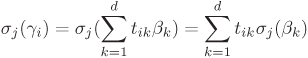
Proposition 2.46.

Δ(β1, . . . , βd) = (det(σj(βi)))2. Proof Consider the matrices D := (Tr(βiβj)) and E := (σj(βi)). By definition, we have Δ(β1, . . . , βd) = det D. We show that D = EEt, which implies that det D = (det E)2. The ij-th entry of EEt is where the last equality follows from Equation (2.15).

Let for some and let f(X) be the minimal polynomial of α over . We define the discriminant of f as

Δ(f) := Δ(1, α, α², ..., α^d–1).

We have to show that the quantity Δ(f) is well-defined, that is, independent of the choice of the root α of f(X). Let α = α₁, α₂, . . . .α_d be all the roots of f(X) and let the complex embedding σ_j of K map α to α_j. By Proposition 2.46, we have Δ(f) = (det E)², where . Computing the determinant of E gives 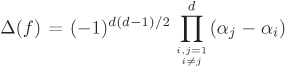, which implies that Δ(f) is independent of the permutations of the conjugates α₁, . . . , α_d of α. Notice that since α₁, . . . , α_d are all distinct, Δ(f) ≠ 0.

Let us deduce a useful formula for Δ(f). Write 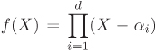and take formal derivative to get , that is, . Therefore, , that is,

Equation 2.16

For arbitrary , the discriminant Δ(β₁, . . . , β_d) discriminates between the cases that β₁, . . . , β_d form a -basis of K and that they do not.

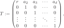
Lemma 2.12.

Let satisfy for i = 1, . . . , d and for . Then Δ(γ1, . . . , γd) = (det T)2Δ(β1, . . . , βd), where T = (tij). Proof Let E1 := (σj(βi)) and E2 := (σj(γi)). Now is the ij-th entry of the matrix T E1, that is, E2 = T E1. Hence Δ(γ1, . . . , γd) = (det E2)2 = (det T)2(det E1)2 = (det T)2Δ(β1, . . . , βd).

Corollary 2.19.

Let and be two -bases of K. Let and . Then , where T is the change-of-basis matrix from to .

Corollary 2.20.

form a -basis of K, if and only if Δ(β1, . . . , βd) ≠ 0. Proof Let , and . Since is a -basis of K, each βi can be written (uniquely) as with . By Lemma 2.12, , where . We have seen that . Therefore, is a -basis of K.

Finally comes the desired characterization of .

Theorem 2.55.

For a number field K of degree d, the ring is a free -module of rank d. Proof Let form a -basis of K. We know that for some the elements r1β1, . . . , rdβd are in and continue to constitute a -basis of K. So we may assume that the elements β1, . . . , βd are already in . Consider the set S of all -basis (β1, . . . , βd) of K consisting of elements from only. By Definition 2.104 and Corollary 2.20, for every . Choose such that is minimal in S. Claim: is linearly independent over . is a -basis of K, that is, linearly independent over and so trivially over too. Claim: generates as a -module. Assume not, that is, there exists such that α = a1β1 + · · · + adβd with some . Without loss of generality, we may assume that and write a1 = a + r with and 0 < r < 1. Define γ1 := α – aβ1 = rβ1 + a2β2 + · · · + adβd, γ2 := β2, . . . , γd := βd. Clearly, . Furthermore, if by Lemma 2.12, we have Δ(γ1, . . . , γd) = (det T)2Δ(β1, . . . , βd) = r2Δ(β1, . . . , βd). Since r ≠ 0, Δ(γ1, . . . , γd) ≠ 0, that is, (γ1, . . . , γd) is again a -basis of K (Corollary 2.20), that is, . Finally since r < 1, we have |Δ(γ1, . . . , γd)| < |Δ(β1, . . . , βd)|, a contradiction to the choice of (β1, . . . , βd). Thus every has to be a -linear combination of β1, . . . , βd. This completes the proof of the second claim and also of the theorem.

Definition 2.105.

Any -basis of is called an integral basis of K (or of ).

Corollary 2.21.

Every integral basis of K has the same discriminant (for a given K). Proof Let and be two integral bases of K. Let T be the -to- change-of-basis matrix. being an integral basis of K, all the entries of T are integers. Also from Corollary 2.19 we have and hence divides and has the same sign as . One can analogously show . Therefore, .

Definition 2.106.

Let be an integral basis of a number field K. The discriminant of K is defined to be the integer . By Corollary 2.21, ΔK is well-defined, that is, independent of the choice of the integral basis of K.

Recall that K, as a vector space over , always possesses a -basis of the form 1, α, . . . , α^d–1. , as a -module, is free of rank d, but every number field K need not possess an integral basis of the form 1, α, . . . , α^d–1. Whenever it does, is called monogenic and an integral basis 1, α, . . . , α^d–1 of K is called a power integral basis. Clearly, if K has a power integral basis 1, α, . . . , α^d–1, then . But the converse is not true, that is, for with , 1, α, . . . , α^d–1 need not be an integral basis of K, even when is monogenic.

Example 2.31.

Consider the quadratic number field for some square-free integer D ≠ 0, 1. We consider the two cases (See Exercise 2.136): Case 1: D ≡ 2, 3 (mod 4) Here , that is, is a power integral basis of K. The minimal polynomial of is X2 – D and the conjugates of are ±. Therefore, by Equation (2.16), we have Case 2: D ≡ 1 (mod 4) In this case, , that is, is a power integral basis of K. The minimal polynomial of is and the conjugates of are ±. Therefore, Equation (2.16) gives

2.13.3. Unique Factorization of Ideals

Ideals in a number ring possess very rich structures. We prove that number rings are Dedekind domains (Definition 2.99). A Dedekind domain (henceforth abbreviated as DD) need not be a UFD (or a PID). However, it is a ring in which ideals admit unique factorizations into products of prime ideals.

Let K be a number field of degree and its ring of integers. If is a homomorphism of rings and if is a prime ideal of B, then the contraction is a prime ideal of A. We say that lies above or over . If A ⊆ B and is the inclusion homomorphism, then . For a number field K, we consider the natural inclusion .

Lemma 2.13.

Let be a non-zero prime ideal of . Then lies above a unique non-zero prime ideal of . In particular, contains a (unique) rational prime. Proof Let . If , then both and 0 are prime ideals of that lie over the zero ideal of . Since , by Exercise 2.128(c), a contradiction.

Proposition 2.47.

is Noetherian. Proof Let constitute an integral basis of K, that is, , that is, the ring homomorphism mapping f(X1, . . . , Xd) ↦ f(α1, . . . , αd) is surjective. By Hilbert’s basis theorem (Theorem 2.8), the polynomial ring is Noetherian and so , being the quotient of a Noetherian ring (by the isomorphism theorem), is Noetherian too (Example 2.29).

Theorem 2.56.

The ring of integers of a number field K is a Dedekind domain. Proof We have proved that is Noetherian (Proposition 2.47) and integrally closed (Proposition 2.44). It then suffices to show that each non-zero prime ideal of is maximal. By Lemma 2.13, lies over a non-zero prime ideal of . But is maximal in . Exercise 2.128(b) now completes the proof.

Now we derive the unique factorization theorem for ideals in a DD. It is going to be a long story. We refer the reader to Definition 2.92 to recall how the product of two ideals is defined.

Lemma 2.14.

Let A be a ring, , ideals of A, and a prime ideal of A such that . Then for some . In particular, if A is a DD and are non-zero prime ideals, then for some . Proof The proof is obvious for r = 1. So assume that r > 1. If for all i = 1, . . . , r, then for each i we can choose and see that , a contradiction to that is prime. The last statement of the lemma follows from the fact that in a DD every non-zero prime ideal is maximal.

We now generalize the concept of ideals.

Definition 2.107.

Let A be an integral domain and K := Q(A). An A-submodule of K is called a fractional ideal of A, if for some .

Every ideal of A is evidently a fractional ideal of A and hence is often called an integral ideal of A. Conversely, every fractional ideal of A contained in A is an integral ideal of A. The principal fractional ideal Ax is the A-submodule of K generated by . If A is a Noetherian domain, we have the following equivalent characterization of fractional ideals.

Lemma 2.15.

Let A be a Noetherian integral domain, K := Q(A) and . Then is a fractional ideal of A, if and only if is a finitely generated A-submodule of K. Proof [if] Let , where xi = ai/bi, ai, , bi ≠ 0. Then . [only if] Let be such that . Now ba is an (integral) ideal of A (easy check) and is finitely generated, since A is Noetherian. Let , . Then , where .

We define the product of two fractional ideals , of an integral domain A as we did for integral ideals:

It is easy to check that is again a fractional ideal of A. Let denote the set of non-zero fractional ideals of A. The product of fractional ideals defines a commutative and associative binary operation on . The ideal A acts as a (multiplicative) identity in . A fractional ideal of A is called invertible, if for some fractional ideal of A. We deduce shortly that if A is a DD, then every non-zero fractional ideal of A is invertible and, therefore, is a group under multiplication of fractional ideals.

Lemma 2.16.

Let A be a Noetherian domain and an (integral) ideal of A. For some , there exist prime ideals of A each containing such that . Proof Let S be the set of ideals of A for which the lemma does not hold. Assume that . Since A is Noetherian, S contains a maximal element, say . Clearly, is a proper non-prime ideal of A, that is, for some a, we have . The ideals and strictly contain and, therefore, by the maximality of are not in S, that is, there exist prime ideals each containing (and hence ) such that and prime ideals each containing (and hence ) such that . Moreover, , since , so that , a contradiction. Thus S must be empty.

Note that the condition “each containing ” was necessary in Lemma 2.16 in order to rule out the trivial possibility that for some .

Lemma 2.17.

Let A be a DD, K := Q(A) and a non-zero prime ideal of A. Define the set . Then we have: is a fractional ideal of A. . . In particular, every non-zero prime ideal in a DD is invertible. Proof Clearly, is an A-submodule of K, and for , we have . Since , we have . In order to prove the strict inclusion, we take any and consider the ideal . By Lemma 2.16, there exist prime ideals each containing (and hence non-zero) such that . We choose r to be minimal, so that does not contain the product of any r – 1 of . Now and hence by Lemma 2.14 for some i, say, i = r. Choose any . Since , we have . On the other hand, and , so that , that is, . By the definition of , it follows that is contained in and hence an integral ideal of A. Since , it follows that . Since is a maximal ideal, we then have or . Assume that . We claim that this assumption implies that , a contradiction to Part (2). So we must have . For proving the claim, let and choose . Then we have and, therefore, and so on. For each , define the ideal . Then is an ascending chain of ideals in A. Since A is Noetherian, the chain must be stationary, that is, for some we have , that is, , that is, with . Since A is an integral domain and a ≠ 0, we see that b is integral over A. Since A is integrally closed, . Therefore, , as claimed.

Theorem 2.57.

Every non-zero ideal in a DD A can be represented as a product of prime ideals of A. Moreover, such a factorization of is unique up to permutations of the factors. Proof If , there is nothing to prove. So let be a proper ideal of A. We first show that if contains a product of non-zero prime ideals, then is a product of prime ideals. By Lemma 2.16, we have prime ideals , , of A each containing , such that . Let us choose r to be minimal and proceed by induction on r. If r = 1, is already prime. So take r > 1 and assume that if an ideal of A contains a product of r – 1 or less non-zero prime ideals of A, then is a product of prime ideals. Let be a maximal ideal containing . We then have and by Lemma 2.14 for some i, say, i = r. Now, consider the fractional ideal . Then and so is an integral ideal of A. Furthermore , that is, contains a product of r – 1 non-zero prime ideals. By the induction hypothesis, is a product of prime ideals, that is, . But then is also a product of prime ideals. In order to prove the uniqueness of this product, let with prime ideals and . Now and by Lemma 2.14 for some , say, j = 1. Then . Proceeding in this way shows the desired uniqueness.

In the factorization of a non-zero ideal of a DD, we do not rule out the possibility of repeated occurrences of factors. Taking this into account shows that every non-zero ideal in a DD A admits a unique factorization

with distinct non-zero prime ideals and with exponents . Here uniqueness is up to permutations of the indexes 1, . . . , r. This factorization can be extended to fractional ideals, but this time we have to allow non-positive exponents. First note that for integers e₁, . . . , e_r and non-zero prime ideals of A the product is well-defined and is a fractional ideal of . The converse is proved in the following corollary.

Corollary 2.22.

Every non-zero fractional ideal of a DD A admits a unique factorization of the form with non-zero prime ideals of A and with exponents . Moreover for such a fractional ideal we have . Proof By definition, there exists such that . But then is an integral ideal of A. We write and with fi, . Since each non-zero prime ideal is invertible (Lemma 2.17(3)), it follows that . This proves the existence of a factorization of . The proof for the uniqueness is left to the reader as an easy exercise. The last assertion follows from a repeated use of Lemma 2.17(3).

The fractional ideal in Corollary 2.22 is denoted by . We have . One can easily verify that defined as above is equal to the set

In fact, one can use the last equality as the definition for .

To sum up, every non-zero fractional ideal of a DD A is invertible and the set of all non-zero fractional ideals of A is a group. The unit ideal A acts as the identity in .

As in every group, we have the cancellation law(s) in .

Corollary 2.23.

Let A be a DD and , , fractional ideals of A. If and , then .

In view of unique factorization of ideals in A, we can speak of the divisibility of integral ideals in A. Let and be two integral ideals of A. We say that divides and write , if for some integral ideal of A. We now show that the condition is equivalent to the condition . Thus for ideals in a DD the term divides is synonymous with contains.

Corollary 2.24.

Let and be integral ideals of a DD A. Then if and only if . Proof [if] If , we have , that is, is an integral ideal of A. Also . [only if] If for some integral ideal , we have .

Corollary 2.25.

Let and with ei, be the prime decompositions of two non-zero integral ideals of a DD A. Then if and only if ei ≤ fi for all i = 1, . . . , r. Proof [if] We have , where is an integral ideal of A. [only if] Let for some integral ideal of A. Clearly, and we can write the prime decomposition with li ≥ 0. We have . By unique factorization, we have f1 = e1 + l1, . . . , fr = er + lr and lr+1 = · · · = lr+s = 0.

As we pass from to , the notion of unique factorization passes from the element level to the ideal level. If a DD is already a PID, these two concepts are equivalent. (Non-zero prime ideals in a PID are generated by prime elements.) Though every UFD need not be a PID, we have the following result for a DD.

Proposition 2.48.

A Dedekind domain A is a UFD, if and only if A is a PID. Proof [if] Every PID is a UFD (Theorem 2.11). [only if] Let A be a UFD. In order to show that A is a PID, it suffices (in view of Theorem 2.57) to show that every non-zero prime ideal of A is a principal ideal. Choose any non-zero . Then . Now a is a non-unit in A (since otherwise we would have ) and A is assumed to be a UFD. Thus we can write a = uq1 · · · qr for , and for prime elements qi in A. Clearly, each 〈qi〉 is a non-zero prime ideal of A and 〈a〉 = 〈q1〉 · · · 〈qr〉. Therefore, and hence by Lemma 2.14 for some .

In the rest of this section, we abbreviate as , if K is implicit in the context.

2.13.4. Norms of Ideals

We have seen that the ring is a free -module of rank d. The same result holds for every non-zero ideal of . Let β₁, . . . , β_d constitute an integral basis of K.

One can choose rational integers a_ij with each a_ii positive such that

Equation 2.17

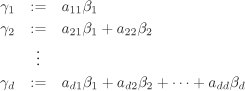
constitute a -basis of . Moreover, the discriminant Δ(γ₁, . . . , γ_d) is independent of the choice of an integral basis γ₁, . . . , γ_d of and is called the discriminant of , denoted . It follows that can be generated as an ideal (that is, as an -module) by at most d elements. We omit the proof of the following tighter result.

Proposition 2.49.

Every (integral) ideal in a DD A is generated by (at most) two elements. More precisely, for a proper non-zero ideal of A and for any there exists with .

Definition 2.108.

The norm of a non-zero ideal of is defined as the cardinality of the quotient ring . It is customary to define the norm of the zero ideal as zero.

Using the integers a_ij of Equations (2.17), we can write

Equation 2.18

Corollary 2.26.

For every non-zero ideal of , the quotient ring is a finite ring. In particular, if is a non-zero prime (hence maximal) ideal of , then is a finite field.

It is tempting to define the norm of an element to be the norm of the principal ideal . It turns out that this new definition is (almost) the same as the old definition of N(α). More precisely:

Proposition 2.50.

For any element , we have N(〈α〉) = |N(α)|. Proof The result is obvious for α = 0. So assume that α ≠ 0 and call . Let β1, . . . , βd be an integral basis of . It is an easy check that αβ1, . . . , αβd is an integral basis of . Let σ1, . . . , σd be the complex embeddings of K. Then is the square of the determinant of the matrix It follows that . Equation (2.18) now completes the proof.

Corollary 2.27.

For any , we have .

Like the norm of elements, the norm of ideals is also multiplicative. We omit the (not-so-difficult) proof here.

Proposition 2.51.

Let and be ideals in . Then, .

The following immediate corollary often comes handy.

Corollary 2.28.

Let and be non-zero ideals of . If is the factorization of , then . In particular, if , then (in ).

2.13.5. Rational Primes in Number Rings

The behaviour of rational primes in number rings is an interesting topic of study in algebraic number theory. Let K be a number field of degree d and . Consider a rational prime p and denote by 〈p〉 the ideal generated by p in . We use the symbol to denote the (prime) ideal of generated by p. Further let

Equation 2.19

be the prime factorization of 〈p〉 with , with pairwise distinct non-zero prime ideals of and with . For each i, we have , that is, , that is, (Lemma 2.13), that is, lies over . Conversely if is an ideal of lying over , then , that is, , that is, , that is, for some i. Thus, are precisely all the prime ideals of that lie over .

By Corollary 2.27, N(〈p〉) = p^d. By Corollary 2.28, each divides p^d and is again a power p^di of p.

Definition 2.109.

We define the ramification index of over p (or ) as . This is the largest such that divides (that is, contains) 〈p〉. The integer di (where is called the inertial degree of over p.

By the multiplicative property of norms, we have

Definition 2.110.

If r = d, so that each ei = di = 1, we say that the prime p (or )splits completely in . On the other extreme, if r = 1, e1 = 1, d1 = d, then 〈p〉 is prime in and we say that p is inert in . Finally, if ei > 1 for some i, we say that the prime p ramifies in . If r = 1 and e1 = d (so that d1 = 1), then the prime p is said to be totally ramified in .

The following important result is due to Dedekind. Its proof is long and complicated and is omitted here.

Theorem 2.58.

A rational prime p ramifies in , if and only if p divides the discriminant ΔK. In particular, there are only finitely many rational primes that ramify in .

Though this is not the case in general, let us assume that the ring is monogenic (that is, for some ) and try to compute the explicit factorization (Equality (2.19)) of 〈p〉 in . In this case, and let be the minimal polynomial of α. We then have .

Let us agree to write the canonical image of any polynomial in as . We write the factorization of as

with and with pairwise distinct irreducible polynomials . If , then . For each i = 1, . . . , r choose whose reduction modulo p is . Define the ideals

of . Since , we have

and

Therefore, are non-zero prime ideals of with . Thus . On the other hand, , since f(α) = 0 and . Thus we must have , that is, we have obtained the desired factorization of 〈p〉.

Let us now concentrate on an example of this explicit factorization.

Example 2.32.

Let D ≠ 0, 1 be a square-free integer congruent to 2 or 3 modulo 4. If , then is monogenic. We take an odd rational prime p and compute the factorization of 〈p〉 in . We have to factorize modulo p the minimal polynomial f(X) := X2 – D. We consider three cases separately based on the value of the Legendre symbol . Case 1: In this case, p|D, that is, . Then , where . Thus p (totally) ramifies in . Case 2: Since p is assumed to be an odd prime, the two square roots of D modulo p are distinct. Let δ be an integer with δ2 ≡ D (mod p). Then . In this case, , where and . Thus p splits (completely) in . Case 3: The polynomial is irreducible in and hence remains prime in , that is, p is inert in . Thus the quadratic residuosity of D modulo p dictates the behaviour of p in . Let us finally look at the fate of the even prime 2 in . If D is even, then and if D is odd, then . In each case, 2 ramifies in . Recall from Example 2.31 that ΔK = 4D. Thus we have a confirmation of the fact that a rational prime p ramifies in if and only if p|ΔK.

One can similarly study the behaviour of rational primes in

,

where D ≡ 1 (mod 4) is a square-free integer ≠ 0, 1.

2.13.6. Units in a Number Ring

There are just two units in , namely ±1. In a general number ring, there may be many more units. For example, all the units in the ring of Gaussian integers are ±1, ±i. There may even be an infinite number of units in a number ring. It can be shown that , , are all the units of . (Note that for all n ≠ 0 the absolute values of are different from 1.) is a PID. So we can think of factorizations in as element-wise factorizations. To start with, we fix a set of pairwise non-associate prime elements of . Every non-zero element of admits a factorization for prime “representatives” p_i and for a unit u of the form . Thus, in order to complete the picture of factorization, we need machinery to handle the units in a number ring.

Let K be a number field of degree d and signature (r₁, r₂). We have d = r₁ + 2r₂. The set of units in is denoted by . We know that is an (Abelian) group under (complex) multiplication. Our basic aim now is to reveal the structure of the group .

Every Abelian group is a -module and, if finitely generated and not free, contains torsion elements, that is, (non-identity) elements of finite order > 1.^[19] always contains the element –1 of order 2. The torsion subgroup of is denoted by . We have , where is a torsion-free group. It turns out that ℜ is a finite group (and hence cyclic) and that is finitely generated and hence free, that is, for some . From Dirichlet’s unit theorem (which we do not prove), it follows that ρ = r₁ + r₂ – 1. Thus, has a -basis consisting of ρ elements, say ξ₁, . . . , ξ_ρ, and every unit of can be uniquely expressed as , where ω is a root of unity and . A set of generators of is called a set of fundamental units.

^[19] Every finitely generated torsion-free module over a PID is free.

Example 2.33.

Let D ≠ 0, 1 be a square-free integer, and . If D < 0, the signature of K is (0, 1) and the value of ρ for is 0 + 1 – 1 = 0, that is, , that is, is finite in this case. Now, suppose D > 0. K is a real field in this case, so that . Also the signature of K is (2, 0), that is, ρ = 2 + 0 – 1 = 1. This means that contains an infinite number of units. Let ξ be a fundamental unit of . Then, every unit of is of the form ±ξn, .

Exercise Set 2.13

2.126	If A ⊆ B and B ⊆ C are integral extensions of rings, show that A ⊆ C is also an integral extension. Let A ⊆ B be an extension of rings. Show that the integral closure of A in B is integrally closed in B. Let A ⊆ B be an integral extension of rings, an ideal of B and . (Note that is an ideal of A. If is prime in B, then is prime in A. See Proposition 2.10.) Show that is integral over .
2.127	Let A ⊆ B be an extension of integral domains, a finitely generated non-zero ideal of A and . If , show that γ is integral over A. [H]
2.128	Let A ⊆ B be an integral extension of integral domains. Show that A is a field if and only if B is a field. Let A ⊆ B be an integral extension of rings, a prime ideal of B and . Show that is maximal if and only if is maximal. [H] Let A, B, and be as in (b). Further let be another prime ideal of B with . Show that if , then . [H]
2.129	Let A be a ring and S a multiplicatively closed subset of A. Show that: If , then S–1A is the zero ring. If S′ := S {1} is non-empty and closed under multiplication, then S′–1A ≅ S–1A. If A is Noetherian, then S–1A is also Noetherian.
2.130	Let A ⊆ B be a ring extension and C the integral closure of A in B. Show that for any multiplicative subset S of A (and hence of B and C) the integral closure of S–1A in S–1B is S–1C. In particular, if A is integrally closed in B, then so is S–1A in S–1B.
2.131	Recall that an integrally closed integral domain is called a normal domain (ND). Show that every UFD is a normal domain. Let D be a square-free integer ≠ 0, 1. Show that , is normal if and only if D ≡ 2, 3 (mod 4). (Remark: The reader should note the following important implications: That is, a Euclidean domain is a PID, a PID is a UFD and a UFD is a normal domain. Neither of the reverse implications is true. For example, the ring of integers of is known to be a PID but not a Euclidean domain. The ring K[X1, . . . , Xn], n ≥ 2, of multivariate polynomials over a field K is a UFD, but not a PID, since the ideal 〈X1, . . . , Xn〉 is not principal. Finally, is a normal domain (by Exercise 2.136 below), but not a UFD, since are two different factorizations of 6 into irreducible elements.)
2.132	A (non-zero) ring A with a unique maximal ideal m is called a local ring. In that case, the field A/m is called the residue field of A. Let A be ring and a prime ideal of A. Show that the localization is a local ring with the unique maximal ideal generated by elements , and the residue field is canonically isomorphic to the quotient field of the integral domain under the map .
2.133	A ring A is called a discrete valuation ring (DVR) or a discrete valuation domain (DVD), if A is a local principal ideal domain. Let A be a DVR with maximal ideal m = 〈p〉. Prove the following assertions: A is a UFD. The only primes in A are the associates of p. [H] Every non-zero element of A can be written as upα, where u is a unit of A and . Every non-zero ideal of A is of the form 〈pα〉 for some . A has only one non-zero prime ideal (namely, m). (Remark: The prime p of A is called a uniformizing parameter or a uniformizer for A and is unique up to multiplication by units. The map taking upα ↦ α is called a discrete valuation of A and can be naturally extended to a group homomorphism by defining ν(a/b) := ν(a)–ν(b), where a, , b ≠ 0 and K = Q(A) is the quotient field of A. It is often convenient to define ν(0) := +∞. It follows that and .)
2.134	Let A be a local Noetherian integral domain which is not a field. Assume further that the maximal ideal m ≠ 0 of A is the only non-zero prime ideal of A. Show that A is a DVR (that is, a PID) if and only if A is integrally closed. Let A be a Noetherian integral domain which is not a field. Prove that A is a Dedekind domain if and only if is a DVR for every non-zero prime ideal of A.
2.135	Show that the only units of are ±1 and ±i. Show that the primes of are associates to the following: a prime integer ≡ 3 (mod 4), a + ib, a, , with a2 + b2 equal to 2 or a prime integer ≡ 1 (mod 4).
2.136	Show that every quadratic number field K can be represented as for a square-free integer D ≠ 0, 1. Let for some square-free integer D ≠ 0, 1. Show that: (In particular, the ring of integers of is the ring of Gaussian integers.)
2.137	Let A be a Dedekind domain. Let q1 and q2 be two distinct non-zero prime ideals of A. Show that for any e1, we have . [H] Let be the prime factorization of a non-zero ideal of A with pairwise distinct primes qi and . Show that . [H]
2.138	Let A be a Dedekind domain and a non-zero (integral) ideal of A. Show that: There exists a non-zero (integral) ideal of A such that is a principal ideal. [H] The number of ideals of A containing is finite. Every ideal of is principal.
2.139	Let and , ei, , be the prime decompositions of two non-zero ideals , of a DD A. Define the gcd and lcm of and as Show that and lcm. Conclude that . (Note that if A is a general ring, we only have .)
2.140	Let K be a number field and . Let be an ideal of . Show that . In particular, every non-zero ideal of contains a non-zero integer. [H] Let be a non-zero prime ideal of . Prove that for some , where p is the unique rational prime contained in (Lemma 2.13).
2.141	Let K be a number field, , , and . Show that: , if and only if N(α) = ±1. , if and only if f(0) = ±1, where is the minimal polynomial of α over . , if and only if |σ(α)| = 1 for every complex embedding σ of K.
2.142	Let K be a number field. We say that K is norm-Euclidean, if for every α, , β ≠ 0, there exist q, such that α = qβ + r and | N(r)| < | N(β)|. Conclude that if K is norm-Euclidean, then is a Euclidean domain with the Euclidean degree function ν(α) := | N(α)|. (The converse of this is not true. For example, it is known that is not norm-Euclidean, but is a Euclidean domain.) Prove the following equivalent characterization of a norm-Euclidean number field: K is norm-Euclidean if and only if for every there exists such that | N(α – β)| < 1. Show that the following number fields are norm-Euclidean: , , , and . Show that is not norm-Euclidean. [H]
2.143	In this exercise, one derives that the only (rational) integer solutions of Bachet’s equation Equation 2.20 are x = 3, y = ±5. Show that Equation (2.20) has no solutions with x or y even. [H] Let (x, y) be a solution of Equation (2.20) with both x and y odd. Then x3 admits a factorization in as . Let . Show that and that is a UFD. Also the only units of are ±1. Show that gcd. [H] Because of unique factorization one can write for c, . Expand the cube and equate the real and imaginary parts to conclude that we must have y = ±5, so that x = 3.