*2.11. Elliptic Curves

The mathematics of elliptic curves is vast and complicated. A reasonably complete understanding of elliptic curves would require a book of comparable size as this. So we plan to be rather informal while talking about elliptic curves and about their generalizations called hyperelliptic curves. Interested readers can go through the books suggested at the end of this chapter to learn more about these curves. In this section, K stands for a field (finite or infinite) and the algebraic closure of K.

2.11.1. The Weierstrass Equation

An elliptic curve E over K is a plane curve defined by the polynomial equation

Equation 2.6

or by the corresponding homogeneous equation

E : Y²Z + a₁XYZ + a₃YZ² = X³ + a₂X²Z + a₄XZ² + a₆Z³.

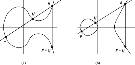
These equations are called the Weierstrass equations for E. In order that E qualifies as an elliptic curve, we additionally require that it is smooth at all -rational points (Definition 2.66).^[12] Two elliptic curves defined over the field are shown in Figure 2.1.

^[12] Ellipses are not elliptic curves.

E contains a single point at infinity, namely (Exercise 2.97(e)). The set of K-rational points on E in the projective plane is denoted by E(K) and is the central object of study in the theory of elliptic curves. We shortly endow E(K) with a group structure and this group is used extensively in cryptography.

Let us first see how we can simplify the equation for E. The simplification depends on the characteristic of K. Because fields of characteristic 3 are only rarely used in cryptography, we will not deal with such fields. Simplification of the Weierstrass equation is effected by suitable changes of coordinates. A special kind of transformation is allowed in order to preserve the geometric and algebraic properties of an elliptic curve.

Theorem 2.44.

Two elliptic curves E1 : Y2 + a1XY + a3Y = X3 + a2X2 + a4X + a6 E2 : Y2 + b1XY + b3Y = X3 + b2X2 + b4X + b6 defined over K are isomorphic (Definition 2.72) if and only if there exist and r, s, such that the substitution of u2X + r for X and u3Y + u2sX + t for Y transforms the equation of E1 to the equation of E2. For this transformation, the coefficients bi are related to the coefficients ai as follows: Equation 2.7

The theorem is not proved here. Formulas (2.7) can be checked by tedious calculations. A change of variables as in Theorem 2.44 is referred to as an admissible change of variables. We denote this by

(X, Y) ← (u²X + r, u³Y + u²sX + t).

The inverse transformation is also admissible and is given by

Isomorphism is an equivalence relation on the set of all elliptic curves over K.

Consider the elliptic curve E over K given by Equation (2.6). If char K ≠ 2, the admissible change transforms E to the form

E₁ : Y² = X³ + b₂X² + b₄X + b₆.

If, in addition, char K ≠ 3, the admissible change transforms E₁ to E₂ : Y² = X³ + aX + b. We henceforth assume that an elliptic curve over a field of characteristic ≠ 2, 3 is defined by

Equation 2.8

(instead of by the original Weierstrass Equation (2.6)).

If char K = 2, the Weierstrass equation cannot be simplified as in Equation (2.8). In this case, we consider two cases separately, namely a₁ ≠ 0 or otherwise. In the former case, the admissible change allows us to write Equation (2.6) in the simplified form

Equation 2.9

On the other hand, if a₁ = 0, then the admissible change (X, Y) ← (X + a₂, Y) shows that E can be written in the form

Equation 2.10

A curve defined by Equation (2.9) is called non-supersingular, whereas one defined by Equation (2.10) is called supersingular.

Now we associate two quantities with an elliptic curve. The importance of these quantities follows from the subsequent theorem. We start with the generic Weierstrass equation and later specialize to the simplified formulas.

Definition 2.76.

For the curve given by Equation (2.6), we define the following quantities: Equation 2.11 Δ(E) is called the discriminant of the curve E, and j(E) the j-invariant of E.

For the special cases given by the simplified equations above, these quantities have more compact formulas as given in Table 2.5.

Theorem 2.45.

For the curve E defined by Equation (2.6), the following properties hold: An admissible change of variables does not alter Δ(E) and j(E). Table 2.5. Discriminant and j-invariant for elliptic curves Special case Δ(E) j(E) char K ≠ 2, 3 (Equation 2.8) –16(4a3 + 27b2) 1728(4a)3/Δ(E) char K = 2, non-supersingular (Equation 2.9) b 1/b char K = 2, supersingular (Equation 2.10) a4 0 E is an elliptic curve, that is, E is smooth, if and only if Δ(E) ≠ 0. In particular, the j-invariant is defined for all elliptic curves. Let E1 and E2 be two elliptic curves defined over the field K. If E1 and E2 are isomorphic over K, then j(E1) = j(E2). Conversely, if j(E1) = j(E2), then E1 and E2 are isomorphic over . Proof Tedious calculations using Formulas (2.7) establish this claim. The polynomial f(X, Y, Z) = Y2Z + a1XYZ + a3YZ2 – X3 – a2X2Z – a4XZ2 – a6Z3 defines the curve E. Since , E is smooth at . Suppose that E is not smooth at the finite point . The admissible change (X, Y) ← (X + x0, Y + y0) does not alter the value of Δ(E) by (1). So we can assume, without loss of generality, that (x0, y0) = (0, 0). But then we have f(0, 0) = –a6 = 0, ∂f/∂x(0, 0) = –a4 = 0 and ∂f/∂y(0, 0) = a3 = 0. Now it is easy to check from Equation (2.11) that Δ(E) = 0. Conversely, let Δ(E) = 0. For simplicity, we assume that char K ≠ 2, 3 and E is given by Equation (2.8). By Exercise 2.62, , that is, the polynomial X3 + aX + b has multiple roots, say, . But then E is not smooth at . By Part (1) and Theorem 2.44, two isomorphic elliptic curves have the same j-invariant. For proving the converse, we once again assume that char K ≠ 2, 3 and E1 : Y2 = X3 + a1X + b1 and E2 : Y2 = X3 + a2X + b2 have the same j-invariant. Then we have . Now we provide an admissible change of variable of the form (X, Y) ← (u2X, u3Y), , that transforms E1 to E2. Since Δ(E1) ≠ 0 and Δ(E2) ≠ 0, we take u = (b1/b2)1/6 if a1 = 0, u = (a1/a2)1/4 if b1 = 0, and u = (a1/a2)1/4 = (b1/b2)1/6 if a1b1 ≠ 0. Note that since is algebraically closed, u is defined in all the above cases.

2.11.2. The Elliptic Curve Group

Consider an elliptic curve E over a field K. We now define an operation (which is conventionally denoted by +) on the set E(K) of K-rational points on E in the projective plane . This operation provides a group structure on E(K). It is important to point out that this group is not the same as the group Div_K(E) of divisors on E(K) (Definition 2.74), since the sum of points we are going to define is not formal. However, there is a connection between these two groups (See Exercise 2.125).

Definition 2.77.

Let E be the elliptic curve defined by Equation (2.6) and the point at infinity on E. A binary operation + on E(K) is defined as follows: For any , we define , that is, serves as the additive identity. The opposite (additive inverse) of a point is now defined: if , then –P = P, and if , then –P = (h, –k – a1h – a3). For P, , the sum P + Q is defined by the chord and tangent rule which goes as follows. If Q = –P, then . If Q ≠ –P, we consider the line passing through P and Q (we take the tangent line if P = Q). Since the degree of the defining equation for E is three, this line meets the curve at exactly one other point R. We define P + Q = –R. Figure 2.1 illustrates this case for curves over .

Theorem 2.46.

The set E(K) under the operation + is an Abelian group.

No simple proof of this theorem is known. Indeed the only group axiom that is difficult to check is associativity, that is, to check that (P + Q) + R = P + (Q + R) for all P, Q, . An elementary strategy would be to write explicit formulas for (P + Q) + R and P + (Q + R) (using the formulas for P + Q given below) and show that they are equal, but this process involves a lot of awful calculations and consideration of many cases.

There are other proofs that are more elegant, but not as elementary. One possibility is to use the theory of divisors and is outlined now. It turns out that the Jacobian has a bijective correspondence with the set E(K) via the map which takes to (more correctly to the equivalence class of the divisor in ). Furthermore, , where the addition on the left is the addition on E(K) as defined above and the addition on the right is that in the Jacobian . By definition, is naturally an additive Abelian group. It immediately follows that E(K) is an additive Abelian group too. (See Exercise 2.125.)

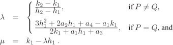
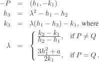
We now give the formulas for the coordinates of the points –P and P + Q on E(K). The derivation of these formulas for the general case is left to the reader (Exercise 2.102). We concentrate on the important special cases. We assume that P = (h₁, k₁) and Q = (h₂, k₂) are finite points on E(K) with Q ≠ –P so that .

If char K ≠ 2, 3 and E is defined by Equation 2.8, we have:

Next, we consider char K = 2 and non-supersingular curves (Equation 2.9). The formulas in this case are:

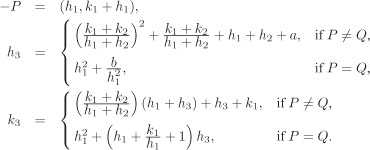
Finally, for supersingular curves (Equation 2.10) with char K = 2, we have:

We denote by mP the sum P + · · · + P (m times) for a point and for . We also define and (–m)P := –(mP) (for ).

Example 2.22.

Consider the elliptic curve E1 : Y2 = X3 + X + 3 over . We have Δ(E1) ≡ –16(4 × 13 + 27 × 32) ≡ 3 (mod 7). Also j(E1) ≡ 1728 × 43 × 3–1 ≡ 2 (mod 7), that is, j(E1) = 2. It is easy to check that contains the six points , P1 = (4, 1), P2 = (4, 6), P3 = (5, 0), P4 = (6, 1) and P5 = (6, 6). The multiples of these points are summarized in Table 2.6. It follows that the group is cyclic with P1 as a generator. Table 2.6. Multiples of points on the elliptic curve Y2 = X3 + X + 3 over P 2P 3P 4P 5P 6P ord P           1 P1 = (4, 1) (6, 6) (5, 0) (6, 1) (4, 6) 6 P2 = (4, 6) (6, 1) (5, 0) (6, 6) (4, 1) 6 P3 = (5, 0)         2 P4 = (6, 1) (6, 6)       3 P5 = (6, 6) (6, 1)       3 Now, consider the non-supersingular elliptic curve E2 : Y2 + XY = X3 + X2 + ξ defined over , where ξ := T + 〈T3 + T + 1〉. We have Δ(E2) = ξ and j(E2) = ξ–1 = ξ2 + 1. The finite points on E2 are: P1 = (0, ξ2 + ξ), P2 = (1, ξ2), P3 = (1, ξ2 + 1), P4 = (ξ, ξ2), P5 = (ξ, ξ2 + ξ), P6 = (ξ + 1, ξ2 + 1), P7 = (ξ + 1, ξ2 + ξ), P8 = (ξ2 + ξ, 1), P9 = (ξ2 + ξ, ξ2 + ξ + 1). So contains 10 points (including ). The multiples of the points are listed in Table 2.7, which implies that is again cyclic.[13] The φ(10) = 4 generators of this group are P4, P5, P8 and P9. [13] Both 6 and 10 are square-free integers, and so the groups and must be cyclic (Exercise 2.115(a)). Table 2.7. Multiples of points on the elliptic curve Y2 + XY = X3 + X2 + ξ over . P 2P 3P 4P 5P 6P 7P 8P 9P 10P ord P P0                   1 P1                 2 P2 P7 P6 P3           5 P3 P6 P7 P2           5 P4 P3 P9 P6 P1 P7 P8 P2 P5 10 P5 P2 P8 P7 P1 P6 P9 P3 P4 10 P6 P2 P3 P7           5 P7 P3 P2 P6           5 P8 P6 P4 P2 P1 P3 P5 P7 P9 10 P9 P7 P5 P3 P1 P2 P4 P6 P8 10 Let us continue to represent as in (2). The supersingular curve E3 : Y2 + Y = X3 + ξX + ξ2 has Δ(E3) = 1, j(E3) = 0. is a cyclic group with 9 points as Table 2.8 illustrates.

Table 2.8. Multiples of points on the elliptic curve Y² + Y = X³ + ξX + ξ² over

P	2P	3P	4P	5P	6P	7P	8P	9P	ord P
P0 =									1
P1 = (0, ξ2 + ξ)	P5	P4	P7	P8	P3	P6	P2		9
P2 = (0, ξ2 + ξ + 1)	P6	P3	P8	P7	P4	P5	P1		9
P3 = (ξ + 1, ξ)	P4								3
P4 = (ξ + 1, ξ + 1)	P3								3
P5 = (ξ2, ξ2)	P7	P3	P2	P1	P4	P8	P6		9
P6 = (ξ2, ξ2 + 1)	P8	P4	P1	P2	P3	P7	P5		9
P7 = (ξ2 + ξ, ξ2 + ξ)	P2	P4	P6	P5	P3	P1	P8		9
P8 = (ξ2 + ξ, ξ2 + ξ +1)	P1	P3	P5	P6	P4	P2	P7		9

Definition 2.78.

Let . The set of points such that is evidently a subgroup of E(K) and is denoted by EK[m] or by E[m], if K is understood from the context. The elements of EK[m], called the m-torsion points of E, are those points of E(K), the (additive) orders of which are finite and divide m.

Multiples mP of a point can be expressed using nice formulas.

Definition 2.79.

For an elliptic curve defined over K by the equation E : f(X, Y) = 0 and for , there exist polynomials θm, ωm, , such that for any point with we have mP = (θm(h, k)/ψm(h, k)2, ωm(h, k)/ψm(h, k)3). The polynomial ψm is called the m-th division polynomial of E.

Using the addition formula one can verify the following recursive description for ψ_m and the expressions for θ_m and ω_m in terms of ψ_m.

Lemma 2.8.

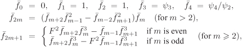
For an elliptic curve E defined by the general Weierstrass Equation (2.6) over a field K, the division polynomials ψm, , are recursively described as: where di are as in Definition 2.76. The polynomials θm satisfy for all , and for char K ≠ 2, one has

It follows by induction on m that these formulas really give polynomial expressions for ψ_m, θ_m and ω_m for all . For even m, the polynomial ψ_m is divisible by ψ₂. Furthermore, for the polynomials defined as

can be expressed as polynomials in x only. These univariate polynomials are easier to handle than the bivariate ones ψ_m and, by an abuse of notation, are also called division polynomials. The degrees of satisfy the inequality:

Points of E[m] can be characterized in terms of the division polynomials:

Theorem 2.47.

Ler and . Then if and only if ψm(h, k) = 0. Furthermore, if m > 2 and , then if and only if .

We finally define polynomials as follows. If char K ≠ 2, then for all . On the other hand, for char K = 2 and for non-supersingular curves over K we already have (Exercise 2.107), and it is customary to define f_m(x) := ψ_m(x, y) for all . By further abuse of notations, we also call f_m the m-th division polynomial of E.

2.11.3. Elliptic Curves over Finite Fields

In this section, we take , a finite field of cardinality q and characteristic p. We do not deal with the case p = 3. Let E be an elliptic curve defined over . If p > 3, we assume that E is defined by Equation (2.8), whereas for p = 2, we assume that E is defined by Equation (2.10) or Equation (2.9) depending on whether E is supersingular or not.

Since is a subset of , the cardinality is finite. The next theorem shows that is quite close to q.

Theorem 2.48. Hasse’s theorem

, where . (The integer t is called the trace of Frobenius at q.)

The implication of this theorem is that the possible cardinalities of lie in a rather narrow interval . If q = p is a prime, then for every n, , there is at least one curve E with . Moreover, the values of are distributed almost uniformly in the interval . However, if q is not a prime, these nice results do not continue to hold.

Definition 2.80.

If t = 1 (that is, if ), the curve E is called anomalous. If p|t, the curve E is called supersingular and if pt, then E is called non-supersingular.

Anomalous and supersingular curves are cryptographically weak, because certain algorithms are known with running time better than exponential to solve the so-called elliptic curve discrete logarithm problem over these curves. Determination of the order gives t from which one can easily check whether E is anomalous or supersingular. If p = 2, we have an easier check for supersingularity.

Proposition 2.35.

An elliptic curve E over a finite field of characteristic 2 is supersingular if and only if j(E) = 0 or, equivalently, if and only if a1 = 0 in Equation (2.6).

For arbitrary characteristic p, we have the following characterization.

Proposition 2.36.

An elliptic curve E over is supersingular if and only if t2 = 0, q, 2q, 3q or 4q. In particular, if char , 3, then E is supersingular if and only if t = 0.

By Theorem 2.38, the group is always cyclic. However, the group is not always cyclic, but is of a special kind. We need a few definitions to explain the structure of . The notion of internal direct product for multiplicative groups (Exercise 2.19) can be readily applied to additive groups as follows.

Definition 2.81.

Let G be an additive group and let H1, . . . , Hr be subgroups of G. If every element of G can be written uniquely as h1 + · · · + hr with , i = 1, . . . , r, we say that G is the (internal) direct sum of the subgroups H1, . . . , Hr and denote this as G = H1 ⊕ · · · ⊕ Hr.

Theorem 2.49. Structure theorem for finite Abelian groups

Let G be a finite additive Abelian group of cardinality #G = n. Then there exist and integers ni ≥ 2 for 1 ≤ i ≤ r, such that G is the direct sum of (subgroups isomorphic to the) cyclic groups , that is, , where ni+1|ni for all i = 1, . . . , r – 1. Furthermore, such a decomposition is unique in the sense that if with integers mi ≥ 2 and mi+1|mi for i = 1, . . . , s – 1, then r = s and ni = mi for all i = 1, . . . , r. In this case, we say that G has rank r and is of type (n1, . . . , nr). By Lagrange’s theorem, each ni|n. Moreover, n = n1n2 · · · nr. G is cyclic if and only if the rank of G is 1.

Theorem 2.50. Structure theorem for

The elliptic curve group is of rank 1 or 2. If the rank is 1, then is cyclic, otherwise , where n1, n2 ≥ 2 and n2|n1. In the second case, we have n2|(q – 1).

Once we know the order of the group , it is easy to compute the order of as the following theorem suggests.

Theorem 2.51.

Let α, satisfy 1 – tX + qX2 = (1 – αX)(1 – βX). Then for any the order .

Exercise Set 2.11

2.100	Show that the following curves over K are not smooth (and hence not elliptic curves): Y2 = X3, K arbitrary. Y2 = X3 + X2, K arbitrary. Y2 = X3 + aX + b, if char K = 2.
2.101	Show that for an elliptic curve E over K and a finite point , the only points in E(K) (or ) having X-coordinate equal to h are P and –P. Let char K ≠ 2, 3 and let E be defined by Equation (2.8). If α1, α2, are the roots (distinct by Theorem 2.45) of X3 + aX + b, then (α1, 0), (α2, 0) and (α3, 0) are the only points on with Y-coordinate equal to 0. Show that these are the only points of order 2 in .
2.102	Let P = (h1, k1) and Q = (h2, k2) be two points (different from ) in E(K) defined by the Weierstrass Equation (2.6). Assume that Q ≠ –P. Determine R = (h3, k3) = P + Q as follows: Show that the line passing through P and Q (the tangent, if P = Q) has the equation Y = λX + μ, where Substituting λX + μ for Y in Equation (2.6) gives a cubic equation in X of which h1 and h2 are two roots. Show that the third root (the X-coordinate of R) is h3 = λ2 + a1λ – a2 – h1 – h2. Hence deduce that the Y-coordinate of R is k3 = –(λ + a1)h3 – μ – a3.
2.103	Let . Show that there exists an elliptic curve E over K such that . [H]
2.104	Assume that char K ≠ 2, 3 and consider the elliptic curve E given by Equation (2.8). Let K[E] be the affine coordinate ring and K(E) the field of rational functions on E. Show that every element in K[E] can be uniquely represented as u(x) + yv(x) for polynomials u(x), . The conjugate of is defined as . The norm of f is defined as . Show that . The degree of is defined as deg f := max(2 degx u, 3 + 2 degx v), where degx denotes the degree in x. Show that deg f = degx N(f). Show that for f, one has N(fg) = N(f) N(g). Hence conclude that deg(fg) = deg f + deg g. Show that every rational function in K(E) can be represented as a(x) + yb(x), where a(x), .
2.105	Show that the division polynomials for the general Weierstrass equation can be recursively defined as where F = 4x3 + d2x2 + 2d4x + d6.
2.106	Write the recursive formulas for the division polynomials ψm(x, y) and for the elliptic curve E defined by Equation 2.8 over a field K of characteristic ≠ 2, 3. Show that for m ≥ 2 and for we have [View full size image]
2.107	Write the recursive formulas for the division polynomials ψm(x, y) and for the elliptic curve E defined by Equation 2.9 over a field K of characteristic 2. Conclude that ψm are polynomials in only x for all . With fm := ψm for all show that for m ≥ 2 and for we have [View full size image]
2.108	Consider the elliptic curve defined over the field : Ea,b : Y2 = X3 + aX + b. Verify the following assertions: (You may write a computer program.) Each Ea,b has order between 3 and 13. The curve E0,3 : Y2 = X3 + 3 has the maximum possible order 13. The curve E0,4 : Y2 = X3 + 4 has the minimum possible order 3. The curve E0,5 : Y2 = X3 + 5 is anomalous. The group is not cyclic.
2.109	Consider the representation of as , where ξ is a root of T3 + T + 1 in . Identify an element (where ) with the integer (a2a1a0)2 = a222 + a12 + a0. For integers a, , b ≠ 0, define the non-supersingular elliptic curve: Ea,b : Y2 + XY = X3 + aX2 + b. Verify the following assertions: (You may write a computer program.) Each Ea,b has order between 4 and 14. The curve E1,1 : Y2 + XY = X3 + X2 + 1 has the maximum possible order 14. The curve E2,1 : Y2 + XY = X3 + ξX2 + 1 has the minimum possible order 4. The curve E2,2 : Y2 + XY = X3 + ξX2 + ξ is anomalous. The orders of Ea,b for all choices of a, b lie in the set {4, 6, 8, 10, 12, 14}. Each is cyclic. Theorem 2.45(3) requires the phrase over , that is, two curves over an algebraically non-closed field having the same j-invariant may be non-isomorphic.
2.110	Consider the representation of and the identification of elements of with integers as in Exercise 2.109. For a, b, , a ≠ 0, define the supersingular elliptic curve: Ea,b,c : Y2 + aY = X3 + bX + c. Verify the following assertions: (You may write a computer program.) Each Ea,b,c has order between 5 and 13. The curve E1,1,1 : Y2 + Y = X3 + X + 1 has the maximum possible order 13. The curve E1,1,2 : Y2 + Y = X3 + X + ξ has the minimum possible order 5. The orders of Ea,b,c for all choices of a, b, c lie in the set {5, 9, 13}. No Ea,b,c is anomalous. Each is cyclic.
2.111	Consider the elliptic curve E : Y2 + XY = X3 + X2 + 1 defined over for all . Show that where r = ⌊n/2⌋. [H] Conclude that E is anomalous over , but not so over .
2.112	Let K be a finite field of characteristic ≠ 2, 3 and E : Y2 = X3 + aX + b an elliptic curve defined over K. Prove that: #E(K) is odd if and only if X3 + aX + b is irreducible in K[X]. [H] E(K) is not cyclic if X3 + aX + b splits in K[X]. The converse of Part (b) does not hold. [H]
2.113	Let E : Y2 + XY = X3 + aX2 + b be a non-supersingular elliptic curve defined over . Prove that: has exactly one point of order 2. [H] is even.
2.114	Let E : Y2 + aY = X3 + bX + c be a supersingular elliptic curve over . Prove that: has no points of order 2. is odd.
2.115	Let G be a finite Abelian group of cardinality n. Show that if n is square-free, then G is cyclic. [H] Prove that if E is an anomalous elliptic curve over , then is cyclic. [H] If E is a supersingular elliptic curve over the field of characteristic ≠ 2, 3, prove that is either cyclic or isomorphic to . [H]
2.116	Let , p ≡ 3 (mod 4), and a, . Consider the elliptic curve E : Y2 = X3 – a2X over (or over ). Prove that: contains at most three points of order three. The points of order three in are precisely the points of order three in .
2.117	A Weierstrass equation of an elliptic curve defined over a field K is said to be in the Legendre form, if it can be written as Equation 2.12 for some , k ≠ 0, 1. Show that if char K ≠ 2, then every Weierstrass equation over K can be written in the Legendre form. Show that the j-invariant of the curve E defined by Equation (2.12) is .