
2.9. Finite Fields
Finite fields are seemingly the most important types of fields used in cryptography. They enjoy certain nice properties that infinite fields (in particular, the well-known fields like ![]() ,
, ![]() and
and ![]() ) do not. We concentrate on some properties of finite fields in this section. As we see later, arithmetic over a finite field K is fast, when char K = 2 or when #K is a prime. As a result, these two classes of fields are the most common ones employed in cryptography. However, in this section, we do not restrict ourselves to these specific fields only, but provide a general treatment valid for all finite fields. As in the previous section, we continue to use the letters F, K, L to denote fields. In addition, we use the letter p to denote a prime number and q a power of p: that is, q = pn for some
) do not. We concentrate on some properties of finite fields in this section. As we see later, arithmetic over a finite field K is fast, when char K = 2 or when #K is a prime. As a result, these two classes of fields are the most common ones employed in cryptography. However, in this section, we do not restrict ourselves to these specific fields only, but provide a general treatment valid for all finite fields. As in the previous section, we continue to use the letters F, K, L to denote fields. In addition, we use the letter p to denote a prime number and q a power of p: that is, q = pn for some ![]() .
.
2.9.1. Existence and Uniqueness of Finite Fields
Let K be a finite field of cardinality q. Then p := char K > 0. By Proposition 2.7, p is a prime, that is, K contains an isomorphic copy of the field ![]() . If
. If ![]() , we have q = pn. Therefore, we have proved the first statement of the following important result.
, we have q = pn. Therefore, we have proved the first statement of the following important result.
Theorem 2.35.
|
The cardinality of a finite field is a power pn, Proof In order to construct a finite field of cardinality q := pn, we start with |
Theorem 2.36. Fermat’s little theorem for finite fields
|
Let K be a finite field of cardinality q. Then every Proof Clearly, 0q = 0. Take a ≠ 0. K* being a group of order q – 1, by Proposition 2.4 ordK* (a) divides q – 1. In particular, aq–1 = 1, that is, aq = a. |
Theorem 2.37.
|
Let K be a finite field of cardinality q = pn and let F be the subfield of K isomorphic to Proof By Theorem 2.37, each of the q elements of K is a root of f and consequently K is the splitting field of f. The last assertion in the theorem follows from the uniqueness of splitting fields (Proposition 2.33). |
This uniqueness allows us to talk about the finite field of cardinality q (rather than a finite field of cardinality q). We denote this (unique) field by ![]() .
.
The results proved so far can be generalized for arbitrary extensions ![]() , where q = pn, n,
, where q = pn, n, ![]() . We leave the details to the reader (Exercise 2.82). It is important to point out here that since
. We leave the details to the reader (Exercise 2.82). It is important to point out here that since ![]() is the splitting field of Xqm – X over
is the splitting field of Xqm – X over ![]() , by Exercise 2.77 we have:
, by Exercise 2.77 we have:
Corollary 2.14.
|
Every finite extension of finite fields is normal. |
This implies that an irreducible polynomial ![]() has either none or all of its roots in
has either none or all of its roots in ![]() . Also if
. Also if ![]() with q = pn, then αq = αpn = α. Therefore, αpn–1 is a p-th root of α. By Exercise 2.76(b), we then conclude:
with q = pn, then αq = αpn = α. Therefore, αpn–1 is a p-th root of α. By Exercise 2.76(b), we then conclude:
Corollary 2.15.
|
Every finite field is perfect. |
Proposition 2.34.
|
Consider the extension Proof For d|m, we have (Xqd – X)|(Xqm – X). The qd roots of Xqd – X in K constitute an intermediate field L. If L′ ≠ L is another intermediate field with qd elements, by Theorem 2.36 there are more than qd elements of K, that are roots of Xqd – X, a contradiction. Conversely, an intermediate field L contains qd elements, where |
Corollary 2.16.
Theorem 2.38.
|
Proof Modify the proof of Proposition 2.19 or use the following more general result. |
Theorem 2.39.
|
Let K be a field (not necessarily finite). Then any finite subgroup G of the multiplicative group K* is cyclic. Proof Since K is a field, for any |
Corollary 2.17.
|
Every finite extension Proof Let α be a generator of the cyclic group |
2.9.2. Polynomials over Finite Fields
In this section, we study some useful properties of polynomials over finite fields. We concentrate on polynomials in ![]() for an arbitrary q = pn,
for an arbitrary q = pn, ![]() ,
, ![]() . We have seen how the polynomials Xqm – X proved to be important for understanding the structures of finite fields. But that is not all; these polynomials indeed have further roles to play. This prompts us to reserve the following special symbol:
. We have seen how the polynomials Xqm – X proved to be important for understanding the structures of finite fields. But that is not all; these polynomials indeed have further roles to play. This prompts us to reserve the following special symbol: ![]() .
.
Let ![]() be a finite extension of finite fields and let
be a finite extension of finite fields and let ![]() be a root of the polynomial
be a root of the polynomial ![]() . Since each
. Since each ![]() , we have
, we have ![]() . Therefore,
. Therefore, ![]() . More generally, for each r = 0, 1, 2, · · · the element
. More generally, for each r = 0, 1, 2, · · · the element ![]() is a root of f(X). This gives us a nice procedure for computing the minimal polynomial of α as the following corollary suggests.
is a root of f(X). This gives us a nice procedure for computing the minimal polynomial of α as the following corollary suggests.
Corollary 2.18.
We now prove a theorem which has important consequences.
Theorem 2.40.
|
Proof We have |
The first consequence of Theorem 2.40 is that it leads to a procedure for checking the irreducibility of a polynomial ![]() . Let d := deg f. If f(X) is reducible, it admits an irreducible factor of degree ≤ ⌊d/2⌋. Since
. Let d := deg f. If f(X) is reducible, it admits an irreducible factor of degree ≤ ⌊d/2⌋. Since ![]() is the product of all distinct irreducible factors of f with degrees dividing m, we compute the gcds g1, . . . , g⌊d/2⌋. If all these gcds are 1, we conclude that f is irreducible. Otherwise f is reducible. We will see an optimized implementation of this procedure in Chapter 3. Besides irreducibility testing, the above theorem also leads to algorithms for finding random irreducible polynomials and for factorizing polynomials, as we will also discuss in Chapter 3.
is the product of all distinct irreducible factors of f with degrees dividing m, we compute the gcds g1, . . . , g⌊d/2⌋. If all these gcds are 1, we conclude that f is irreducible. Otherwise f is reducible. We will see an optimized implementation of this procedure in Chapter 3. Besides irreducibility testing, the above theorem also leads to algorithms for finding random irreducible polynomials and for factorizing polynomials, as we will also discuss in Chapter 3.
The second consequence of Theorem 2.40 is that it gives us a formula for calculating the number of monic irreducible polynomials of a given degree over a given field. First we need to define a function on ![]() .
.
Definition 2.58.
|
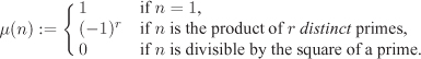
The Möbius function
It follows that μ(n) ≠ 0 if and only if n is square-free. |
Lemma 2.6.
|
For
where Proof The result follows immediately for n = 1. For n > 1, write |
Lemma 2.7. Möbius inversion formula
|
Let f and g be maps from
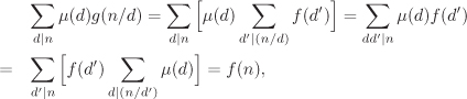
Proof To prove the additive formula we note that
where the last equality follows from Lemma 2.6. The multiplicative formula can be proved similarly. |
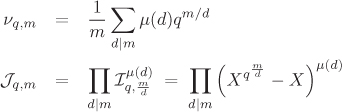
Let us denote by νq,m the number of monic irreducible polynomials in ![]() of degree m and by
of degree m and by ![]() the product of all monic irreducible polynomials in
the product of all monic irreducible polynomials in ![]() of degree m. By Theorem 2.40, we have
of degree m. By Theorem 2.40, we have ![]() and
and ![]() . Applications of the Möbius inversion formula then yield the following formulas:
. Applications of the Möbius inversion formula then yield the following formulas:
Equation 2.4
If p1, . . . , pr are all the prime divisors of m (not necessarily all distinct), Equation (2.4) together with the observation that μ(n) ≥ –1 for all ![]() imply that
imply that ![]() But each pi ≥ 2, so that m ≥ 2r, and hence
But each pi ≥ 2, so that m ≥ 2r, and hence ![]() . We, therefore, have an independent proof of the second statement in Corollary 2.17. Moreover, for practical values of q and m we have the good approximation:
. We, therefore, have an independent proof of the second statement in Corollary 2.17. Moreover, for practical values of q and m we have the good approximation:
Equation 2.5
![]()
Since the total number of monic polynomials of degree m in Fq[X] is qm, a randomly chosen monic polynomial in ![]() of degree m has an approximate probability of 1/m for being irreducible, that is, one expects to get an irreducible polynomial of degree m, after O(m) random monic polynomials are picked up from
of degree m has an approximate probability of 1/m for being irreducible, that is, one expects to get an irreducible polynomial of degree m, after O(m) random monic polynomials are picked up from ![]() . These observations have an important bearing for devising efficient algorithms for finding irreducible polynomials over finite fields. (See Chapter 3.)
. These observations have an important bearing for devising efficient algorithms for finding irreducible polynomials over finite fields. (See Chapter 3.)
The conjugates of ![]() over
over ![]() are αqi,
are αqi, ![]() . It is interesting to look at the sum and the product of the conjugates of α. By Corollary 2.18,
. It is interesting to look at the sum and the product of the conjugates of α. By Corollary 2.18, ![]() for some
for some ![]() . Since
. Since ![]() , the elements
, the elements ![]() and
and ![]() belong to
belong to ![]() . Since αqd = α, for any (positive) integral multiple δ of d, the sum
. Since αqd = α, for any (positive) integral multiple δ of d, the sum ![]() and the product
and the product ![]() are elements of
are elements of ![]() too.
too.
Definition 2.59.
|
Let
and the norm of α over
In view of the preceding discussion, the trace and norm of α are elements of |
The trace and norm functions play an important role in the theory of finite fields. See Exercise 2.86 for some elementary properties of these functions.
2.9.3. Representation of Finite Fields
![]() is a vector space of dimension m over
is a vector space of dimension m over ![]() . Let β0, . . . , βm–1 be an
. Let β0, . . . , βm–1 be an ![]() -basis of
-basis of ![]() . Each element
. Each element ![]() has a unique representation a = a0β0 + · · · + am–1βm–1 with each
has a unique representation a = a0β0 + · · · + am–1βm–1 with each ![]() . Therefore, if we have a representation of the elements of
. Therefore, if we have a representation of the elements of ![]() , we can also represent the elements of
, we can also represent the elements of ![]() . Thus elements of any finite field can be represented, if we have representations of elements of prime fields. But the set {0, 1, . . . , p – 1} under the modulo p arithmetic represents
. Thus elements of any finite field can be represented, if we have representations of elements of prime fields. But the set {0, 1, . . . , p – 1} under the modulo p arithmetic represents ![]() .
.
So our problem reduces to selecting suitable bases β0, . . . , βm–1 of ![]() over
over ![]() . In order to illustrate how we can do that, let us choose a priori a fixed monic irreducible polynomial
. In order to illustrate how we can do that, let us choose a priori a fixed monic irreducible polynomial ![]() with deg f = m. We then represent
with deg f = m. We then represent ![]() , where α (the residue class of X) is a root of f in
, where α (the residue class of X) is a root of f in ![]() . The elements
. The elements ![]() are linearly independent over
are linearly independent over ![]() , since otherwise we would have a non-zero polynomial of degree less than m, of which α is a root. The
, since otherwise we would have a non-zero polynomial of degree less than m, of which α is a root. The ![]() -basis 1, α, . . . , αm–1 of
-basis 1, α, . . . , αm–1 of ![]() is called a polynomial basis (with respect to the defining polynomial f). The elements of
is called a polynomial basis (with respect to the defining polynomial f). The elements of ![]() are then polynomials of degrees < m. The arithmetic in
are then polynomials of degrees < m. The arithmetic in ![]() is carried out as the polynomial arithmetic of
is carried out as the polynomial arithmetic of ![]() modulo the irreducible polynomial f.
modulo the irreducible polynomial f.
Example 2.19.
|
Polynomial bases are most common in finite field implementations. Some other types of bases also deserve specific mention in this context.
Definition 2.60.
It can be shown that normal bases exist for all finite extensions ![]() . It can even be shown that primitive normal bases also do exist for all such extensions.
. It can even be shown that primitive normal bases also do exist for all such extensions.
Example 2.20.
|
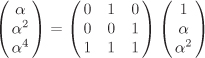
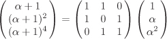
Consider the representation of
with the 3×3 transformation matrix having determinant 1 modulo 2. Thus α is a normal element of On the other hand, α + 1 is not a normal element of
with the transformation matrix having determinant zero modulo 2. |
Computations over finite fields often call for exponentiations of elements a = a0β0 + · · · + am–1βm–1. If βi = αqi, i = 0, . . . , m – 1, construct a normal basis, ![]() , since αqm = α and
, since αqm = α and ![]() for each i. Thus the coefficients of aq (in the representation under the given normal basis) is obtained simply by cyclically shifting the coefficients a0, . . . , am–1 in the representation of a. This leads to a considerable saving of time. In particular, this trick becomes most meaningful for q = 2 (a case of high importance in cryptography).
for each i. Thus the coefficients of aq (in the representation under the given normal basis) is obtained simply by cyclically shifting the coefficients a0, . . . , am–1 in the representation of a. This leads to a considerable saving of time. In particular, this trick becomes most meaningful for q = 2 (a case of high importance in cryptography).
Now that exponentiations become cheaper with normal bases, one should not let the common operations (addition and multiplication) turn significantly slower. The sum of a = a0β0 + · · · + am–1βm–1 and b = b0β0 + · · · + bm–1βm–1 continues to remain as easy as in the case of a polynomial basis, namely, a + b = (a0 + b0)β0 + · · · + (am–1 + bm–1)βm–1, where each ai + bi is calculated in ![]() . However, computing the product ab introduces difficulty. In particular, it requires the representation of βiβj, 0 ≤ i, j ≤ m – 1, in the basis β0, . . . , βm–1, say,
. However, computing the product ab introduces difficulty. In particular, it requires the representation of βiβj, 0 ≤ i, j ≤ m – 1, in the basis β0, . . . , βm–1, say, ![]() . For i ≤ j, we have
. For i ≤ j, we have ![]() . It is thus sufficient to look only at the coefficients
. It is thus sufficient to look only at the coefficients ![]() , 0 ≤ j, k ≤ m – 1. We denote by Cα the number of non-zero
, 0 ≤ j, k ≤ m – 1. We denote by Cα the number of non-zero ![]() . From practical considerations (for example, for hardware implementations), Cα should be as small as possible. For q = 2, one can show that 2m – 1 ≤ Cα ≤ m2. If, for this special case, Cα = 2m – 1, the normal basis α, αq, . . . , αqm–1 is called an optimal normal basis. Unlike normal (or primitive normal) bases, optimal normal bases do not exist for all values of
. From practical considerations (for example, for hardware implementations), Cα should be as small as possible. For q = 2, one can show that 2m – 1 ≤ Cα ≤ m2. If, for this special case, Cα = 2m – 1, the normal basis α, αq, . . . , αqm–1 is called an optimal normal basis. Unlike normal (or primitive normal) bases, optimal normal bases do not exist for all values of ![]() .
.
We finally mention another representation of elements of a finite field ![]() , that does not depend on the vector space representation discussed so far, but which is based on the fact that the group
, that does not depend on the vector space representation discussed so far, but which is based on the fact that the group ![]() is cyclic. If we are given a primitive element (that is, a generator) γ of
is cyclic. If we are given a primitive element (that is, a generator) γ of ![]() , then the elements of
, then the elements of ![]() are 0, 1 = γ0, γ, . . . , γq–2. Multiplication and exponentiation become easy with this representation, since 0 · a = 0 for all
are 0, 1 = γ0, γ, . . . , γq–2. Multiplication and exponentiation become easy with this representation, since 0 · a = 0 for all ![]() , whereas γi · γj = γk with k ≡ i + j (mod q – 1). Unfortunately, this representation provides no clue on how to compute γi + γj. One possibility is to store a table consisting of the values zk satisfying 1 + γk = γzk for all k = 0, . . . , q – 2 (with γk ≠ –1), so that for i ≤ j one can compute γi + γj = γi(1 + γj–i) = γiγzj–i = γl, where l ≡ i + zj–i (mod q – 1). Such a table is called Zech’s logarithm table, can be maintained for small values of q and may facilitate computations in extensions
, whereas γi · γj = γk with k ≡ i + j (mod q – 1). Unfortunately, this representation provides no clue on how to compute γi + γj. One possibility is to store a table consisting of the values zk satisfying 1 + γk = γzk for all k = 0, . . . , q – 2 (with γk ≠ –1), so that for i ≤ j one can compute γi + γj = γi(1 + γj–i) = γiγzj–i = γl, where l ≡ i + zj–i (mod q – 1). Such a table is called Zech’s logarithm table, can be maintained for small values of q and may facilitate computations in extensions ![]() . But if q is large (or more correctly if p is large, where q = pn), this representation of elements of
. But if q is large (or more correctly if p is large, where q = pn), this representation of elements of ![]() is not practical nor often feasible. Another difficulty of this representation is that it calls for a primitive element γ. If q is large and the integer factorization of q – 1 is not provided, there are no efficient methods known for finding such an element or even for checking if a given element is primitive.
is not practical nor often feasible. Another difficulty of this representation is that it calls for a primitive element γ. If q is large and the integer factorization of q – 1 is not provided, there are no efficient methods known for finding such an element or even for checking if a given element is primitive.
Example 2.21.
|
Consider the representation of |
| k | γk | 1 + γk | zk |
|---|---|---|---|
| 0 | 1 | 2 | 4 |
| 1 | β + 1 | β + 2 | 7 |
| 2 | 2β | 2β + 1 | 3 |
| 3 | 2β + 1 | 2β + 2 | 5 |
| 4 | 2 | 0 | – |
| 5 | 2β + 2 | 2β | 2 |
| 6 | β | β + 1 | 1 |
| 7 | β + 2 | β | 6 |
Exercise Set 2.9
| 2.80 | Let F be a field (not necessarily finite) of characteristic |
| 2.81 | Let
|
| 2.82 | Let |
| 2.83 | Write the addition and multiplication tables of (some representations of) the fields |
| 2.84 | Let K be a field (not necessarily finite or of positive characteristic).
|
| 2.85 | In this exercise, one studies the arithmetic in the finite field |
| 2.86 | Let F ⊆ K ⊆ L be finite extensions of finite fields with [L : K] = s. Let α,
|
| 2.87 | Let
|
| 2.88 | Let K and L be as in Exercise 2.87 and let |
| 2.89 | Let K and L be as in Exercise 2.87. Two K-bases (β0, . . . , βm–1) and (γ0, . . . , γm–1) of L are called dual or complementary, if TrL|K(βiγj) = δij.[10] Show that every K-basis of L has a unique dual basis.
|
| 2.90 | Prove that every finite extension of finite fields is Galois. [H] |
| 2.91 | For the extension |
| 2.92 | Let
|
| 2.93 | Consider the representation of |
| 2.94 | Show that the number of (ordered) (qm – 1)(qm – q)(qm – q2) · · ·(qm – qm – 1). |