
23
RETURNS TO DAMAGE AND DAMAGES TO RETURN
23.1 INTRODUCTION
Chapter 21 has discussed the two disposability concepts under a possible occurrence of “undesirable congestion (UC),” due to a capacity limit in part or all of a whole production facility, and another possible occurrence of “desirable congestion (DC)” due to eco‐technology innovation. In this chapter, technology innovation contains wide implications regarding not only engineering contributions but also managerial challenges (e,g., a fuel mix shift from coal to natural gas or renewable energy for generation).
The underlying philosophy of this book is that we may overcome our current difficulty on the global warming and climate change by combining technology development with managerial challenges. It is believed that the global climate issue, influencing all over the world, can be solved by engineering capabilities and natural science that are equipped with managerial and economic wisdoms in social science. This chapter documents an analytical rationale regarding how DEA can serve as an empirical basis for connecting among such different capabilities in engineering, natural and social sciences.
As an extension of Chapters 20 and 21, the purpose of this chapter is to discuss UC under natural disposability and DC under managerial disposability, along with their linkages to returns to damage (RTD) and damages to return (DTR). This chapter also equips DEA with an analytical capability of “explorative analysis” for multiplier restriction, as discussed in Chapter 22, to improve the measurement reliability on RTD under UC and DTR under DC. After theoretically discussing our research direction, this chapter documents the practicality of the proposed approach by applying it to Chinese energy assessment and regional economic planning. The proposed application examines China’s municipalities and provinces in terms of their economic and environmental developments.
The remainder of this chapter is organized as follows: Section 23.2 reviews economic concepts related to the occurrence of congestion. Section 23.3 describes these concepts with congestion under natural disposability. Section 23.4 shifts our discussion to another type of congestion under managerial disposability. Section 23.5 applies the proposed approach to discuss Chinese regional development and energy planning. Section 23.6 summarizes this chapter.
23.2 CONGESTION, RETURNS TO DAMAGE AND DAMAGES TO RETURN
23.2.1 Undesirable Congestion (UC) and Desirable Congestion (DC)
As discussed in Chapter 21, the occurrence of UC is a widely observed phenomenon in which inefficiency is identified in such a manner that an increase in some input(s) decreases some desirable output(s), without worsening other production factors, including undesirable output(s). That is an undesirable phenomenon. The straightforward expectation is that an increase in inputs leads to an increase in some components of desirable and undesirable output vectors. Such an occurrence of UC may be found in many economic activities, including business in energy sectors. See Chapter 9 that provides an illustrative example of UC in the electric power industry.
Returning to Chapter 21, we conceptually retreat our description on a possible occurrence of congestion, then connecting it to RTD and DTR. To explain the conceptual connection, this chapter presents Figure 23.1, originated from Figure 21.1. The left‐hand side of the figure exhibits the desirable output (g) on the vertical axis and the undesirable output (b) on the horizontal axis. The opposite case is found in the right‐hand side of the figure. For our visual convenience, Figure 23.1 considers only a single component of the three production factors. It is easily extendable to their multiple components in the mathematical formulations proposed in this chapter. The convex curve depicted in the figure indicates the relationship between two production factors.
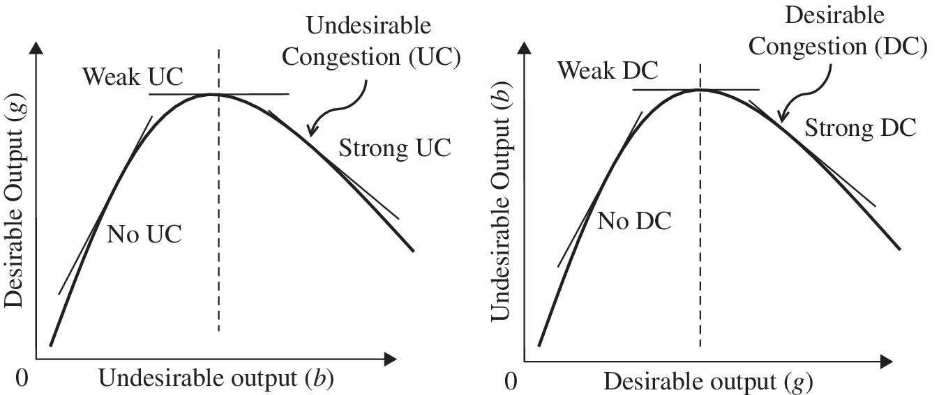
FIGURE 23.1 UC and DC (a) See Figure 21.1. Figure 23.1 changes Figure 21.1 by a smooth curve for our visual convenience and pays attention to the bottom of Figure 21.1, that is, a visual description of UC and DC. (b) For our visual convenience, part of input x is not shown in this figure (see Figure 21.1). For example, on the left‐hand side of Figure 23.1, the supporting hyperplane visually specifies the shape of the production curve and the possible occurrence of UC between desirable output (g) and undesirable output (b). A negative slope indicates the occurrence of UC, so being considered as “strong UC.” The occurrence of strong UC implies that enlarged input (x) increases undesirable output (b) and decreases the desirable output vector (g), as visually specified by the negative slope of the supporting line. In contrast, a positive slope implies an opposite case (i.e., no congestion), so being referred to as “no UC.” When the slope of a supporting hyperplane is zero, this chapter considers it as “weak UC,” being between strong UC and no UC. See Chapter 21, which explains this as the starting position of UC. The visual description on UC is extendable to a description on DC, or eco‐technology innovation for pollution reduction, as found on the right‐hand side of the figure. The three categories of DC include no (a positive slope), weak (a zero slope) and strong (a negative slope). (c) The occurrence of UC, or a capacity limit, becomes a serious problem in energy sectors so that it is necessary for us to identify such an occurrence in discussing energy policy. Meanwhile, the occurrence of DC, or eco‐technology innovation, may be more important than UC in terms of environmental protection and assessment because it is necessary for us to reduce the level of various types of pollution. (d) For our visual description, the figure uses a smooth curve to express the relationship between two production factors. The figure also depicts a single component of the three production factors. All the DEA formulations proposed in this chapter can handle their multiple components.
On the left‐hand side of Figure 23.1, a supporting line visually specifies the shape of a production curve and a possible occurrence of UC between g and b. For example, a negative slope indicates an occurrence of UC, so being considered as “strong UC,” as discussed in Chapter 21. An occurrence of strong UC implies that an enlarged input (x), not listed in Figure 23.1 for our visual description, increases an undesirable output (b) but decreases a desirable output (g). In contrast, a positive slope implies an opposite case (i.e., no congestion), so being referred to as “no UC.” If the slope of a supporting line is zero, this chapter considers it as “weak UC,” so being between strong UC and no UC.
The right‐hand side of Figure 23.1 visually specifies the three categories (i.e., no, weak and strong) of DC whose analytical implications are directly obtained from UC, but different implications. For a description for such a difference between UC and DC, it is necessary for us to exchange between the horizontal (b to g) and vertical (g to b) coordinates from UC, as found on the right‐hand side of Figure 23.1. See Chapter 21 for an illustrative example on UC under natural disposability. See also Chapter 22 for a detailed description on how to measure MRT and RSU among production factors, with a possible occurrence of DC, under managerial disposability.
23.2.2 Returns to Damage (RTD) under Undesirable Congestion (UC)
Figure 23.2 visually specifies the visual relationship among the three types of supporting hyperplane on a production and pollution possibility set. They are closely associated with the three types of UC, which are classified into “no,” “weak” and “strong” UC. As mentioned previously, an occurrence of UC becomes a serious difficulty in the operation of energy sectors. See Chapter 9 for an illustrative example of such a difficulty in the electric power industry.
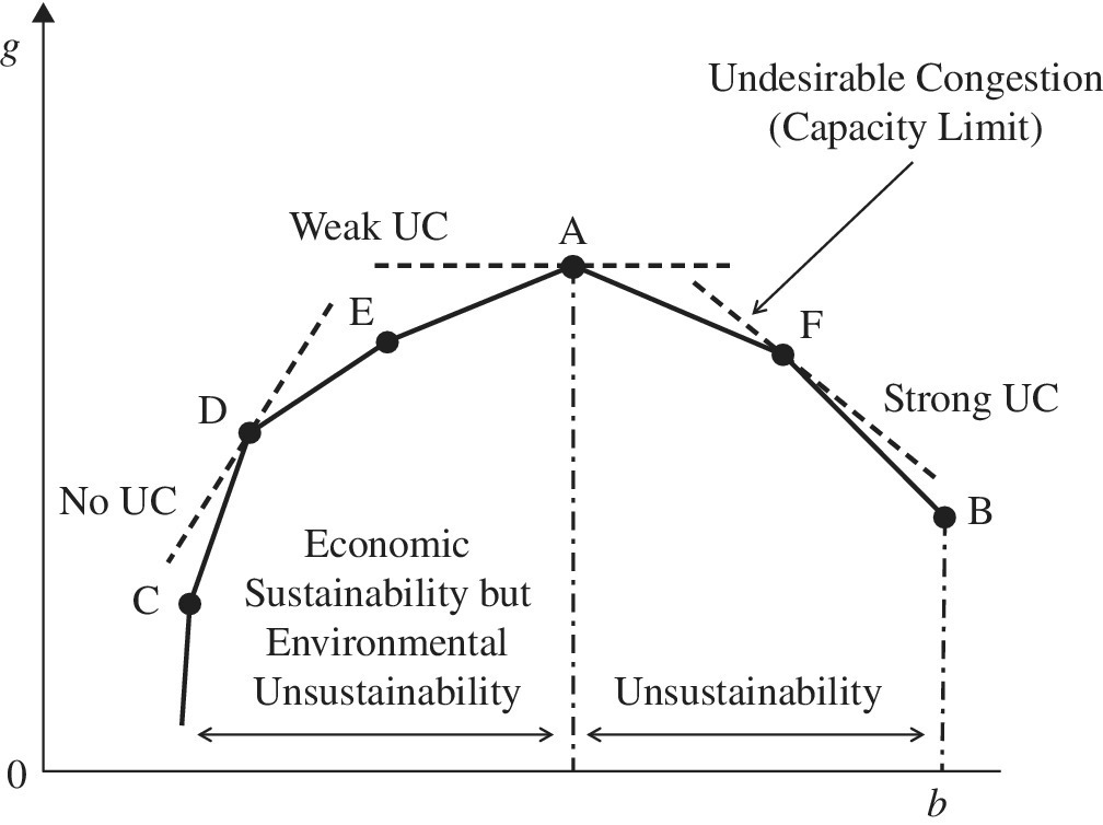
FIGURE 23.2 Undesirable Congestion (UC) (a) See Figure 21.2. (b) The figure visually specifies the relationship between the supporting hyperplane and the production and pollution possibility set. The types of UC include “no,” “weak” and “strong”. No UC is found at D, weak UC is found at A and strong UC is found on F. The occurrence of strong UC is identified by negative RTD if the three production factors have a single component, as depicted in the figure. (c) The figure does not incorporate the input (x) for our visual convenience. Hence, each dotted line can be considered as a supporting hyperplane.
Figure 23.3 visually discusses the three types of RTD, including “positive,” “no” and “negative” RTD. An efficiency frontier consists of the six DMUs ({C}–{D}–{E}–{A}–{F}–{B}). Positive RTD, corresponding to no UC, is further separated into IRTD on {C}, CRTD on {D}, and DRTD on {E}. No RTD is found on {A}, corresponding to weak UC, and negative RTD is found on {F}, corresponding to strong UC.
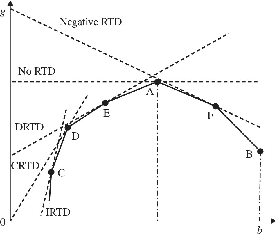
FIGURE 23.3 Returns to damage (RTD) (a) IRTD: Increasing RTD, CRTD: constant RTD and DRTD: decreasing RTD in the case of a desirable output (g) and undesirable output (b), all of which belong to “positive RTD.” In addition, there are no RTD and negative RTD. The negative RTD indicates an occurrence of strong UC due to a capacity limit in part or all of a whole production system. (b) A use of scale elasticity for RTD classification indicates that dg/db becomes zero on {A} and negative on {F}, where d stands for a derivative of a functional form between two components. The derivative mathematically indicates the slope of a supporting hyperplane. The other three points ({C}, {D} and {E}) have a positive slope. Thus, Figure 23.3 indicates a mathematical linkage between strong UC and negative RTD in the case of a single component of the three production factors. The case of multiple components is discussed by the proposed formulations for DEA environmental assessment in this chapter.
Here, it is important to note that a use of point elasticity for RTD classification indicates that dg/db becomes zero on {A} and negative on {F}, where d stands for a derivative of a functional form that mathematically expresses the slope of a supporting hyperplane. The other three points {C, D and E} have a positive slope of the supporting hyperplane. Thus, Figure 23.3 indicates a mathematical linkage between strong UC and negative RTD. Such a linkage will be mathematically explored in this chapter. The identification of negative RTD is important for all industries, including energy sectors, because it indicates an occurrence of strong UC, or a capacity limit in part or all of a whole production system.
23.2.3 Damages to Return (DTR) under Desirable Congestion (DC)
Shifting our description from UC to DC, Figure 23.4 depicts a possible occurrence of DC on a production and pollution possibility set between a single desirable output (g) on the horizontal axis and a single undesirable output (b) on the vertical axis. Figure 23.4 incorporates the condition of variable DTR. As depicted in Figure 23.4, DC is classified into three categories, including no DC on {D}, weak DC on {A} and strong DC on {F}. Figure 23.5 visually specifies the relationship between a supporting hyperplane and the five types of DTR in which positive DTR is classified into three categories into increasing DTR (IDTR) on {C}, constant DTR (CDTR) on {D}, and decreasing DTR (DDTR) on {E} in addition to no DTR on {A} and negative DTR on {F}.
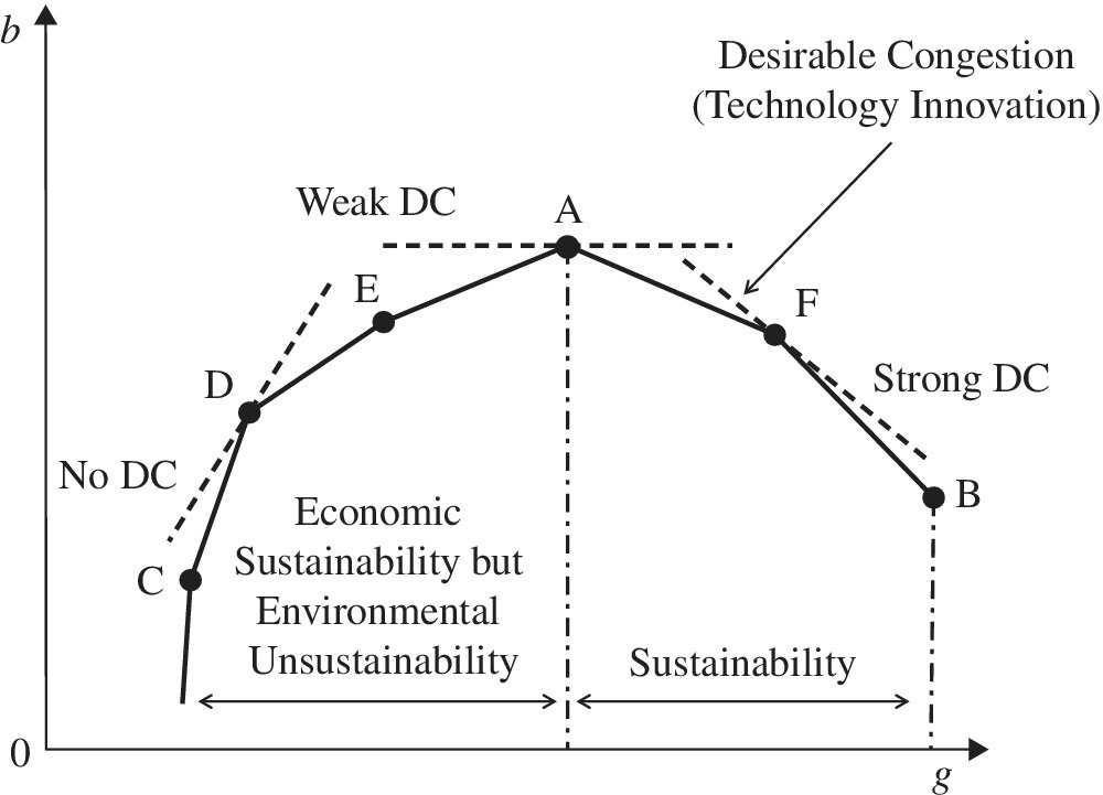
FIGURE 23.4 Desirable congestion (DC) (a) See Figure 21.3. (b) Figure 23.4 visually specifies the relationship between a supporting hyperplane and the types of DC, including “no,” “weak” and “strong” DC. No DC is found on {D}, weak DC is found on {A}. Strong DC occurs on {F} and such an occurrence may be identified by negative DTR if the three production factors have a single component. (c) An important feature of Figures 23.4 and 23.5 is that they have an assumption of byproducts. That is, undesirable outputs are byproducts of the desirable outputs. Hence, the figures have a convex form to express efficiency frontiers. Without this assumption, they should be structured by a concave form to express an efficiency frontier for undesirable outputs.
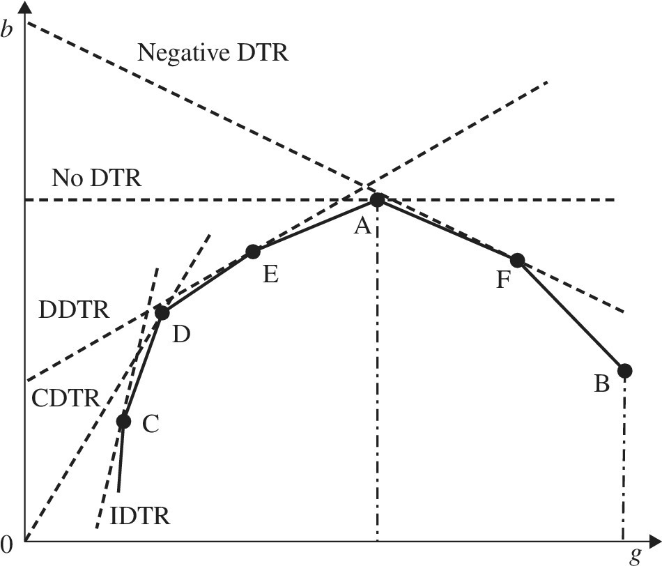
FIGURE 23.5 Damages to return (DTR) (a) IDTR: Increasing DTR, CDTR: constant DTR and DDTR: decreasing DTR in the case of an undesirable output (b) and desirable output (g). In addition, there is no DTR and negative DTR. A negative DTR indicates the occurrence of DC due to eco‐technology innovation for reducing the amount of undesirable outputs.
An important feature of Figures 23.4 and 23.5 is that they have an assumption on “byproducts” between b and g. That is, “undesirable outputs are byproducts of desirable outputs.” Hence, Figures 23.4 and 23.5 have a convex form to express an efficiency frontier. Without the assumption, an efficiency frontier for undesirable output should be structured by a concave form because the less undesirable outputs are the better in environmental assessment. See Figure 15.6, which provided a visual description on the convex and concave relationships in the three production factors. In addition, it visually discussed a rationale regarding why DEA environmental assessment is much more complicated and difficult than a conventional use of DEA. It is true that the only difference between the three production components is the existence of undesirable outputs among the production factors. However, such a difference makes the environmental assessment conceptually and analytically very different from the original use of DEA.
In Figure 23.5, the conventional use of scale elasticity for DTR classification indicates that db/dg becomes zero on {A} and negative on {F}. The derivative becomes positive at the other points ({C}, {D} and {E}). Thus, Figures 23.4 and 23.5 indicate a mathematical linkage between strong DC and negative DTR in the case that the three production factors have a single component. The visual description is extendable to the case of multiple components in the proposed formulations for DEA environmental assessment.
23.2.4 Possible Occurrence of Undesirable Congestion (UC) and Desirable Congestion (DC)
The possible occurrences of UC and DC are expressed by the following production and pollution set under the two disposability concepts:

and

Equation (23.1) incorporates a possible occurrence of UC under natural (N) disposability. Meanwhile, Equation (23.2) incorporates a possible occurrence of DC under managerial (M) disposability. The difference between the two equations can be found on the allocation of equality on desirable or undesirable outputs. Note that equality is formulated by dropping slacks in the proposed formulations. In contrast, inequality is formulated by maintaining slacks in the formulations.
Figure 23.6 visually describes a computational flow from the two disposability concepts to the measurement of RTD under natural disposability and that of DTR under managerial disposability.
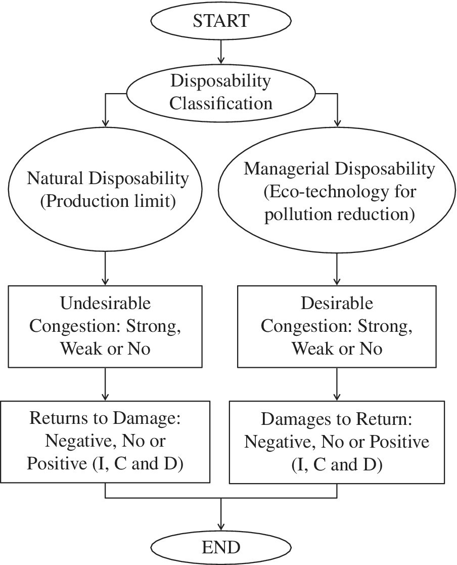
FIGURE 23.6 Computational flow from disposability to RTD and DTR (a) This figure visually describes the computational flow from the two disposability concepts to RTD under natural disposability and DTR under managerial disposability. (b) The possible occurrence of undesirable congestion is measured under natural disposability by assigning equality to the undesirable output (B). The occurrence indicates a technology limit on part or all of a whole production capability. (c) The possible occurrence of desirable congestion is measured under managerial disposability by assigning equality to the desirable output (G). The occurrence indicates an opportunity to reduce the amount of undesirable outputs by eco‐technology. (d) Strong, weak or no UC correspond to negative, no or positive RTD, respectively, in the case of a single component of three production factors. The UC is a necessary condition of RTD in the case of multiple components in the three production factors. (d) Strong, weak or no DC corresponds to negative, no or positive DTR, respectively, in the case of a single component of three production factors. The DC is a necessary condition of DTR in the case of multiple components in the three production factors. (e) I, C and D indicate increasing, constant and decreasing.
23.3 CONGESTION IDENTIFICATION UNDER NATURAL DISPOSABILITY
23.3.1 Possible Occurrence of Undesirable Congestion (UC)
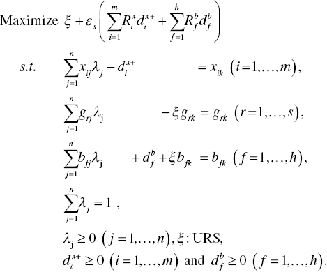
As depicted on the left‐hand side of Figure 23.6, this chapter can identify the possible occurrence of UC under natural disposability. To examine the occurrence, this chapter uses the following model that maintains equality constraints (so, no slack variable) on undesirable outputs, which is first specified in Model (21.3):
See a description on variables used in Model (21.3). Model (23.3) drops slack variables related to undesirable outputs (B) so that they are considered as equality constraints. The other constraints regarding inputs and desirable outputs are considered as inequality because they have slack variables in Model (23.3).
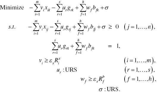
Model (23.3) has the following dual formulation:
See a description on variables used for Model (21.4). An important feature of Model (23.4) is that the dual variables (wf : URS for f = 1,…, h) are unrestricted in their signs because the constraints on undesirable outputs are expressed by equality (i.e., no slack) in Model (23.3). The dual variables are often referred to as multipliers as mentioned previously.
A unified efficiency measure of the k‐th DMU under natural disposability become
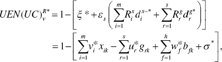
which incorporates the possible occurrence of UC, expressed by Equation (21.5). All variables used in Equation (23.5) are determined on the optimality of Models (23.3) and (23.4). The equation within the parenthesis, obtained from the optimal objective value of Models (23.3) and (23.4), indicates the level of unified inefficiency under natural disposability. The unified efficiency, or ![]() , is obtained by subtracting the level of inefficiency from unity as specified in Equation (23.5).
, is obtained by subtracting the level of inefficiency from unity as specified in Equation (23.5).
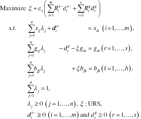
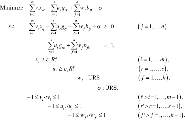
Explorative Analysis: An important advantage of Model (23.4) is that it can incorporate additional information in the form of side constraints for multiplier restrictions, as discussed in Chapter 22. For example, DEA environmental assessment usually divides the observation on each production factor by a factor average to avoid the case in which the data with a large magnitude dominates the other data with a small magnitude in the computation for assessment. Such a data adjustment is important for DEA to enhance the computational reliability. See Figure 22.3. As a result of multiplier restriction, all the observations used in this chapter are unit‐less, so indicating the importance of each production factor. The data adjustment makes it possible to incorporate additional side constraints on production factors in Model (23.4) as follows:
See Chapter 22, which refers to the multiplier restriction as “explorative analysis.” The analysis does not need any prior information so that it can avoid subjectivity in multiplier restriction, which is widely used in conventional DEA.
An important feature of the explorative analysis, used in Chapter 22, is that Equation (22.8) incorporates the following multiplier restrictions:
The multiplier restriction is important because we are interested in the relationship between desirable and undesirable outputs as well as that between undesirable outputs. Meanwhile, this chapter is concerned with the measurement of UEN, UC and RTD under natural disposability and UEM, DC and DTR under managerial disposability. Thus, it is necessary for us to prepare multiplier restrictions on all the three production factors, as specified in Equations (23.6), (23.7) and (23.8).
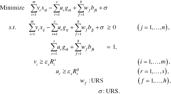
Model (23.4), equipped with Equations (23.6) to (23.8), becomes as follows:
The degree of ![]() on the k‐th DMU is determined by
on the k‐th DMU is determined by
where all the dual variables are identified on the optimality of Model (23.9). Equation (23.10) is different from Equation (23.5) because the side constraints in Equations (23.6) to (23.8) are additionally incorporated into Model (23.9). Therefore, Models (23.4) and (23.9) produce different ![]() measures.
measures.
After computing Model (23.9), a possible occurrence of UC is determined by the following rule under the assumption that Model (23.9) produces a unique optimal solution as discussed in Chapter 7 (i.e., unique projection and a unique reference set):
- If
 for some (at least one) f, then “strong UC” occurs on the k‐th DMU,
 - If
 for all f, then “no UC” occurs on the k‐th DMU and
 - In the others, including
 for some (at least one) f, then “weak UC” occurs on the k‐th DMU.
It is important to note that if ![]() for some f and
for some f and ![]() for the other f ′, then both strong UC and weak UC may coexist on the k‐th DMU. In the case, this chapter considers it as an occurrence of the strong UC on the DMU.
for the other f ′, then both strong UC and weak UC may coexist on the k‐th DMU. In the case, this chapter considers it as an occurrence of the strong UC on the DMU.
23.3.2 RTD Measurement under the Possible Occurrence of UC
Let the dual variables of the k‐th DMU, obtained from Model (23.9), be ![]() (i = 1, 2,…, m),
(i = 1, 2,…, m), ![]() (r = 1, 2,…, s),
(r = 1, 2,…, s), ![]() (f = 1, 2,…, h) and σ* on optimality. Then, the estimated supporting hyperplane on the k‐th DMU is expressed by
(f = 1, 2,…, h) and σ* on optimality. Then, the estimated supporting hyperplane on the k‐th DMU is expressed by
which is determined by ![]() , where RSk is a reference set for the k‐th DMU and
, where RSk is a reference set for the k‐th DMU and ![]() . See Proposition 21.1 in Chapter 21 that discusses mathematical implications regarding the supporting hyperplane. Note that Proposition 21.1 does not consider multiplier restriction, but Equation (23.11) has the explorative analysis. Both have the same mathematical equation, but they are different in terms of their analytical implications: congestion identification in Chapter 21 versus the determination of RTD and DTR in this chapter.
. See Proposition 21.1 in Chapter 21 that discusses mathematical implications regarding the supporting hyperplane. Note that Proposition 21.1 does not consider multiplier restriction, but Equation (23.11) has the explorative analysis. Both have the same mathematical equation, but they are different in terms of their analytical implications: congestion identification in Chapter 21 versus the determination of RTD and DTR in this chapter.
The degree (Dg) of RTD, or DgRTD, under a possible occurrence of UC, on the k‐th DMU is measured by
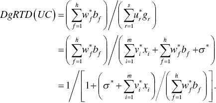
As mentioned previously, this chapter assumes that the Model (23.9) has both a unique projection of an inefficient DMU onto an efficiency frontier and a unique reference set for the DMU.
Following Equation (23.12), the type of RTD on the k‐th DMU is classified by the following rule on the k‐th DMU:
- Increasing RTD ↔ There exists an optimal solution of Model (23.9) that satisfies all
 (f = 1,…,h) and
 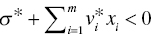 ,
, - Constant RTD ↔ There exists an optimal solution of Model (23.9) that satisfies all
 (f = 1,…,h) and
 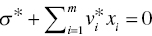 ,
, - Decreasing RTD ↔ There exists an optimal solution of Model (23.9) that satisfies all
 (f = 1,…,h) and
 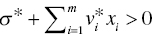 ,
, - Negative RTD ↔ There is an optimal solution of Model (23.9) that satisfies
 for at least one
  and
and - No RTD ↔ All other cases excluding (a) to (d).
Difference between UC and RTD: The type of UC is identified by the sign of dual variables (![]() ). The type of UC is classified into the three categories. Meanwhile, these measures related to RTD are determined by not only the sign of dual variables (
). The type of UC is classified into the three categories. Meanwhile, these measures related to RTD are determined by not only the sign of dual variables (![]() ) but also the sign of
) but also the sign of ![]() . The type of RTD is classified into the five categories. Figure 23.7 visually classifies the type of RTD under a possible occurrence of UC.
. The type of RTD is classified into the five categories. Figure 23.7 visually classifies the type of RTD under a possible occurrence of UC.
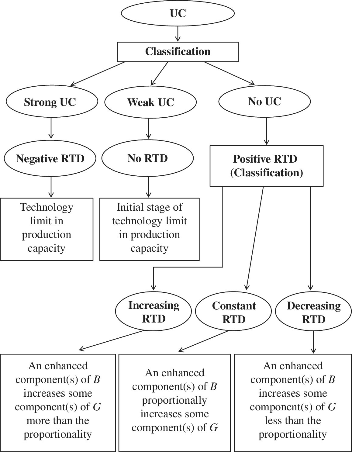
FIGURE 23.7 Returns to damage (RTD) under undesirable congestion (UC) (a) The increase in some component(s) of the input vector (X) increases the components of the other two production factors. The occurrence of UC is “undesirable” because some component(s) of the desirable output vector (G) decrease and those of the undesirable output vector (B) increase along with such a change of input vector. That is, the occurrence of UC is due to a capacity limit on part or whole in a production facility. (b) The occurrence and type of UC are identified by the sign of dual variables ( ). The type of UC is classified into three categories. Meanwhile, these measures related to RTD are determined by not only the sign of dual variables (
 ) but also the sign of
  . The type of RTD is classified into five categories.
At the end of this section, it is necessary to summarize three concerns related to Model (23.9) and Equation (23.12) as well as the proposed RTD classification. First, Model (23.9) assumes a unique solution, so implying no occurrence on multiple projections and multiple reference sets. Second, Equation (23.12) is effective on only efficient DMUs, not inefficient ones. In the case of inefficiency, Equation (23.12) needs to incorporate the projection onto an efficiency frontier by both adjusting an inefficiency score and eliminating slacks from the observed production factors, as discussed in Chapter 20. The multiplier restriction by the proposed explorative analysis is more influential, so effective, on the measurement of RTD and DTR than slack adjustment. Therefore, this chapter, like Chapter 22, does not provide a detailed description on slack adjustment. Finally, the type of RTD is determined by measuring the upper and lower bound of ![]() . The proposed approach is just an approximation method for the RTD measurement for our descriptive convenience. Thus, the proposed RTD measurement needs to be extended further by adjusting slacks under a possible occurrence of multiple solutions (e.g., multiple references and multiple projections). See Chapter 7 on how to handle such an occurrence of multiple solutions.
. The proposed approach is just an approximation method for the RTD measurement for our descriptive convenience. Thus, the proposed RTD measurement needs to be extended further by adjusting slacks under a possible occurrence of multiple solutions (e.g., multiple references and multiple projections). See Chapter 7 on how to handle such an occurrence of multiple solutions.
23.4 CONGESTION IDENTIFICATION UNDER MANAGERIAL DISPOSABILITY
23.4.1 Possible Occurrence of Desirable Congestion (DC)
As depicted on the right‐hand side of Figure 23.6, this chapter can identify an occurrence of DC under managerial disposability. To examine the occurrence, this chapter uses the following model, returning to Model (21.7), which maintains equality constraints (so, no slack variable) on desirable outputs, as specified in Equation (23.2):
Model (23.13) drops slack variables related to desirable outputs so that they are considered as equality constraints. The other groups of constraints on inputs and undesirable outputs have slacks so that they can be considered as inequality constraints.
Model (23.13) has the following dual formulation:
An important feature of Model (23.14) is that the dual variables (ur : URS for r = 1,…, s) are unrestricted in these signs because Model (23.13) does not have slacks related to desirable outputs.
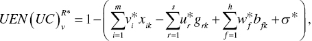
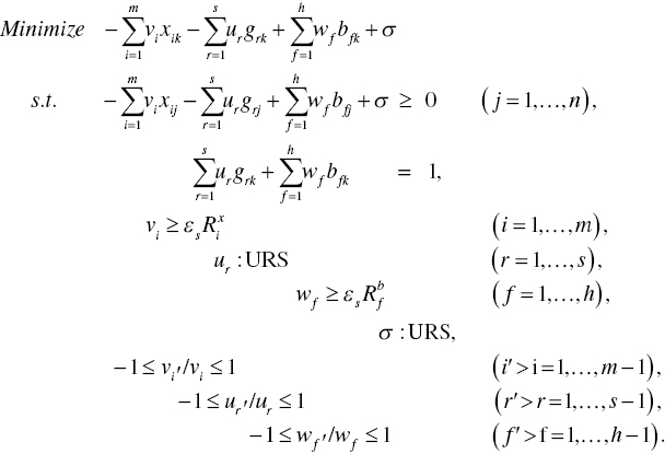
A unified efficiency score, or UEM(DC) of the k‐th DMU, with a possible occurrence of DC, under managerial disposability is determined by
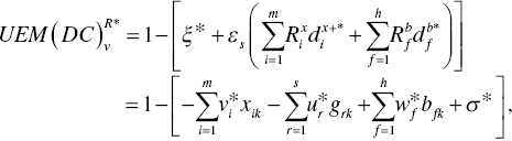
where all variables are determined on the optimality of Models (23.13) and (23.14). The equation within the parenthesis, obtained from the optimality of Models (23.13) and (23.14), indicates the level of unified inefficiency under managerial disposability. The unified efficiency is obtained by subtracting the level of inefficiency from unity.
As discussed on Model (23.9), Model (23.14) can incorporate additional information by explorative analysis that is formulated as follows:
The degree of ![]() is determined by
is determined by
where all the dual variables are identified on the optimality of Model (23.16). Equation (23.17) is different from Equation (23.15) because Model (23.16) incorporates the additional side constraints in Equations (23.6) to (23.8). Thus, Equations (23.15) and (23.17) produce different ![]() measures.
measures.
After solving Model (23.16), this chapter can identify the possible occurrence of DC, or eco‐technology innovation, by the following rule under the assumption on a unique optimal solution (i. e. unique projection and a unique reference set):
- If
 for some (at least one) r, then “strong DC” occurs on the k‐th DMU,
 - If
 for all r, then “no DC” occurs on the k‐th DMU and
 - In the others, including
 for some (at least one) r, then “weak DC” occurs on the k‐th DMU.
Note that if ![]() for some r and
for some r and ![]() for the other r′, then the weak and strong DCs coexist on the k‐th DMU. This study considers it as the strong DC, so indicating eco‐technology innovation on undesirable outputs. If
for the other r′, then the weak and strong DCs coexist on the k‐th DMU. This study considers it as the strong DC, so indicating eco‐technology innovation on undesirable outputs. If ![]() for all r. then it indicates the best case because an increase in any desirable output always decreases an amount of undesirable outputs. Meanwhile, if
for all r. then it indicates the best case because an increase in any desirable output always decreases an amount of undesirable outputs. Meanwhile, if ![]() is identified for some r, then it indicates that there is a chance to reduce an amount of undesirable output(s). Therefore, this chapter considers the second case as an occurrence of DC.
is identified for some r, then it indicates that there is a chance to reduce an amount of undesirable output(s). Therefore, this chapter considers the second case as an occurrence of DC.
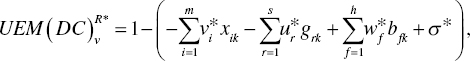
23.4.2 DTR Measurement under the Possible Occurrence of DC
Let the dual variables of the k‐th DMU, obtained from Model (23.16), be ![]() (i = 1, 2,…, m),
(i = 1, 2,…, m), ![]() (r = 1, 2,…, s),
(r = 1, 2,…, s), ![]() (f = 1, 2,…, h) and σ *. Then, an estimated supporting hyperplane on the k‐th DMU is specified by
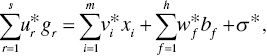
(f = 1, 2,…, h) and σ *. Then, an estimated supporting hyperplane on the k‐th DMU is specified by
The equation is characterized by ![]() , where RSk is a reference set of the k‐th DMU along with
, where RSk is a reference set of the k‐th DMU along with ![]() .
.
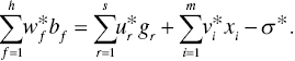
This chapter assumes that Model (23.16) has both a unique projection of an inefficient DMU onto an efficiency frontier and a unique reference set for the projected DMU. Then, the degree (Dg) of DTR, or DgDTR, is measured by
Consequently, the type of DTR is classified by the following rule on the k‐th DMU:
- Increasing DTR ↔ There is an optimal solution of Model (23.16) that satisfies all
 (r = 1,…, s) and
 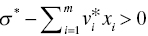 .
. - Constant DTR ↔ There exists an optimal solution of Model (23.16) that satisfies all
 (r = 1,…, s) and
 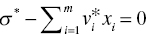 .
. - Decreasing DTR ↔ There is an optimal solution of Model (23.16) that satisfies all
 (r = 1,…, s) and
  .
. - Negative DTR ↔ There is an optimal solution of Model (23.16) that satisfies
 for at least one
  and
and - No DTR ↔ All other cases excluding (a) to (d).
All the concerns discussed for the measurement of RTD in Section 23.3.2 are applicable to DTR. However, it is important to note that the type of DTR is determined by measuring the upper and lower bounds of ![]() . The proposed approach for DTR is just an approximation method for the DTR measurement.
. The proposed approach for DTR is just an approximation method for the DTR measurement.
Difference between DC and DTR: The occurrence and type of DC are identified by the sign of dual variables (![]() ). The type of DC is classified into three categories. Meanwhile, these measures related to DTR are determined by not only the sign of dual variables (
). The type of DC is classified into three categories. Meanwhile, these measures related to DTR are determined by not only the sign of dual variables (![]() ) but also the sign of
) but also the sign of ![]() . The type of DTR is classified into five categories. Figure 23.8 visually describes an occurrence of DC and DTR classification.
. The type of DTR is classified into five categories. Figure 23.8 visually describes an occurrence of DC and DTR classification.
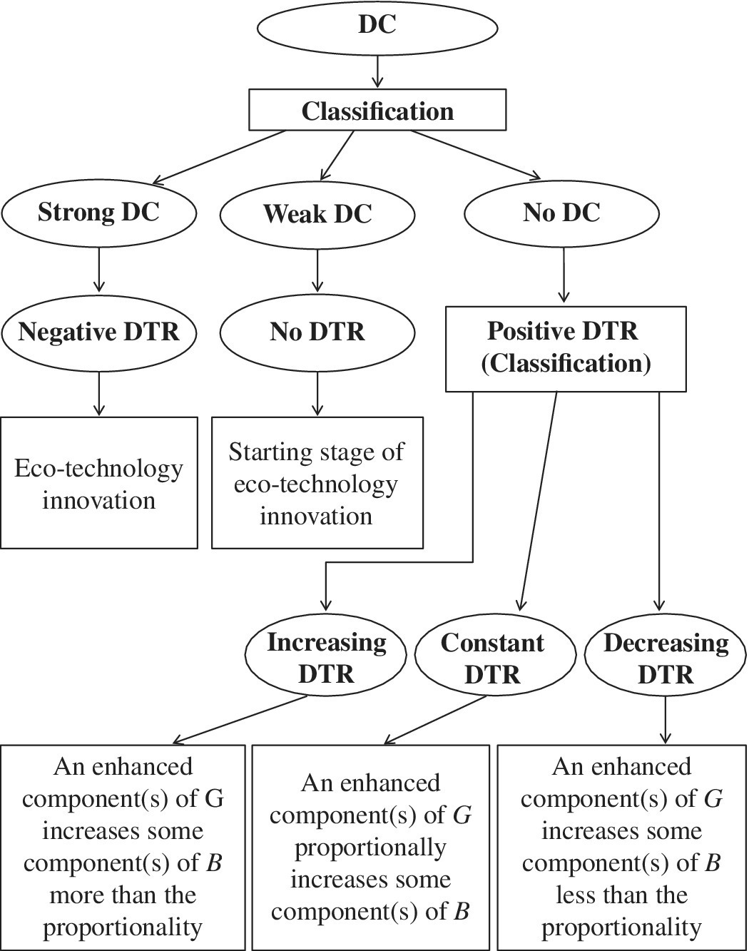
FIGURE 23.8 Damages to return (DTR) under desirable congestion (DC) (a) An increase in some component(s) of the input vector (X) increases the components of the other two production factors. The occurrence of DC is desirable because some component(s) of the desirable output vector (G) increase but those of the undesirable output vector (B) decrease along with such a change in input vector. That is an occurrence of DC. We look for such an occurrence by eco‐technology innovation in a broad sense, including managerial challenges. (b) The occurrence and type of DC are identified by the sign of dual variables ( ). The type of DC is classified into three categories. Meanwhile, these measures related to DTR are determined by not only the sign of dual variables (
 ), but also the sign of
  . The type of DTR is classified into five categories.
23.5 ENERGY AND SOCIAL SUSTAINABILITY IN CHINA
23.5.1 Data
This chapter presents a data set from the National Bureau of Statistics of the People’s Republic of China (http://www.stats.gov.cn/tjsj/). The National Bureau of Statistics provides a regional data set on energy, environment and other aspects of the whole country every year. Using the data set, this chapter examines 30 provinces of China, including four well‐developed municipalities directly under the control of central government (i.e., Beijing, Shanghai, Tianjin and Chongqing) but excluding Tibet, Hong Kong and Macau because of our limited data accessibility on these three regions during 2012.
We utilize four desirable outputs: Gross Regional Product (GRP), value‐added of the primary industry, the secondary industry and the tertiary industry; three undesirable outputs: PM10, SO2 and NO2; five inputs: investment in energy industry, coal consumption, oil consumption, natural gas consumption and electricity consumption. Descriptive Statistics are listed in Sueyoshi and Yuan (2016b).
Data Accessibility: The supplementary section of Sueyoshi and Yuan (2016b) lists the full data set used in this chapter.
It is important to note that the three undesirable outputs are not GHG emissions, rather SO2 and NO2, which are acid rain gases that produce much more serious damages than GHG. This chapter clearly understands that PM 2.5 has more serious impacts than PM 10 in terms of health damage on Chinese people. However, this chapter could not access any information on PM 2.5 during the observed annual period (2012).
To control for data magnitudes, this chapter further calculates a provincially adjusted index to be used in the proposed DEA models for all variables. The index of each factor is the ratio of the actual value divided by the average of each one. Note that this chapter sets εs = 0.0001 in the computation of the proposed DEA models.
23.5.2 Empirical Results
Table 23.1 lists the dual variables (multipliers), the degree of ![]() and the type of UC on thirty municipalities and provinces in 2012. The purpose of Table 23.1 is that this chapter needs to document how the proposed explorative analysis can change these measures. Model (23.4) is used for these computations. The model for
and the type of UC on thirty municipalities and provinces in 2012. The purpose of Table 23.1 is that this chapter needs to document how the proposed explorative analysis can change these measures. Model (23.4) is used for these computations. The model for ![]() has excluded the three groups of multiplier restrictions, or Equations (23.6) to (23.8). A problem found in Table 23.1 is that the magnitude of these dual variables is relatively large so that only Inner Mongolia becomes inefficient (0.8724). The others are all efficient. The type of UC is “strong” for all provinces. These results are unacceptable in this type of empirical study because it contains many efficient provinces. Further, the empirical results are unacceptable from the perspective of energy and economic planning for Chinese sustainability development because there is no difference among them and almost all are efficient. This indicates a methodological drawback of DEA environmental assessment. This type of difficulty may often occur in DEA and its applications for environmental assessment.
has excluded the three groups of multiplier restrictions, or Equations (23.6) to (23.8). A problem found in Table 23.1 is that the magnitude of these dual variables is relatively large so that only Inner Mongolia becomes inefficient (0.8724). The others are all efficient. The type of UC is “strong” for all provinces. These results are unacceptable in this type of empirical study because it contains many efficient provinces. Further, the empirical results are unacceptable from the perspective of energy and economic planning for Chinese sustainability development because there is no difference among them and almost all are efficient. This indicates a methodological drawback of DEA environmental assessment. This type of difficulty may often occur in DEA and its applications for environmental assessment.
TABLE 23.1 UEN(UC) and type of UC: Model (23.4)
(a) Source: Sueyoshi and Yuan (2016b). (b) w1 stands for the dual variable of PM10. w2 stands for the dual variable of SO2 and w3 stands for the dual variable of NO2. If ![]() for some (at least one) f, then “strong UC” occurs on the k‐th DMU; if
for some (at least one) f, then “strong UC” occurs on the k‐th DMU; if ![]() for all f, then “no UC” occurs on the k‐th DMU. In the others, including
for all f, then “no UC” occurs on the k‐th DMU. In the others, including ![]() for some (at least one) f, then “weak UC” occurs on the k‐th DMU. If
for some (at least one) f, then “weak UC” occurs on the k‐th DMU. If ![]() for some f and
for some f and ![]() for other fʹ, then both strong and weak UCs coexist on the k‐th DMU. In the case, this chapter considers the occurrence as strong UC. (c) Model (23.4) does not incorporate the proposed explorative analysis. Consequently, the dual variables are large in their magnitudes. In addition, most of municipalities and provinces are rated as unity in their unified efficiencies under natural disposability and strong undesirable congestion (UC). The results are unacceptable because this chapter is concerned with policy suggestions for Chinese regional economic and energy planning.
for other fʹ, then both strong and weak UCs coexist on the k‐th DMU. In the case, this chapter considers the occurrence as strong UC. (c) Model (23.4) does not incorporate the proposed explorative analysis. Consequently, the dual variables are large in their magnitudes. In addition, most of municipalities and provinces are rated as unity in their unified efficiencies under natural disposability and strong undesirable congestion (UC). The results are unacceptable because this chapter is concerned with policy suggestions for Chinese regional economic and energy planning.
| Province | w1 | w2 | w3 | σ | UEN(UC) | UC |
| Beijing | –67.0832 | –8.2505 | –55.5696 | 180.9354 | 1.0000 | Strong |
| Tianjin | –62.4183 | –132.3779 | 84.9027 | 169.7916 | 1.0000 | Strong |
| Hebei | 34.4745 | –194.2958 | 65.7054 | 194.4844 | 1.0000 | Strong |
| Shanxi | 68.9023 | –160.0109 | 160.0633 | 20.4058 | 1.0000 | Strong |
| Inner Mongolia | 0.8787 | –0.2406 | 0.1085 | –0.4814 | 0.8724 | Strong |
| Liaoning | 71.9875 | –210.5759 | 112.1153 | 124.0256 | 1.0000 | Strong |
| Jilin | 87.1350 | 14.4970 | –171.6050 | 37.2246 | 1.0000 | Strong |
| Heilongjiang | 84.4352 | –99.7433 | –122.1147 | 163.9192 | 1.0000 | Strong |
| Shanghai | 237.9280 | –51.9457 | –201.9009 | 41.2487 | 1.0000 | Strong |
| Jiangsu | –131.0119 | 7.2340 | –79.3795 | 314.9994 | 1.0000 | Strong |
| Zhejiang | 116.6050 | –100.2130 | –178.5735 | 224.9997 | 1.0000 | Strong |
| Anhui | –198.2258 | 73.5496 | 108.2929 | 97.3453 | 1.0000 | Strong |
| Fujian | –13.7631 | 181.0110 | –117.9729 | 41.7415 | 1.0000 | Strong |
| Jiangxi | 37.2990 | –131.1707 | 10.6483 | 116.1614 | 1.0000 | Strong |
| Shandong | –98.8847 | –112.3617 | 24.8536 | 301.4538 | 1.0000 | Strong |
| Henan | –37.4985 | –129.0649 | –28.9755 | 283.0348 | 1.0000 | Strong |
| Hubei | 20.3504 | 4.3239 | –156.9993 | 200.5690 | 1.0000 | Strong |
| Hunan | –72.0972 | –7.6075 | –106.3379 | 234.3867 | 1.0000 | Strong |
| Guangdong | 140.8545 | 11.6748 | –208.1419 | 184.8141 | 1.0000 | Strong |
| Guangxi | –41.9882 | 87.1230 | –71.2541 | 12.4540 | 1.0000 | Strong |
| Hainan | 61.0643 | 62.2186 | –94.0134 | –26.7372 | 1.0000 | Strong |
| Chongqing | –165.8771 | –33.5683 | 102.1901 | 44.9664 | 1.0000 | Strong |
| Sichuan | –185.8158 | 30.7800 | –12.9453 | 282.8272 | 1.0000 | Strong |
| Guizhou | –81.1661 | –59.7219 | 135.6327 | –22.3290 | 1.0000 | Strong |
| Yunnan | 404.0265 | –138.0444 | –225.1171 | –4.2690 | 1.0000 | Strong |
| Shaanxi | –265.8177 | –11.4641 | 118.9462 | 236.2667 | 1.0000 | Strong |
| Gansu | –135.2600 | –31.4009 | 194.0356 | 4.8144 | 1.0000 | Strong |
| Qinghai | –93.7301 | –82.1600 | 267.1938 | –19.5242 | 1.0000 | Strong |
| Ningxia | 83.9409 | –72.0011 | –17.4262 | –34.0242 | 1.0000 | Strong |
| Xinjiang | 266.7831 | –55.6519 | –248.3287 | –22.9935 | 1.0000 | Strong |
Table 23.2 lists the dual variables (multipliers), the degree of ![]() and the type of DC for the 30 municipalities and provinces in 2012. Table 23.2 also documents how the proposed multiplier restrictions can change these measures. Model (23.14) is used for these computations. The model for
and the type of DC for the 30 municipalities and provinces in 2012. Table 23.2 also documents how the proposed multiplier restrictions can change these measures. Model (23.14) is used for these computations. The model for ![]() does not utilize the three groups for explorative analysis, or Equations (23.6)–(23.8). The magnitude of these dual variables is relatively large so that Table 23.2 still contains many efficient municipalities and provinces in
does not utilize the three groups for explorative analysis, or Equations (23.6)–(23.8). The magnitude of these dual variables is relatively large so that Table 23.2 still contains many efficient municipalities and provinces in ![]() . Exceptions in these
. Exceptions in these ![]() measures are Jilin (0.8615) and Jiangxi (0.7947). All municipalities and provinces have strong DC. These results are also unacceptable from the perspective of China’s sustainability development. Thus, Tables 23.1 and 23.2 clearly indicate the necessity of explorative analysis in the classification of UC and DC. The difficulty identified in Tables 23.1 and 23.2 can be overcome by incorporating the proposed explorative analysis, or Equations (23.6) to (23.8), as formulated in Models (23.9) and (23.16).
measures are Jilin (0.8615) and Jiangxi (0.7947). All municipalities and provinces have strong DC. These results are also unacceptable from the perspective of China’s sustainability development. Thus, Tables 23.1 and 23.2 clearly indicate the necessity of explorative analysis in the classification of UC and DC. The difficulty identified in Tables 23.1 and 23.2 can be overcome by incorporating the proposed explorative analysis, or Equations (23.6) to (23.8), as formulated in Models (23.9) and (23.16).
TABLE 23.2 UEM(DC) and type of DC: Model (23.14)
(a) Source: Sueyoshi and Yuan (2016b). (b) u1 stands for the dual variable of GRP. u2 stands for the dual variable of value‐added of the primary industry. u3 stands for the dual variable of value‐added of the secondary industry. u4 stands for the dual variable of value‐added of the tertiary industry. If ![]() for some (at least one) r, then “strong DC” occurs on the k‐th DMU. If
for some (at least one) r, then “strong DC” occurs on the k‐th DMU. If ![]() for all r, then “no DC” occurs on the k‐th DMU. In the others, including
for all r, then “no DC” occurs on the k‐th DMU. In the others, including ![]() for some (at least one) f, then “weak DC” occurs on the k‐th DMU. If
for some (at least one) f, then “weak DC” occurs on the k‐th DMU. If ![]() for some r and
for some r and ![]() for other r′, then the weak and strong DCs coexist on the k‐th DMU. In this case, this study considers the occurrence as strong DC. (c) Model (23.14) does not incorporate the proposed multiplier restriction. Consequently, these dual variables are large in their magnitudes. All provinces, except Heilongjiang and Jiangxi, are rated as unity in their unified efficiency measures under managerial disposability and they are all under strong DC. The results are unacceptable in terms of Chinese regional economic and energy planning.
for other r′, then the weak and strong DCs coexist on the k‐th DMU. In this case, this study considers the occurrence as strong DC. (c) Model (23.14) does not incorporate the proposed multiplier restriction. Consequently, these dual variables are large in their magnitudes. All provinces, except Heilongjiang and Jiangxi, are rated as unity in their unified efficiency measures under managerial disposability and they are all under strong DC. The results are unacceptable in terms of Chinese regional economic and energy planning.
| Province | u1 | u2 | u3 | u4 | σ | UEM(DC) | DC |
| Beijing | –30.7337 | –21.7401 | –135.4404 | 22.5453 | 72.4647 | 1.0000 | Strong |
| Tianjin | –15.0532 | –220.4132 | 215.1855 | –190.9422 | 8.2407 | 1.0000 | Strong |
| Hebei | –58.3249 | 84.2157 | –150.9658 | –25.7218 | 91.9477 | 1.0000 | Strong |
| Shanxi | –46.9406 | –33.6323 | –68.2970 | –18.8360 | 69.9693 | 1.0000 | Strong |
| Inner Mongolia | –58.6732 | 6.6154 | –58.8331 | –72.3189 | 64.7705 | 1.0000 | Strong |
| Liaoning | –0.3693 | –89.0342 | 155.5847 | –225.2064 | –19.9005 | 1.0000 | Strong |
| Jilin | –15.0745 | 0.1319 | 12.0872 | 1.8615 | –1.2502 | 0.8615 | Strong |
| Heilongjiang | –28.2626 | 112.5519 | –315.6184 | 32.5089 | 98.0199 | 1.0000 | Strong |
| Shanghai | –30.3279 | –50.6093 | –59.9712 | –1.6165 | 21.0333 | 1.0000 | Strong |
| Jiangsu | –13.9364 | 6.0038 | 19.7134 | –58.6522 | 101.8990 | 1.0000 | Strong |
| Zhejiang | –26.7302 | –221.2135 | 309.0860 | –201.1764 | –28.0248 | 1.0000 | Strong |
| Anhui | 15.7277 | –14.6938 | 151.1975 | –348.3844 | –26.6403 | 1.0000 | Strong |
| Fujian | –7.5001 | –35.3934 | 93.7482 | –145.4879 | –26.9089 | 1.0000 | Strong |
| Jiangxi | 26.8480 | –2.5907 | –12.3890 | –11.7510 | –0.4537 | 0.7947 | Strong |
| Shandong | –27.2371 | 22.9688 | –40.1558 | –22.7104 | 52.3088 | 1.0000 | Strong |
| Henan | 10.6726 | 1.5341 | 97.7867 | –261.1320 | 99.8903 | 1.0000 | Strong |
| Hubei | 1.4970 | 1.4296 | –2.1370 | –1.2948 | 0.8822 | 1.0000 | Strong |
| Hunan | –28.0571 | 4.3695 | 11.1387 | 12.3020 | 1.1926 | 1.0000 | Strong |
| Guangdong | –12.1954 | –20.8928 | –23.0836 | 2.3836 | 30.3790 | 1.0000 | Strong |
| Guangxi | –91.2473 | 107.8889 | –134.0183 | –127.2700 | 32.9213 | 1.0000 | Strong |
| Hainan | –35.6506 | –33.7526 | –11.8598 | –69.0107 | –9.4207 | 1.0000 | Strong |
| Chongqing | –9.5122 | –213.8387 | 265.6208 | –229.2442 | 11.1692 | 1.0000 | Strong |
| Sichuan | –37.7014 | 12.6096 | –44.6575 | –42.2490 | 62.3629 | 1.0000 | Strong |
| Guizhou | –19.5151 | 28.8248 | –355.0989 | 45.3138 | 40.4201 | 1.0000 | Strong |
| Yunnan | –51.1983 | 68.7073 | –288.5694 | 5.0715 | 71.7098 | 1.0000 | Strong |
| Shaanxi | –35.4637 | –197.4817 | 389.7037 | –353.5435 | 13.7583 | 1.0000 | Strong |
| Gansu | –123.0311 | 21.9416 | –229.7992 | –138.5931 | –17.9110 | 1.0000 | Strong |
| Qinghai | –50.0142 | –108.3042 | –6.3172 | –115.2217 | 16.3682 | 1.0000 | Strong |
| Ningxia | –77.7710 | –102.4935 | –98.1680 | –76.9879 | –9.4704 | 1.0000 | Strong |
| Xinjiang | –48.3400 | 17.8205 | –168.7917 | –10.8003 | 109.0019 | 1.0000 | Strong |
Table 23.3 summarizes ![]() under the restriction and type of UC. Table 23.4 summarizes
under the restriction and type of UC. Table 23.4 summarizes ![]() under restriction and the type of DC. This chapter finds two important features in the two tables. One feature is that the number of efficient municipalities and provinces in the two tables reduces from those of Tables 23.1 and 23.2. More variations can be found in the type of UC of Table 23.3 and in the type of DC of Table 23.4. Thus, the comparison among Tables 23.3 and 23.4 indicates the importance of the proposed explorative analysis in terms of determining the type of UC and DC. Consequently, this chapter uses results from Tables 23.3 and 23.4, hereafter, for discussing Chinese energy planning and economic development.
under restriction and the type of DC. This chapter finds two important features in the two tables. One feature is that the number of efficient municipalities and provinces in the two tables reduces from those of Tables 23.1 and 23.2. More variations can be found in the type of UC of Table 23.3 and in the type of DC of Table 23.4. Thus, the comparison among Tables 23.3 and 23.4 indicates the importance of the proposed explorative analysis in terms of determining the type of UC and DC. Consequently, this chapter uses results from Tables 23.3 and 23.4, hereafter, for discussing Chinese energy planning and economic development.
TABLE 23.3 UEN(UC) and type of UC: Model (23.9)
(a) Source: Sueyoshi and Yuan (2016b). (b) w1 stands for the dual variable of PM10. w2 stands for the dual variable of SO2 and w3 stands for the dual variable of NO2. (c) If ![]() for some (at least one) f, then “strong UC” occurs on the k‐th DMU. If
for some (at least one) f, then “strong UC” occurs on the k‐th DMU. If ![]() for all f, then “no UC” occurs on the k‐th DMU. In the others, including
for all f, then “no UC” occurs on the k‐th DMU. In the others, including ![]() for some (at least one) f, then “weak UC” occurs on the k‐th DMU. If
for some (at least one) f, then “weak UC” occurs on the k‐th DMU. If ![]() for some f and
for some f and ![]() for the other f′, then both strong and weak UCs coexist on the k‐th DMU. In the case, this study considers the occurrence as strong UC. (d) Model (23.9) incorporates the proposed multiplier restriction. Consequently, these ratios between dual variables are between –1 and +1 in their magnitudes. The results on unified efficiency measures under natural disposability and the type of undesirable congestion (UC) are acceptable in terms of Chinese regional economic and energy planning.
for the other f′, then both strong and weak UCs coexist on the k‐th DMU. In the case, this study considers the occurrence as strong UC. (d) Model (23.9) incorporates the proposed multiplier restriction. Consequently, these ratios between dual variables are between –1 and +1 in their magnitudes. The results on unified efficiency measures under natural disposability and the type of undesirable congestion (UC) are acceptable in terms of Chinese regional economic and energy planning.
| Province | w1 | w2 | w3 | σ | UEN(UC) | UC |
| Beijing | 0.0771 | 0.0771 | 0.0771 | –0.2465 | 1.0000 | No |
| Tianjin | 0.1014 | 0.1014 | 0.1014 | –0.3416 | 0.8270 | No |
| Hebei | 0.2603 | 0.0000 | 0.0000 | 0.1700 | 0.8139 | Weak |
| Shanxi | 1.0429 | 0.0000 | 0.0000 | –0.3459 | 0.5452 | Weak |
| Inner Mongolia | 0.8797 | 0.0000 | 0.0000 | –0.2771 | 0.5492 | Weak |
| Liaoning | 0.5293 | 0.0000 | 0.0000 | –0.1894 | 0.6959 | Weak |
| Jilin | 0.6557 | 0.0000 | 0.0000 | –0.3031 | 0.7249 | Weak |
| Heilongjiang | 0.5894 | 0.0000 | 0.0000 | –0.2109 | 0.6969 | Weak |
| Shanghai | 0.1656 | 0.1656 | 0.1656 | –0.2500 | 1.0000 | No |
| Jiangsu | 0.0574 | 0.0574 | 0.0574 | 0.0230 | 1.0000 | No |
| Zhejiang | 0.2088 | 0.0000 | 0.0000 | –0.1572 | 1.0000 | Weak |
| Anhui | 0.1984 | 0.1984 | 0.1984 | –0.2168 | 0.9384 | No |
| Fujian | 0.2543 | 0.2543 | 0.1650 | –0.1924 | 1.0000 | No |
| Jiangxi | 0.4139 | 0.0000 | 0.0000 | –0.5684 | 1.0000 | Weak |
| Shandong | 0.0533 | 0.0533 | 0.0533 | 0.4668 | 1.0000 | No |
| Henan | 0.0000 | 0.0000 | 0.0000 | 0.4713 | 0.9431 | Weak |
| Hubei | 0.4814 | 0.4814 | –0.4814 | –0.0563 | 1.0000 | Strong |
| Hunan | 0.1294 | 0.1294 | 0.1294 | –0.0106 | 1.0000 | No |
| Guangdong | 0.0507 | 0.0507 | 0.0507 | 0.0261 | 1.0000 | No |
| Guangxi | 0.2411 | 0.2411 | 0.2294 | –0.1928 | 1.0000 | No |
| Hainan | 0.7607 | 0.7072 | 0.6912 | –0.5895 | 1.0000 | No |
| Chongqing | 0.3990 | 0.0141 | 0.0141 | –0.4087 | 0.6208 | No |
| Sichuan | 0.1332 | 0.1332 | 0.1332 | –0.1024 | 0.7650 | No |
| Guizhou | 0.9392 | 0.0000 | 0.0000 | –0.3791 | 0.6111 | Weak |
| Yunnan | 0.8025 | 0.0000 | 0.0000 | –0.2976 | 0.7743 | Weak |
| Shaanxi | 0.2505 | 0.2505 | 0.2505 | –0.1964 | 0.4921 | No |
| Gansu | 0.2377 | 0.2377 | 0.2377 | –0.2365 | 0.3733 | No |
| Qinghai | 0.3661 | 0.3661 | 0.3661 | –22.4480 | 1.0000 | No |
| Ningxia | 0.9219 | 0.0000 | 0.0000 | –0.3199 | 0.3500 | Weak |
| Xinjiang | 0.5981 | 0.0000 | 0.0000 | –0.1884 | 0.3165 | Weak |
TABLE 23.4 UEM(DC) and type of DC: Model (23.16)
(a) Source: Sueyoshi and Yuan (2016b). (b) u1 stands for the dual variable of GRP. u2 stands for the dual variable of value‐added of the primary industry. u3 stands for the dual variable of value‐added of the secondary industry. u4 stands for the dual variable of value‐added of the tertiary industry. If ![]() for some (at least one) r, then “strong DC” occurs on the k‐th DMU. If
for some (at least one) r, then “strong DC” occurs on the k‐th DMU. If ![]() for all r, then “no DC” occurs on the k‐th DMU. In the others, including
for all r, then “no DC” occurs on the k‐th DMU. In the others, including ![]() for some (at least one) f, then “weak DC” occurs on the k‐th DMU. If
for some (at least one) f, then “weak DC” occurs on the k‐th DMU. If ![]() for some r and
for some r and ![]() for the other rʹ, then the weak and strong DCs coexist on the k‐th DMU. In the case, this study considers the occurrence as strong DC. (c) Model (23.16) incorporates the proposed multiplier restriction. Consequently, the ratios between dual variables are between –1 and +1 in their magnitudes. The results on unified efficiencies under managerial disposability and the type of desirable congestion (DC) are acceptable in terms of Chinese regional economic and energy planning.
for the other rʹ, then the weak and strong DCs coexist on the k‐th DMU. In the case, this study considers the occurrence as strong DC. (c) Model (23.16) incorporates the proposed multiplier restriction. Consequently, the ratios between dual variables are between –1 and +1 in their magnitudes. The results on unified efficiencies under managerial disposability and the type of desirable congestion (DC) are acceptable in terms of Chinese regional economic and energy planning.
| Province | u1 | u2 | u3 | u4 | σ | UEM(DC) | DC |
| Beijing | 0.1462 | 0.0000 | 0.0000 | 0.0000 | –0.2436 | 0.5160 | Weak |
| Tianjin | 0.0650 | 0.0000 | 0.0000 | 0.0000 | –0.2415 | 0.4406 | Weak |
| Hebei | 0.0636 | 0.0636 | 0.0636 | –0.0636 | –0.0117 | 0.8386 | Strong |
| Shanxi | 0.0460 | 0.0460 | 0.0460 | –0.0141 | –0.0150 | 1.0000 | Strong |
| Inner Mongolia | 0.0559 | 0.0559 | 0.0559 | –0.0559 | 0.2629 | 1.0000 | Strong |
| Liaoning | 0.0417 | 0.0417 | 0.0417 | –0.0417 | –0.2819 | 0.7306 | Strong |
| Jilin | 0.0535 | 0.0535 | 0.0535 | –0.0535 | –0.2781 | 0.6512 | Strong |
| Heilongjiang | 0.0452 | 0.0452 | 0.0000 | 0.0000 | –0.2456 | 0.7103 | Weak |
| Shanghai | 0.1475 | 0.0000 | 0.0000 | 0.0000 | –0.3827 | 0.6928 | Weak |
| Jiangsu | 0.1513 | 0.1101 | 0.1101 | 0.0149 | 1.0000 | 1.0000 | No |
| Zhejiang | 0.0846 | 0.0846 | 0.0846 | –0.0846 | –0.2646 | 0.7059 | Strong |
| Anhui | 0.0736 | 0.0736 | 0.0736 | –0.0736 | –0.2405 | 0.8794 | Strong |
| Fujian | 0.1399 | 0.1399 | 0.1399 | –0.1399 | –0.2629 | 1.0000 | Strong |
| Jiangxi | 0.0907 | 0.0907 | 0.0907 | –0.0907 | –0.2835 | 0.5939 | Strong |
| Shandong | 0.0740 | 0.0740 | 0.0679 | –0.0679 | 0.0972 | 1.0000 | Strong |
| Henan | 0.1264 | 0.1264 | 0.1264 | –0.1264 | 0.2107 | 0.8776 | Strong |
| Hubei | 0.0947 | 0.0947 | 0.0947 | –0.0947 | –0.1807 | 0.7368 | Strong |
| Hunan | 0.1045 | 0.1045 | 0.1045 | –0.1045 | –0.1994 | 0.8041 | Strong |
| Guangdong | 0.0551 | 0.0487 | 0.0487 | 0.0487 | 0.0951 | 1.0000 | No |
| Guangxi | 0.1438 | 0.1438 | 0.1438 | –0.1438 | –0.2744 | 0.8498 | Strong |
| Hainan | 0.3150 | 0.3150 | 0.0000 | 0.0000 | –0.6491 | 1.0000 | Weak |
| Chongqing | 0.0541 | 0.0541 | 0.0541 | –0.0541 | –0.2816 | 0.5419 | Strong |
| Sichuan | 0.1371 | 0.1371 | 0.1371 | –0.1371 | 0.8463 | 0.9455 | Strong |
| Guizhou | 0.0621 | 0.0621 | 0.0000 | 0.0000 | –0.3388 | 0.7006 | Weak |
| Yunnan | 0.0592 | 0.0592 | 0.0592 | –0.0592 | –0.4002 | 0.8897 | Strong |
| Shaanxi | 0.0662 | 0.0662 | 0.0662 | –0.0662 | –0.0925 | 0.7197 | Strong |
| Gansu | 0.0222 | 0.0222 | 0.0000 | 0.0000 | –0.2296 | 0.5000 | Weak |
| Qinghai | 0.0000 | 0.0000 | 0.0000 | 0.0000 | –0.3188 | 0.4296 | Weak |
| Ningxia | 0.0000 | 0.0000 | 0.0000 | 0.0000 | –0.2843 | 0.4287 | Weak |
| Xinjiang | 0.0000 | 0.0000 | 0.0000 | 0.0000 | 0.0041 | 0.5470 | Weak |
Table 23.5 summarizes UC, RTD, DC and DTR on 30 Chinese municipalities and provinces, all of which are measured by Models (23.9) and (23.16), both of which incorporated the proposed multiplier restrictions. Table 23.5 indicates that most of provinces belonged to no or weak in UC and decreasing or no in RTD. The selection of 2012 is for our illustrative purpose. This indicates “an economic growth limit” in Chinese provinces during 2012. In other words, an increase in their energy component(s), as inputs, could increase an amount of undesirable outputs (i.e., pollution measures), but the change has either a diminishing or no effect on desirable outputs (i.e., GRP and other three economic measures) under production technology in 2012. Meanwhile, as summarized on the right‐hand side of Table 23.5, the type of DC and DTR indicated that many provinces had a high level of social potential to reduce an amount of undesirable outputs because many provinces had strong DC and negative DTR. That is, the level of air pollution was very high in most of them so that the local governments could reduce the pollution level if they were very serious on the air cleanness. However, municipalities (e.g., Beijing and Shanghai) did not have such a high level of pollution mitigation capability, as specified by weak DC and no DTR. The level of air pollution in these large municipalities was beyond their eco‐technology capabilities. The empirical result clearly implies that the central government should pay more serious attention to the air pollution in the municipalities.
TABLE 23.5 Classification of RTD and DTR of 30 municipalities and provinces
(a) Source: Sueyoshi and Yuan (2016b). (b) The degree of UC, RTD, DC and DTR are determined by Models (23.9) and (23.16), both of which have the proposed multiplier restrictions, respectively. (c) Most of municipalities and provinces belong to no or weak in UC and decreasing or no in RTD. This indicates an “economic limit” in Chinese provinces during 2012. In other words, an increase in their input components, or energy sources, could enhance an amount of undesirable outputs, but the enhancement had a diminishing or no effect on desirable outputs under current production technology. (d) Meanwhile, the type of DC and DTR indicates a high potential to reduce the amount of undesirable outputs. In other words, the current level of industrial pollution is very high in most of provinces so that they could easily reduce the amount of pollution. However, large municipalities (e.g., Beijing and Shanghai) did not have such a high level of pollution mitigation potential, as specified by weak DC and no DTR. The level of air pollution in these large municipalities is beyond their eco‐technology capabilities. Any reduction in pollution level is very difficult under current regulation. These large ones need strict regulation and green technology innovation.
| Province | UC | RTD | DC | DTR |
| Beijing | No | Decreasing | Weak | No |
| Tianjin | No | Decreasing | Weak | No |
| Hebei | Weak | No | Strong | Negative |
| Shanxi | Weak | No | Strong | Negative |
| Inner Mongolia | Weak | No | Strong | Negative |
| Liaoning | Weak | No | Strong | Negative |
| Jilin | Weak | No | Strong | Negative |
| Heilongjiang | Weak | No | Weak | No |
| Shanghai | No | Decreasing | Weak | No |
| Jiangsu | No | Decreasing | No | Decreasing |
| Zhejiang | Weak | No | Strong | Negative |
| Anhui | No | Decreasing | Strong | Negative |
| Fujian | No | Decreasing | Strong | Negative |
| Jiangxi | Weak | No | Strong | Negative |
| Shandong | No | Decreasing | Strong | Negative |
| Henan | Weak | No | Strong | Negative |
| Hubei | Strong | Negative | Strong | Negative |
| Hunan | No | Decreasing | Strong | Negative |
| Guangdong | No | Decreasing | No | Decreasing |
| Guangxi | No | Decreasing | Strong | Negative |
| Hainan | No | Increasing | Weak | No |
| Chongqing | No | Decreasing | Strong | Negative |
| Sichuan | No | Decreasing | Strong | Negative |
| Guizhou | Weak | No | Weak | No |
| Yunnan | Weak | No | Strong | Negative |
| Shaanxi | No | Increasing | Strong | Negative |
| Gansu | No | Increasing | Weak | No |
| Qinghai | No | Increasing | Weak | No |
| Ningxia | Weak | No | Weak | No |
| Xinjiang | Weak | No | Weak | No |
23.6 SUMMARY
This chapter discussed the concept of natural and managerial disposability from their economic and methodological implications on social sustainability development. Then, it explored their analytical links to the concept of “congestion”. The concept was further classified into UC under natural disposability and DC under managerial disposability. Considering the two groups of disposability concepts, this chapter compared RTD under UC with DTR under DC. These new scale measures (i.e., RTD and DTR) can be considered as extended concepts of returns to scale (RTS) and damages to scale (DTS).
As discussed in this chapter, UC and DC are conceptually and analytically different from RTD and DTR although they are closely related to each other. An occurrence of the former two measures is identified by a single negative multiplier (i.e., the dual variable). In contrast, the latter two measures are associated with an examination of the sign and magnitude of multiple multipliers and the intercept of the supporting hyperplane. Thus, the occurrence of UC and that of DC are a necessary condition, but not a sufficient condition on RTD and DTR, respectively, in terms of the number of negative multipliers (i.e., dual variables) on production factors.
To document the practicality of the proposed approach, this chapter applied it to Chinese economic and environmental assessments for its future economics and energy planning for social sustainability development. This chapter finds three important concerns. First, the Chinese government historically paid attention to its economic prosperity, but did not pay serious attention to air pollution prevention. Second, economic and energy policy concerns focused upon well‐developed municipalities (e.g., Beijing and Shanghai) and large provinces in China. Therefore, it is important for the central government to allocate economic and energy resources to other provinces so that China can reduce its regional and industrial imbalances, so enhancing the level of social sustainability. Finally, although this chapter does not clearly discuss it, the municipalities need strict regulation on traffic control in these metropolitan areas and a fuel mix shift from coal combustion to natural gas and other renewable energies. The fuel mix strategy (e.g., from coal to natural gas, solar and nuclear generations), along with privatization (i.e., from public to private energy firms), will be a major industrial policy issue for China in future.