
4
RADIAL MEASUREMENT
4.1 INTRODUCTION
This chapter 1 discusses radial models for efficiency measurement. Efficiency is referred to as “technical efficiency” in conventional DEA and is “operational efficiency” in this chapter and the whole book. The concept of technical efficiency was first axiomatically proposed by Debreu (1951, 1959). Following the work of Debreu (1951)2, Farrell (1957)3 used a well‐known “activity analysis approach” with matrix inversions. Based upon the advice of Alan Hoffman (an operational researcher), who was one of the commentators on Farrell (1957), Farrell and Fieldhouse (1962) proposed a linear programming formulation for measuring a level of so‐called “technical efficiency,” or operational efficiency (OE) in this book. Unfortunately, almost no attention had been given to their works on efficiency measurement for a long time. The efficiency measurement was extensively investigated after Charnes et al. (1978) proposed DEA, as discussed in the preceding chapters. It is easily imagined that methodologies for environmental assessment discussed in Section II of this book can be considered as extensions from a conventional use of DEA. See Chapter 1. The DEA environmental assessment, discussed in chapters of Section II, is concerned with energy and sustainability as a research focus, along with conceptual and structural developments from DEA.
Generally speaking, the previous DEA research proposed two groups of models. One of the two groups was referred to as “radial measures,” while the other was “non‐radial measures.” This chapter discusses radial measures and Chapter 5 discusses non‐radial measures. The two radial models were first proposed by Charnes et al. (1978) and Banker et al. (1984), respectively, depending upon the type of returns to scale (RTS): constant RTS or variable RTS. See Chapter 8 for an analytical framework on RTS. The radial measure proposed by Charnes et al. (1978) was formulated under constant RTS and the other model proposed by Banker et al. (1984) was formulated under variable RTS. Both radial models belong to the “Debreu–Farrell measures.” This chapter clearly understands that DEA has other variations on radial models, but they do not have practicality at the level of the two types of radial models.
It is important to note that the two radial models have a unique feature in measuring a degree of OE. That is, they measure an efficiency score in the objective function of their linear programming formulations. In contrast, non‐radial measures (e.g., an additive model: Charnes et al., 1985) determine a level of OE by examining only a total amount of slacks on optimality, because each non‐radial measure does not have any efficiency score in the objective function. The latter type of measures belongs to the “Pareto4.–Koopmans5 measure” (Koopmans, 1951; Russell, 1985, 1990). See Chapter 5 on Pareto optimality.
The remainder of this chapter6 is organized as follows: Section 4.2 describes input‐oriented radial models. Section 4.3 discusses desirable output‐oriented radial models. Section 4.4 compares these radial models. Section 4.5 describes multiplier restriction and cross‐reference approaches. Section 4.6 describes cost models that are conceptually linked to the input‐oriented radial models. The section also summarizes various efficiency measures, along with three illustrative examples, within the proposed radial measurement. Section 4.7 summarizes this chapter.
4.2 RADIAL MODELS: INPUT‐ORIENTED
Radial models (RMs) are very popular and widely accepted by many DEA users because these models have an efficiency score in these formulations, so that the performance of each DMU to be examined is expressed by a percentage. Furthermore, they can be specified by a visual description in a L2 norm expression, which appeals to us more intuitively than a L1 norm. Such a use of L2 norm on projection from the status of inefficiency to an efficiency frontier is our visual convenience. As mentioned in Section 4.1, the radial formulations are classified into two categories under variable RTS and constant RTS, respectively. This chapter starts from an input‐oriented RM(v) where (v) stands for variable RTS.
4.2.1 Input‐Oriented RM(v) under Variable RTS
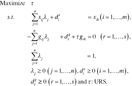
By duplicating Model (3.15) and adding an additional constraint of ![]() into the formulation, the radial model7, or input‐oriented RM(v), has the following mathematical structure to measure an efficiency score (θ) of the specific k‐th DMU:
into the formulation, the radial model7, or input‐oriented RM(v), has the following mathematical structure to measure an efficiency score (θ) of the specific k‐th DMU:
where the side constraint ![]() is additionally incorporated into Model (4.1). Thus, the surface of a production possibility set for Model (4.1) is shaped by a convex polyhedral cone under variable RTS. It is possible for us to drop the side constraint from Model (4.1), as formulated in Model (3.15). In such a case, a production possibility set is characterized by constant RTS. Thus, Model (4.1) becomes input‐oriented RM(c) where (c) indicates the status of constant RTS.
is additionally incorporated into Model (4.1). Thus, the surface of a production possibility set for Model (4.1) is shaped by a convex polyhedral cone under variable RTS. It is possible for us to drop the side constraint from Model (4.1), as formulated in Model (3.15). In such a case, a production possibility set is characterized by constant RTS. Thus, Model (4.1) becomes input‐oriented RM(c) where (c) indicates the status of constant RTS.
The term ![]() becomes zero or negative on the optimality of Model (4.1). The objective value consists of an efficiency score8 and a total sum of slacks, where the latter is used to adjust the level of efficiency, or OE. Here, it is important to note that, if the slack adjustment term represents a level of inefficiency, then the sign before the term should be negative in the objective function in order to maintain the efficiency range between zero and unity. In contrast, Model (4.9), along with Equation (4.10), indicates a desirable output‐oriented model for RM(v) that is used for measuring a level of inefficiency in the objective function. In the case, the sign becomes positive. See Chapter 17, as well.
becomes zero or negative on the optimality of Model (4.1). The objective value consists of an efficiency score8 and a total sum of slacks, where the latter is used to adjust the level of efficiency, or OE. Here, it is important to note that, if the slack adjustment term represents a level of inefficiency, then the sign before the term should be negative in the objective function in order to maintain the efficiency range between zero and unity. In contrast, Model (4.9), along with Equation (4.10), indicates a desirable output‐oriented model for RM(v) that is used for measuring a level of inefficiency in the objective function. In the case, the sign becomes positive. See Chapter 17, as well.
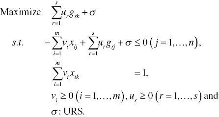
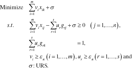
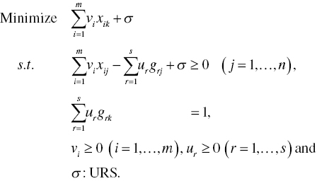
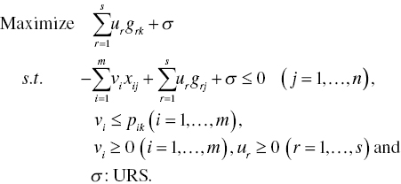
To describe the methodological strengths and drawbacks of Model (4.1), this chapter prepares the dual formulation of Model (4.1) that is mathematically specified as follows:
Here, V = (v1,…,vm) and U = (u1,…,us) are two row vectors of dual variables related to the first and second sets of constraints in Model (4.1). An unrestricted dual variable (σ) is derived from the third constraint of Model (4.1). In transforming from Model (4.1) to Model (4.2), this chapter implicitly treats that ![]() and
and ![]() are changed to
are changed to ![]() for all i and
for all i and ![]() for all r in Model (4.2).
for all r in Model (4.2).
It is important to note that the objective function of Model (4.1) equals that of Model (4.2) on optimality. Thus, the level of OE is determined by
on the optimality of Models (4.1) and (4.2).
A methodological benefit of Model (4.1) is that all dual variables (![]() for all i and
for all i and ![]() for all r) are strictly positive in their signs, so being able to function as multipliers on production factors. As a result, their information is fully utilized in performance evaluation although some dual variables may become very small as multipliers in such a manner that
for all r) are strictly positive in their signs, so being able to function as multipliers on production factors. As a result, their information is fully utilized in performance evaluation although some dual variables may become very small as multipliers in such a manner that ![]() for some i and
for some i and ![]() for some r. This analytical feature is very important in measuring a type of RTS, a marginal rate of transformation (MRT), a rate of substitution (RSU) between production factors and other scale related measures, all of which will be discussed in Chapters 8, 20 and 22.
for some r. This analytical feature is very important in measuring a type of RTS, a marginal rate of transformation (MRT), a rate of substitution (RSU) between production factors and other scale related measures, all of which will be discussed in Chapters 8, 20 and 22.
4.2.2 Underlying Concept
This book conveys a message that DEA can be used for the measurement of not only an efficiency score but also other important measures (e.g., RTS and other scale measures). Thus, DEA can be considered as a holistic approach for performance assessment. Consequently, it is necessary for us to satisfy various conditions on DEA solutions. One of such conditions, for example, is that all dual variables should be strictly positive. Of course, the requirement may drop in many decisional cases, depending upon the type of these applications. See Chapters 9, 21, 22 and 23 in which some dual variables are unrestricted in their signs.
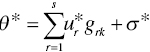
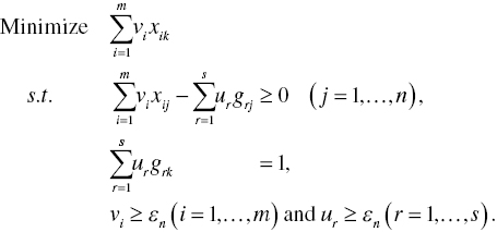
A drawback of Model (4.1) is that εn is a prescribed small number, often referred to as a non‐Archimedean small number. The specification9 of εn incorporates a subjective decision by a DEA user(s). In reality, none knows what the small number is. As a result, many users often drop the non‐Archimedean small number in their efficiency assessments. Model (4.1) without the very small number becomes
As mentioned previously, when we measure the level of OE concerning the k'th DMU, Models (4.1) and (4.4) may not produce any major difference between them because εn is the very small number. The elimination is seemingly acceptable. However, a serious problem may occur in the dual model whose multipliers, obtained from dual variables, may be zero. Such a result is unacceptable in this book on environmental assessment because it is impossible to measure RTS and the other type of scale measures (e.g., rate of substitution). See, for example, Chapters 22 and 23.
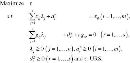
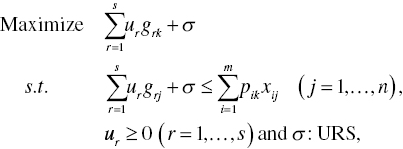
The dual formulation of Model (4.4) has the following structure:
Here, all mathematical descriptions in Model (4.2) are applicable to Model (4.5).
The objective value of Model (4.4) equals that of Model (4.5) on optimality. Thus, the level of OE is determined by
on the optimality of Models (4.4) and (4.5).
In addition to the above description, Models (4.4) and (4.5) have the other two important features. One of the two features is that Model (4.5) has ![]() because θ is unrestricted (URS) in Model (4.4). In other words, the upper bound of θ* is unity in Model (4.4), indicating the status of full efficiency, because the first constraints indicate
because θ is unrestricted (URS) in Model (4.4). In other words, the upper bound of θ* is unity in Model (4.4), indicating the status of full efficiency, because the first constraints indicate ![]() in Model (4.5) for the k‐th DMU. The left hand side of the equation is the objective value of Model (4.5). Hence, both Models (4.4) and (4.5) indicate
in Model (4.5) for the k‐th DMU. The left hand side of the equation is the objective value of Model (4.5). Hence, both Models (4.4) and (4.5) indicate ![]() on the optimality of the k‐th DMU. There is no lower bound on θ* because the efficiency score is expected to be unrestricted in Model (4.4). However, a conventional use of the efficiency score, applied to a cross‐sectional data set, becomes non‐negative10 because Model (4.5) is structured by a maximization problem within an efficiency frontier.
on the optimality of the k‐th DMU. There is no lower bound on θ* because the efficiency score is expected to be unrestricted in Model (4.4). However, a conventional use of the efficiency score, applied to a cross‐sectional data set, becomes non‐negative10 because Model (4.5) is structured by a maximization problem within an efficiency frontier.
The other concern is that ![]() (i = 1,…, m) and
(i = 1,…, m) and ![]() (r = 1,…, s) in Model (4.5) may have a possible occurrence of
(r = 1,…, s) in Model (4.5) may have a possible occurrence of ![]() for some i and/or
for some i and/or ![]() for some r. This clearly indicates that some production factors are not utilized in the efficiency assessment, so being problematic as mentioned previously. Therefore, the original DEA study (i.e., Charnes et al., 1978) incorporates
for some r. This clearly indicates that some production factors are not utilized in the efficiency assessment, so being problematic as mentioned previously. Therefore, the original DEA study (i.e., Charnes et al., 1978) incorporates ![]() into the objective function of Model (4.1). As a result of such incorporation, Model (4.2) has
into the objective function of Model (4.1). As a result of such incorporation, Model (4.2) has ![]() (i = 1,…, m) and
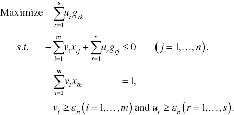
(i = 1,…, m) and ![]() (r = 1,…, s) so that all dual variables, or multipliers, are strictly positive in their signs. However, as mentioned previously, a problem of the non‐Archimedean small number (εn) is that none knows what it is in reality. Consequently, a subjective decision is included in the selection process of εn. Chapter 7 discusses how to handle the difficulty by incorporating strong complementary slackness conditions (SCSCs) into Models (4.4) and (4.5). The approach can overcome the difficulty related to εn so that it can avoid our selection subjectivity.
(r = 1,…, s) so that all dual variables, or multipliers, are strictly positive in their signs. However, as mentioned previously, a problem of the non‐Archimedean small number (εn) is that none knows what it is in reality. Consequently, a subjective decision is included in the selection process of εn. Chapter 7 discusses how to handle the difficulty by incorporating strong complementary slackness conditions (SCSCs) into Models (4.4) and (4.5). The approach can overcome the difficulty related to εn so that it can avoid our selection subjectivity.
4.2.3 Input‐Oriented RM(c) under Constant RTS
Models (4.1) and (4.2) are formulated under variable RTS. If Model (4.1) drops ![]() , then the dual variable (σ) becomes zero in Model (4.2). In the case, the primal and dual models imply the status of constant RTS on their production possibility sets. The input‐oriented RM(c) under constant RTS has the following primal and dual formulations:
, then the dual variable (σ) becomes zero in Model (4.2). In the case, the primal and dual models imply the status of constant RTS on their production possibility sets. The input‐oriented RM(c) under constant RTS has the following primal and dual formulations:
and:
Here, all mathematical descriptions on dual variables in Model (4.2) are applicable to Model (4.8).
As mentioned previously, it is possible to drop ![]() in the objective function of Model (4.7) as found in many research efforts on production economics. In the case, it is necessary for us to examine whether all dual variables are positive or not on the optimality of Model (4.8). The objective value of Model (4.7) equals that of Model (4.8) on optimality.
in the objective function of Model (4.7) as found in many research efforts on production economics. In the case, it is necessary for us to examine whether all dual variables are positive or not on the optimality of Model (4.8). The objective value of Model (4.7) equals that of Model (4.8) on optimality.
4.3 RADIAL MODELS: DESIRABLE OUTPUT‐ORIENTED
4.3.1 Desirable Output‐oriented RM(v) under Variable RTS
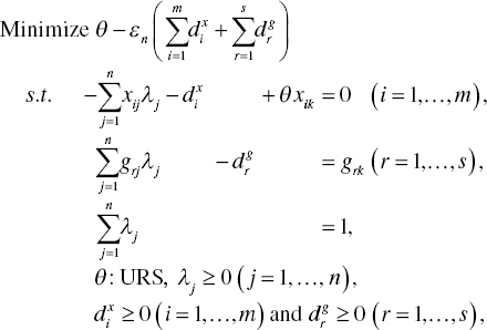
As a methodological alternative of the input‐oriented RM(v) and RM(c), previous DEA studies have paid attention to the following desirable output‐oriented model, or RM(v), to estimate an efficiency score (θ) regarding the k‐th DMU:
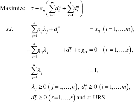
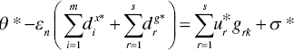
The level of OE (θ*) is measured by an unrestricted measure (τ *) and slacks on the optimality of Model (4.9) as follows:
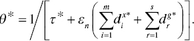
There are two important concerns associated with Model (4.9). One of these concerns is that the objective value of Model (4.9) becomes more than unity (![]() ) on optimality. Therefore, the OE measure of desirable output‐oriented RM(v) is determined by Equation (4.10). The other concern is that the objective function of Model (4.9) incorporates a positive sign before the term regarding the total sum of slacks like
) on optimality. Therefore, the OE measure of desirable output‐oriented RM(v) is determined by Equation (4.10). The other concern is that the objective function of Model (4.9) incorporates a positive sign before the term regarding the total sum of slacks like ![]() , not
, not ![]() as found in Model (4.7), because τ* does not directly indicate the level of OE. Rather, the level of OE (θ*) is measured by the reciprocal of the inefficiency score via Equation (4.10).
as found in Model (4.7), because τ* does not directly indicate the level of OE. Rather, the level of OE (θ*) is measured by the reciprocal of the inefficiency score via Equation (4.10).
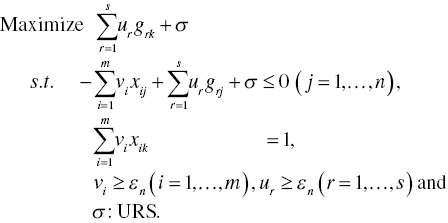
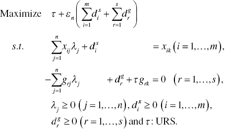
Model (4.9) has the following dual formulation:
Here, all mathematical descriptions on dual variables in Model (4.2) are applicable to Model (4.11) by changing inputs to desirable outputs.
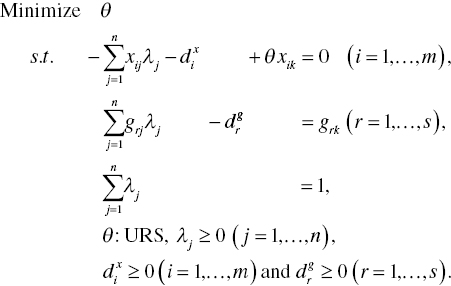
As mentioned previously, it is possible to drop the non‐Archimedean small number (εn) from Model (4.9) and Equation (4.10). In such a case, the desirable output‐oriented RM(v) becomes
The level of OE (θ*) is measured by an unrestricted measure (τ *) by
Model (4.12) has the following dual formulation:
Here, all the descriptions for the input‐oriented RM(v) in Model (4.5) are applicable to Model (4.14).
4.3.2 Desirable Output‐oriented RM(c) under Constant RTS
It is possible to reorganize Model (4.9) under constant RTS that measures the level of OE (θ *) as follows:
Model (4.15) drops ![]() from Model (4.9). The OE (θ*) is measured by an unrestricted measure (τ*) via
from Model (4.9). The OE (θ*) is measured by an unrestricted measure (τ*) via ![]() . The elimination of the side constraint makes it possible to measure the desirable output‐oriented RM(c) under constant RTS.
. The elimination of the side constraint makes it possible to measure the desirable output‐oriented RM(c) under constant RTS.
The dual formulation of Model (4.15) has the following formulation:
Here, ![]() and
and ![]() are two row vectors of dual variables related to the first and second sets of constraints in Model (4.15).
are two row vectors of dual variables related to the first and second sets of constraints in Model (4.15).
As an extension of Models (4.15) and (4.16), this chapter reorganizes them as follows:
The efficiency score (θ*) is measured by an unrestricted measure (τ*) via ![]() .
.
The dual formulation of Model (4.17) has the following formulation:
See a description of Model (4.16) regarding ![]() and
and ![]() .
.
4.4 COMPARISON BETWEEN RADIAL MODELS
4.4.1 Comparison between Input‐Oriented and Desirable Output'Oriented Radial Models
There are several differences between the four radial models (RMs), two of which are summarized as follows. One of the two differences is that an efficiency score of the input‐oriented RM(v) is different from that of the desirable output‐oriented RM(v) under variable RTS. In contrast, the efficiency measure of input‐oriented RM(c) equals that of desirable output‐oriented RM(c) under constant RTS. See Proposition 4.1 about the mathematical proof. The other difference is shown in Figure 4.1 which depicts a visual difference between efficiency frontiers under constant RTS and variable RTS in the x–g domain. A straight line from the origin indicates an efficiency frontier under constant RTS, while a piece‐wise linear contour line, or {A‐B‐C‐D}, indicates the efficiency frontier under variable RTS.
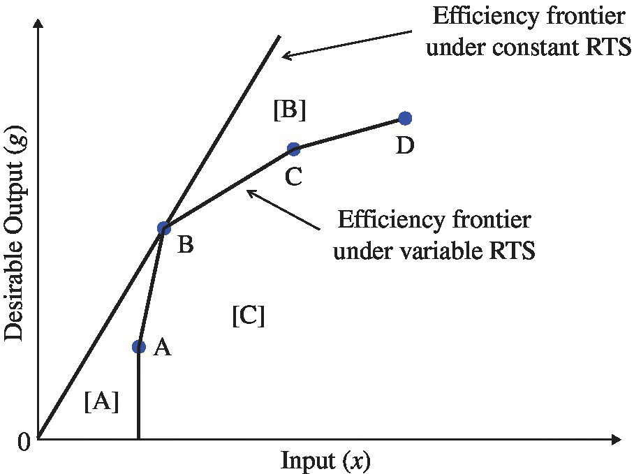
FIGURE 4.1 Efficiency frontiers under constant and variable RTS
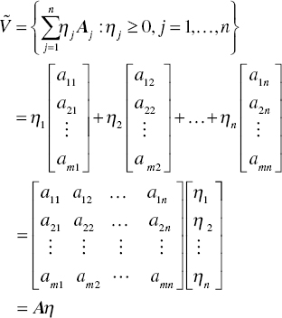
As depicted in Figure 4.1, the two production possibility sets imply two areas for covering a possible combination between inputs and desirable outputs. They are axiomatically specified as follows:
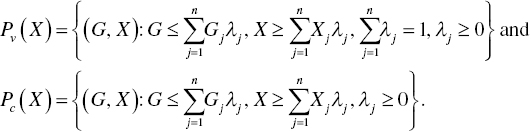
The first production possibility set is formulated under variable RTS, or “VRTS,” while the second one is formulated by constant RTS, or “CRTS” in Equation (4.19). The difference between the two production possibility sets can be found in only the incorporation of ![]() . In Figure 4.1, the first production possibility set under variable RTS consists of the area [C] and the second one under constant RTS consists of the three areas expressed by [A]∪[B]∪[C] where the symbol ∪ indicates a union set.
. In Figure 4.1, the first production possibility set under variable RTS consists of the area [C] and the second one under constant RTS consists of the three areas expressed by [A]∪[B]∪[C] where the symbol ∪ indicates a union set.
In examining RM(c), it is necessary for this chapter to prove the following proposition:
4.4.2 Hybrid Radial Model: Modification
As an extension of the radial models, we can control the sum of structural (intensity) variables by adding the lower (lb) and upper (ub) bounds, or ![]() in the proposed RM formulations. Such models are often referred to as “hybrid models” in the DEA community.
in the proposed RM formulations. Such models are often referred to as “hybrid models” in the DEA community.
To discuss a hybrid model, this chapter considers it by adding the condition on the lower and upper bounds in Model (4.1). The hybrid model for input‐oriented measurement becomes
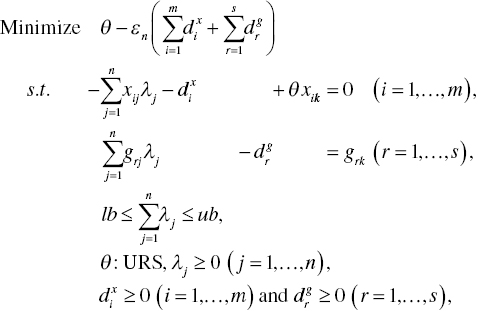
where the previous side constraint ![]() for variable RTS in Model (4.1) is replaced by the new one
for variable RTS in Model (4.1) is replaced by the new one ![]() in Model (4.23).
in Model (4.23).
The dual formulation of Model (4.23) becomes as follows:
Using Model (4.23), the input‐oriented radial measurement is classified into the following three categories, for example: (a) ![]() (b)
(b) ![]() , and (c)
, and (c) ![]() under increasing RTS, respectively. This type of classification can be applied to the desirable output‐oriented radial model, as well. See Tone (1993) for the first discussion on the hybrid expression on RM. See also Sueyoshi (1997) which provided a detailed description on the hybrid expression and its applications.
under increasing RTS, respectively. This type of classification can be applied to the desirable output‐oriented radial model, as well. See Tone (1993) for the first discussion on the hybrid expression on RM. See also Sueyoshi (1997) which provided a detailed description on the hybrid expression and its applications.
4.5 MULTIPLIER RESTRICTION AND CROSS‐REFERENCE APPROACHES
An empirical difficulty of the proposed radial models is that they often suffer from an occurrence of many efficient DMUs. For example, among 100 DMUs, 90 DMUs are efficient and the remaining 10 DMUs are inefficient. Such an occurrence is mathematically acceptable but managerially unacceptable, because it is difficult for us to determine the rank of efficient DMUs. It is important to note that the type of problem often occurs on all types of DEA models.
4.5.1 Multiplier Restriction Methods
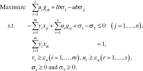
Assurance Region (AR) Analysis: To reduce the number of efficient DMUs by restricting the range of multipliers (i.e., dual variables), Thompson et al. (1986), Dyson and Thanassoulis (1988) and others proposed the use of AR analysis, which was discussed at the initial stage of DEA development. AR analysis incorporates the following multiplier restrictions into the dual formulations of the proposed RMs:
where the ratio of the i‐th input multiplier to the first one is expressed by its lower and upper bounds. The ratio combinations are applicable to the r‐th desirable output to the first one, as specified in Equation (4.25). It is trivial that multipliers are usually reqiured to be positive in many cases, whose magnitudes are expected to be much larger than εn.
Equation (4.25) is further extendable by the following input and desirable output weighted measure on the specific k‐th DMU:
where the ratio is determined by the i‐th weighted input divided by the sum of the total weighted inputs. In a similar manner, the ratio can be applied to the r‐th desirable output as formulated in Equation (4.26). Each equation indicates the importantce of the i‐th input and the r‐th desirable output among these production factors.
Figure 4.2 visually describes an implication of multiplier restriction in the data domain of two inputs (x1 and x2). All DMUs from {D1} to {D5}, consisting of an efficiency frontier, have the same magnitude of a desirable output so that the figure drops it. Let us consider A1 and A2 as the two vectors to restrict input multipliers. They are used as the upper and lower bounds for the multiplier restriction, expressed by Ṽ in Figure 4.2.
FIGURE 4.2 Multiplier restriction (a) The figure is prepared for our visual convenience. The number of efficient DMUs decreases from five {D1‐D2‐D3‐D4‐D5} on the efficiency frontier to one, {D3}. It is necessary for us to understand that strong multiplier restriction often produces an infeasible solution on optimality. The two directional vectors (A1 and A2) are used to restrict the direction of input multipliers. (b) It is assumed that all DMUs produce the same amount of a desirable output.
As a result of such multiplier restriction, the number of efficient DMUs decreases from five to one, that is, {D3} because only the DMU can exist only within the multiplier range (Ṽ) for inputs. This chapter uses Ṽ because input multipliers are applied for restriction on vi (i = 1,…, m).
The proposed AR analysis has two difficulties in the practical uses. One of the two difficulities is that the approach depends upon prior information (e.g., expreience and previous emprical evidence) for multiplier restriction. It is often difficult for us to assess such prior information. The other difficulty is that the approach may produce an infeasible solution on optimality as a result of strict restriction. It is necessary for us to carefully think how to restrict multipliers on a use of the AR approach. This type of difficulty will be solved in DEA environmental assessment. See Chapters 22 and 23 which describe a new type of multiplier restriction, referred to as “explorative analysis,” which does not use any prior information along with a data adjustment. The AR analisis does not incoporate the data adjustment.
4.5.2 Cone Ratio Method
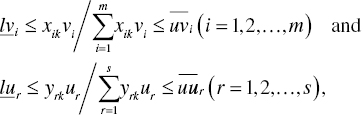
As mentioned previously, DEA produces many efficient DMUs. Charnes et al. (1989) and Brockett et al. (1997) proposed another type of approach for multiplier restriction, referred to as the “cone ratio (CR) method,” to reduce the number of efficient DMUs. To describe the methodology, this chapter starts from the following non‐negative input vector with m components, where the vector and matrix notations are for our visual convenience:
where ![]() is used for a column vector for input restriction (j = 1,…, n). The symbol (Tr) stands for a vector or matrix transpose. The restriction vector Ṽ is a (1 × m) column vector. So, ṼTr becomes a (m × 1) row vector.
is used for a column vector for input restriction (j = 1,…, n). The symbol (Tr) stands for a vector or matrix transpose. The restriction vector Ṽ is a (1 × m) column vector. So, ṼTr becomes a (m × 1) row vector.
In a similar manner, this chapter specifies the non‐negative directional vector for desirable outputs with s components as follows:
where ![]() is used for a column vector for restriction on desirable outputs (j = 1,…, n). The restriction vector Ũ is a (1 × s) column vector. So, ŨTr becomes a (s × 1) row vector.
is used for a column vector for restriction on desirable outputs (j = 1,…, n). The restriction vector Ũ is a (1 × s) column vector. So, ŨTr becomes a (s × 1) row vector.
Using Equations (4.27) and (4.28), the input‐oriented RM(c), or Model (4.8), becomes the following vector notation under the proposed CR method:
where ![]() is a raw vector of s dual variables for desirable outputs,
is a raw vector of s dual variables for desirable outputs, ![]() is a raw vector of m dual variables for inputs,
is a raw vector of m dual variables for inputs, ![]() is a column vector of m observed inputs of the j‐th DMU,
is a column vector of m observed inputs of the j‐th DMU, ![]() is a column vector of m observed inputs of the specific k‐th DMU and
is a column vector of m observed inputs of the specific k‐th DMU and ![]() is a column vector of s observed desirable outputs of the j‐th DMU.
is a column vector of s observed desirable outputs of the j‐th DMU.
Model (4.29) can be reorganized by incorporating Equations (4.27) and (4.28). The resulting formulation becomes
Here, ![]() in Model (4.29) are replaced by
in Model (4.29) are replaced by ![]() and
and ![]() in Model (4.30).
in Model (4.30).
The dual formulation of Model (4.30) becomes as follows:
Like the AR analysis, the proposed CR method has also a difficulty in both accessing prior information and being often infeasible on optimality. Another difficulty of the CR method is that the AR analysis is more intutive and easily used than the CR method. Therefore, Chapters 22 and 23 extend the AR analysis, not the CR method, to prepare “explorative analysis.” A benefit of CR is that it requires less computation time than AR because CR has less constraints than AR in the formulation. See Chapter 10 on DEA network computing which takes advantage of the mathematical structure with less constraints in the formulation.
4.5.3 Cross‐reference Method
Besides the multilier restriction approaches, a cross‐reference method is widely used by many DEA researchers to classify efficient DMUs into two categories. One of the two categories includes efficient ones that locate on a vertex of an efficiency frontier. The other category includes the other efficient ones that locate on the efficiency frontier, but not locating on the vertex. See the DMU classification discussed in Chapter 9 (for algorithm development for network computing). Also, see Charnes et al. (1986, 1991) for the original DMU classification, parts of which are used in this chapter. A gist of the cross‐reference method is the classification of DMUs on an efficiency frontier.
In this chapter, the three groups of DMUs are characterized by an optimal solution of radial measurement regrading the k‐th DMU, for example, by Model (4.20) with slacks. The assumption on constant RTS is necessary so that the proposed cross‐reference method, using RM(c), can produce a feasible solution on optimality. In contrast, RM(v) may produce an infeasible solution in the case of variable RTS.
The three groups of DMU classifications considered in this chapter are mathematically specfied in the following manner:
Here, all DMUs are expressed by a whole set (J).
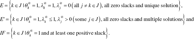
The first two groups of efficient DMUs locate on an efficiency frontier. The efficient group of DMUs (E) locates on the vertexes of an efficiency frontier. The efficient DMUs in the other group (E′) locate between such efficient DMUs that belong to E. The DMUs in E′ may suffer from an occurrence of multiple solutions on a combination(s) of a reference set. The last group (IF) consists of inefficient DMUs, but they exist on the efficiency frontier. They are not efficient because of at least one positive slack.
As mentioned previously, DEA may produce many efficient DMUs in ![]() . Therefore, it is necessary for us to classify them further if we want to prepare their ranking assessment. That is the purpose of the cross‐reference method. See Chapter 25 on the ranking analysis.
. Therefore, it is necessary for us to classify them further if we want to prepare their ranking assessment. That is the purpose of the cross‐reference method. See Chapter 25 on the ranking analysis.
To describe the proposed approach, let us select DMU {a}, belonging to ![]() and return to input‐based RM(c), or Model (4.20), to obtain the computational feasibility. The cross‐reference efficiency
and return to input‐based RM(c), or Model (4.20), to obtain the computational feasibility. The cross‐reference efficiency ![]() of the b‐th DMU in J is measured by the following radial model (e.g., Doyle and Green, 1994; Green et al., 1996):
of the b‐th DMU in J is measured by the following radial model (e.g., Doyle and Green, 1994; Green et al., 1996):
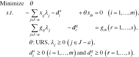
An important feature of Model (4.33) is that if the efficient DMU {a} belongs to E, then the elimination changes the shape of an efficiency frontier. As a result, the degree of ![]() may be changed from the original efficiency measure. In contrast, if it belongs to E′, then the elimination does not make any change on the frontier shape because it does not locate on the vertex of an efficiency frontier. In the case, the degree of
may be changed from the original efficiency measure. In contrast, if it belongs to E′, then the elimination does not make any change on the frontier shape because it does not locate on the vertex of an efficiency frontier. In the case, the degree of ![]() does not produce any efficiency change. Thus, the cross‐reference method can provide us with a new measure on efficient DMUs, based upon which we can classify them. The most important benefit of the proposed approach is that it is possible for us to measure a degree of cross‐reference of the a‐th DMU in
does not produce any efficiency change. Thus, the cross‐reference method can provide us with a new measure on efficient DMUs, based upon which we can classify them. The most important benefit of the proposed approach is that it is possible for us to measure a degree of cross‐reference of the a‐th DMU in ![]() by examining the degree of
by examining the degree of ![]() . In this case,
. In this case, ![]() may be more than unity so that
may be more than unity so that ![]() becomes positive. Thus, all efficient DMUs in group E on the vertexes of an efficiency frontier are reevaluated by the degree of
becomes positive. Thus, all efficient DMUs in group E on the vertexes of an efficiency frontier are reevaluated by the degree of ![]() . Thus, the cross‐reference method can provide us with an additional measure on efficient DMUs, based upon which we can classify them for ranking analysis.
. Thus, the cross‐reference method can provide us with an additional measure on efficient DMUs, based upon which we can classify them for ranking analysis.
Finally, it is important to note three concerns on a use of the cross‐reference method. First, the approach is feasible under constant RTS, but it may produce an infeasible solution under variable RTS. Second, there is no theoretical rationale on the validity of the cross‐reference method although it intuitively appeals to DEA users. Finally, the assessment on efficient DMUs is based upon local evaluation by considering a limited number of efficient DMUs in a reference set. It does not cover the group‐wide performance assessment of all DMUs by using a single set of common multipliers (weights) on efficient DMUs. See, for example, Chapter 25 that discusses how to determine common multipliers for the group‐wide assessment. Thus, the cross‐reference approach has a high level of computational tractability on DMU ranking analysis, but lacking any theoretical support within the framework of RM(c).
4.6 COST ANALYSIS
4.6.1 Cost Efficiency Measures
A methodological benefit of the radial measurement is that it can conceptually connect these models to cost efficiency analysis that minimizes the amount of total production cost (Sueyoshi, 1999b). Assuming that we can access an input price vector, or ![]() , of all DMUs (j = 1,…, n), the cost efficiency of the k‐th DMU is measured by the following model:
, of all DMUs (j = 1,…, n), the cost efficiency of the k‐th DMU is measured by the following model:
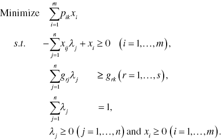
Here, ![]() is an unknown input quantity vector, not an observed vector as previously discussed for radial models, or RMs. It is important to note that Model (4.34) does not incorporate slacks into the formulation because it looks for an input vector that attains cost minimum, not an efficiency score. Moreover, dual variables become positive, as discussed below, because an input‐related dual vector corresponds to an input price vector. Therefore, this chapter needs to drop a slack vector in the objective function of Model (4.34).
is an unknown input quantity vector, not an observed vector as previously discussed for radial models, or RMs. It is important to note that Model (4.34) does not incorporate slacks into the formulation because it looks for an input vector that attains cost minimum, not an efficiency score. Moreover, dual variables become positive, as discussed below, because an input‐related dual vector corresponds to an input price vector. Therefore, this chapter needs to drop a slack vector in the objective function of Model (4.34).
The cost efficiency of the k‐th DMU is determined by the following manner (Farrell, 1957):
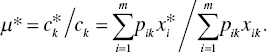
The cost efficiency implies the mimimized cost divided by an observed cost regrading the k‐th DMU.
The dual formulation of Model (4.34) becomes:
On optimality, both primal and dual models have a cost minimum expressed by ![]() . Moreover,
. Moreover, ![]() always exsist between the two models as part of complementary slackness conditions (CSCs) of linear programming. If
always exsist between the two models as part of complementary slackness conditions (CSCs) of linear programming. If ![]() for all i, then Model (4.36) becomes the following condensed formulation:
for all i, then Model (4.36) becomes the following condensed formulation:
because ![]() is maintained on the optimality of Model (4.37). Equation (4.35) indicates that the cost minimum of the k‐th DMU is less than or equal all the cost estimates measured by its observed input price vector.
is maintained on the optimality of Model (4.37). Equation (4.35) indicates that the cost minimum of the k‐th DMU is less than or equal all the cost estimates measured by its observed input price vector.
4.6.2 Type of Efficiency Measures in Production and Cost Analyses
Previous discussions used the term “efficiency.” Hereafter, the concept of efficiency is separated into more specific classifications related to the proposed input‐oriented radial measurement. Some of these efficiency meaures were first conceptually specified by Farrell (1957) in the case of a single desirable output with multiple inputs under constant and diminishing RTS. Then, Sueyoshi (1999b) elaborated them by extending these production factors under constant RTS and variable RTS.
The efficiency measures used in this chapter are specified as follows:
- Operational efficiency (OEv) under variable RTS: the degree of opetational efficincy that is measured by the optimal objective value of RM(v), for example, Model (4.1),
- Operational and Scale Efficiency (OEc) under constant RTS: the degree of operational efficiency that is measured by the optimal objective value of RM(c), for example, Model (4.7),
- Production‐based scale efficiency (PSE):
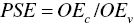 .
. - Cost efficiency (CEv) under variable RTS:
 from Equation (4.35) via Model (4.34),
 - Cost and Scale Efficiency (CEc) under constant RTS:
 from Equation (4.35) via Model (4.34) without
  .
. - Cost‐based scale efficiency (CSE):
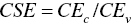 .
. - Allocative efficiency (AEv) under variable RTS:
 .
. - Allocative and scale efficiency (AEc) under constant RTS:
The desirable output‐oriented measures have another type of efficiency classifications. This chapter discribes only the input‐oriented efficiency ones because they can directly link to cost‐based efficiency concepts.
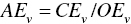
Figure 4.3 visually describes various efficiency measures, all of which are defined by the eight classifications: (a–h) as discussed above. The figure has two efficiency frontiers, depending upon the assumption on RTS (i.e., constant or variable). The efficiency frontier, consisting of a piece‐wise linear contour line, or DMUs {F‐G‐B‐H‐I‐J}, is shaped under variable RTS, while the other curve (I–I′) is shaped under constant RTS. For our descriptive convenience in Figure 4.3, this chapter starts with a visual explanation on OEV.
FIGURE 4.3 Efficiency measures (a).
Source: Sueyoshi, (1997)
The degree of OEV is visually specified by the distance OB/OA under variable RTS, where OB stands for a distance between the origin O and DMU {B}. In a simular manner, OA indicates the distance between the origin O and DMU {A}. This chapter drops the term DMU if a specified point in the figure is used to indicate a projected point, so not indicating a DMU. Shifting from variable to constant RTS, OEc is measured by OC/OA. The difference between the two measures is expressed by PSE = OEc/OEv = (OC/OA)/(OB/OA) = OC/OB. For example, DMU {A} needs to reduce the amount of an input vector from {A} to {B} under variable RTS. The level of such input reduction, indicating an amount of inefficiency, is expressed by the distance of (OA–OB)/OA. By controling the operation size, the DMU {A} can attain the input decrease until it attains a projected point, C. The inefficiency due to an inapproporiate operation size is expressed by (OB–OC)/OA. Thus, OEC is separated into two components in the manner of ![]() .
.
The production‐based description can be applied to the cost‐based one such as CEv, CEc and CSE. Given an input price vector (P), H indicates the cost‐minimum for DMU {A} in the case of variable RTS. Here, lines p1–p1′ and p2–p2′ indicate a level of cost under a fixed ratio of input prices with p1/p2. D and H locate on the line (p2 and p2′), with both having the same value of cost‐minimum. Therefore, CEv = OD/OA. If the line is closer to the origin, the level of cost is lower. Meanwhile, under constant RTS, K indicates such a cost‐minimum. The total production cost becomes same on K and E because both points locate on the line (p1 and p1′). Therefore, CEc= OE/OA. The degree of CSE is determined by the ratio between CEv and CEc. Thus, this chapter has CSE = CEc/CEv = (OE/OA)/(OD/OA) = OE/OD. The decomposition related to the cost minimization process indicates that DMU {A} needs to attain H by an effort for cost mimimization and further attain K by controlling its operational size.
In addtion to these efficiency concepts, AEv and AEc have unique features that cannot be found in the other efficiency measures. For example, the degree of AEv is determined by ![]() and AEV = (OD/OA)/(OB/OA) = OD/OB in Figure 4.3. Given an input price vector (P), the efficiency measure indicates how each DMU controls the ratio of input allocation by itself for cost‐mimimization under variable RTS. The degree of AEC has the same implication under constant RTS.
and AEV = (OD/OA)/(OB/OA) = OD/OB in Figure 4.3. Given an input price vector (P), the efficiency measure indicates how each DMU controls the ratio of input allocation by itself for cost‐mimimization under variable RTS. The degree of AEC has the same implication under constant RTS.
4.6.3 Illustrative Example
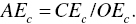
Table 4.1 lists a data set to discuss three efficiency measures related to two radial models. The table contains eight DMUs {A–H}, each of which uses one input to produce one desiable output. Table 4.2 summarizes computational results on OEv, OEc and PSE. Figure 4.4 visually describes OEv measures under variable RTS and OEc measures under constant RTS, both are associated with the two efficiency frontiers.
TABLE 4.1 An illustrative example
| DMU | A | B | C | D | E | F | G | H |
| Input | 2 | 3 | 7 | 10 | 5 | 7 | 8 | 10 |
| Desirable Output | 1 | 4 | 7 | 8 | 3 | 6 | 2 | 4 |
TABLE 4.2 Production‐based efficiency measures
| DMU | A | B | C | D | E | F | G | H |
| OEv | 1 | 1 | 1 | 1 | 0.533 | 0.810 | 0.292 | 0.300 |
| OEc | 0.375 | 1 | 0.750 | 0.600 | 0.450 | 0.643 | 0.188 | 0.300 |
| PSE | 0.375 | 1 | 0.750 | 0.600 | 0.844 | 0.794 | 0.643 | 1 |
FIGURE 4.4 Input‐oriented projections and two efficiency frontiers
The formulation to measure OEV of DMU {A}, for example, is formulated as follows:
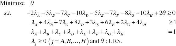
It is necessary to repeat the computation process on DMU {A} to measure the other DMUs {B–H}.
As listed in Table 4.2, along with Figure 4.4, only DMU {B} attains the status of efficiency in the three measures. The four DMUs {A, B, C and D} attain the status of efficiency on OEv under variable RTS, but only DMU {B} become efficient under constant RTS. The other DMUs {E, F, G and H} have exhibited some level of inefficiency on OEv. To describe the implication of PSE, measured by OEc/OEv, let us pay attention to the inefficient DMU {F}. Since the computational results of Table 4.2 are determined by the input‐oriented measurement, the ideal performance of DMU {F} can be found in a projected point R on the efficiency frontier under variable RTS and another projected point Q under constant RTS.
The degree of OEv on DMU {F} is measured by PR/PF = 0.810. The degree of OEc is measured by PQ/PF = 0.643. Based upon the two efficiency measures, the degree of PSE on the DMU is determined by OEc/OEv = (PQ/PF)/(PR/PF) = PQ/PR = 0.643/0.810 = 0.794. The description of DMU {F} in terms of the three efficiency measures is applicable regarding the other DMUs.
Table 4.3 lists a data set to discuss eight efficiency measures related to production and cost‐based efficiency measures. First, let us describe the formulation to measure the level of CEv on DMU {F}, for example, which is structured as follows:
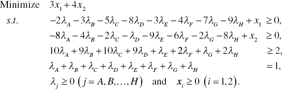
TABLE 4.3 An illustrative example
| DMU | A | B | C | D | E | F | G | H |
| Input 1 | 2 | 3 | 5 | 8 | 3 | 4 | 7 | 9 |
| Input 2 | 8 | 4 | 2 | 1 | 9 | 6 | 2 | 8 |
| Desirable Output | 10 | 9 | 10 | 9 | 1 | 2 | 1 | 2 |
| Price of Input 1 | 3 | 4 | 2 | 1 | 2 | 3 | 3 | 4 |
| Price of Input 2 | 3 | 1 | 3 | 2 | 2 | 4 | 1 | 2 |
Table 4.4 summarizes eight efficiency measures related to production and cost analyses. As summarized in the table, DMU {C} is efficient in terms of the eight measures. The DMUs {A, B, D} have mixed efficiency measures in the eight measures and the remaining DMUs {E, F, G, H} are inefficient in these measures.
TABLE 4.4 Production and cost‐based efficiency measures
| DMU | A | B | C | D | E | F | G | H |
| OEv | 1 | 1 | 1 | 1 | 0.762 | 0.727 | 0.846 | 0.412 |
| OEc | 1 | 1 | 1 | 1 | 0.078 | 0.160 | 0.087 | 0.088 |
| PSE | 1 | 1 | 1 | 1 | 0.103 | 0.220 | 0.103 | 0.214 |
| CEv | 0.700 | 1 | 1 | 0.900 | 0.583 | 0.639 | 0.565 | 0.385 |
| CEc | 0.700 | 0.900 | 1 | 0.810 | 0.058 | 0.128 | 0.061 | 0.085 |
| CSE | 1 | 0.900 | 1 | 0.900 | 0.100 | 0.200 | 0.108 | 0.222 |
| AEv | 0.700 | 1 | 1 | 0.900 | 0.766 | 0.878 | 0.668 | 0.934 |
| AEc | 0.700 | 0.900 | 1 | 0.810 | 0.744 | 0.799 | 0.697 | 0.971 |
4.7 SUMMARY
This chapter discussed radial models that were widely used for the measurement of OEv and other seven efficiency measures (so, becoming a total of eight measures), all of which were obtained from the production and cost‐based measurements. The production‐based measurement is usually classified into radial measures under variable and constant RTS. This chapter extended production‐based radial measures into cost‐based measurement. As a result, this chapter provided an analytical linkage among these production and cost‐based models from their efficiency measures.
This chapter also described multiplier restriction methods (i.e., AR and CR) that specified the range of dual variables (multipliers). As a result, the proposed methods were expected to produce positive dual variables in the manner that they could reduce the number of efficient DMUs. It is widely known that DEA may produce many efficient DMUs. It is mathematically acceptable but managerially unacceptable because we cannot rank efficient DMUs. However, the multiplier restriction approaches (e.g., AR and CR) discussed in this chapter do not have any mathematical justification that they can always have positive dual variables. In the worst case, they produce an infeasible solution because of too strict restriction. To avoid such a difficulty, Chapter 7 proposes the incorporation of strong complementary slackness conditions (SCSCs) into DEA to obtain positive dual variables on efficient DMUs. It is not necessary to apply SCSCs to inefficient DMUs because they do not influence the degree of efficiency on all DMUs. Note that the use of SCSCs is not perfect in terms of ranking all DMUs. See Chapter 25 that extends a mathematical description on SCSCs for the ranking analysis.
In addition to the multiplier restriction methods, this chapter discussed the cross‐reference approach, which was useful in classifying efficient DMUs. A problem of the approach was that it reevaluated an efficient DMU based upon local comparison on part of DMUs on an efficient frontier, so not having any common weights or group‐wide evaluation including all DMUs (at least all efficient DMUs). Furthermore, there was no mathematical justification for the cross‐reference approach. Such were the drawbacks of the cross‐reference approach. See Chapter 25 that discusses how to obtain common weights for group‐wide evaluation.
At the end of this chapter, it is necessary for us to describe that there is no perfect DEA approach. Any approach has its methodological strength and weakness. Consequently, it is necessary for us to utilize DEA carefully by understanding such unique features. This concern will be extended to Chapter 6 that discusses a methodological bias issue, implying “different approaches produce different results,” on several DEA (radial and non‐radial) models.