6
Producing Fluorescent Nanodiamonds
Natural diamonds in colors are commonly known as fancies, or fancy color diamonds, in gemstone industries. They are rare, beautiful, and some even carry impressive price tags in the jewelry market. By comparison, micro‐ and nanoscale diamond powders are low in price, with or without colors and fluorescent or not. These powders have been used as abrasives for grinding and polishing purposes since ancient time, mainly because of their extraordinary hardness. Little or no attention has been paid over the centuries to other properties of nanodiamonds such as their innate biocompatibility and light‐emitting capability. The invention of fluorescent nanodiamond (FND) in 2005 has revolutionized the field, opening a new area of research and development with diamonds [1]. Experiments with FNDs in the last decade have demonstrated various promising applications of surface‐functionalized FNDs in diversified fields, ranging from physics and chemistry to biology and medicine [2]. It is worthy of noting that as originated from the discovery of Radium by Marie Skłodowska Curie (Section 3.2), FNDs may very well be called Madame Curie’s gemstones, valued appropriately as a scientist’s best friend.
In this chapter, we focus our attention on the principles and practices of producing FNDs in a large‐scale quantity, which is the first step towards broad applications of the nanomaterials in biology and nanoscale medicine (cf., Chapters 7–10). Additionally, we will explore the topics such as size reduction and spectroscopic characterization of FNDs at the ensemble level with various optical methods. Single particle detection is the subject of the next chapter.
As a reminder, the reader may wish to review some key concepts before proceeding to the details of the discussion in this chapter. These concepts include: (i) general characteristics of nanodiamonds (Section 2.2) and nitrogen impurities (Section 3.1), (ii) important spectral features of diamond color centers (Table 3.2), (iii) optical properties of NV0, NV−, and H3 (Section 3.3), and (iv) optically detected magnetic resonance (Section 3.4), which is one of the major players in the next few chapters.
6.1 Production
6.1.1 Theoretical Simulations
FNDs are diamond nanoparticles containing vacancy‐related color centers as fluorophores. Particles containing H3 centers are called green FNDs and particles containing NV centers are called red FNDs, corresponding to their emission colors. Structural defects like vacancies always exist in the crystal matrices of both natural and synthetic diamonds, although the concentration is low (typically <1 ppm). Studies on thermally annealed HPHT‐NDs have shown that the smallest nanodiamond particle able to host a stable NV center is approximately 8 nm in diameter [3]. This number corresponds to a NV concentration of 20 ppm, given that 1 ppm is equal to 1.76 × 10¹⁷ atoms cm−3 in diamond. In order to achieve such a high concentration, the NDs must undergo high‐energy particle bombardment that knocks carbon atoms out of their normal bonding positions to create vacant sites in the crystal lattice. Many techniques serve the purpose well, including electron beam, neutron beam, and ion beam irradiations (Section 3.2). We discuss here only two most commonly used methods, namely, the bombardment with electrons and low‐mass ions.
In producing FNDs, an important issue is how to create an appropriate amount of internal defects in the diamond matrix. For the two techniques of our interest, electron and ion irradiations, the optimal dose varies not only with the types of particles used in the bombardment but also with the energies they carry. Overdose leading to the graphitization of the irradiated diamond substrate should be avoided. Theoretical simulations thus play a critical role here in optimizing the procedures of making FNDs. Through the simulations, one can predict the outcomes of the bombardment with different charged particles at various energies before carrying out real experiments. The simulations are particularly valuable when using ions of different sources (Table 6.1) and, among anything else, they provide important post‐collision information such as the depth of the ion penetration through the target as well as the vacancy density in the crystal.
Table 6.1 Methods of creating vacancies in nanodiamonds by radiation damage.
| Damaging agent | Energy range | References |
| e− | 10 MeV | Boudou et al. [19] |
| e− | 13.9 MeV | Dantelle et al. [48] |
| H+ | 40 keV | Chang et al. [12] |
| H+ | 3 MeV | Yu et al. [1] |
| H+ | 15.5 MeV | Havlik et al. [49] |
| He+ | 20 keV | Mahfouz et al. [50] |
| He+ | 40 keV | Wee et al. [13] |
| H+, He+, Li+, N+ | 20–250 keV | Sotoma et al. [51] |
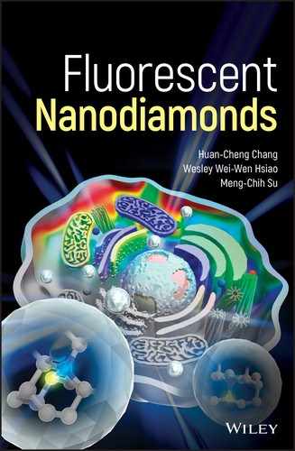
To start with, diamond is known to be radiation‐tolerated due to its “toughness.” For electron irradiation, only particles with sufficient energies are able to create vacancies in the targeted diamond materials. Campbell et al. [4, 5] have studied in detail the mechanism of radiation damage by electrons. Two major processes are involved in the damage: (i) Rutherford scattering and (ii) knock‐on atoms. Rutherford scattering is the elastic scattering of charged particles by Coulombic interactions [6]. The carbon atom in diamond can be displaced by the incident electron if, after collision, the atom has received an energy greater than what is known as the displacement energy, Edis. The typical value of Edis for diamond is 35–43 eV, which means that electrons with a kinetic energy of lower than 165–197 keV cannot cause radiation damage. A Monte Carlo program has been developed by the researchers to simulate the progress of incident electrons through diamond. In cases that the displaced carbon atom has a sufficient energy to displace further atoms (i.e. knock‐on atoms), carbon–carbon collisions should be taken into account. A well‐tested computer program, known as Transport of Ions in Matter (TRIM) [7] is available to accurately predict the distribution of the knock‐on atoms and the trail of damage left by them. Figure 6.1a displays the damage profiles of a diamond, created by electron irradiation with energies of 1, 2, and 5 MeV. The three profiles all show a sharp cut‐off (i.e. the penetration depth), as predicted by the theoretical simulations. The maximum penetration depth of the electrons increases nearly linearly with energy from 1.6, 3.0, to 7.9 mm at 1, 2, and 5 MeV, respectively (Figure 6.1b). The corresponding total vacancy production was 0.23, 0.66, and 2.23 vacancies electron−1 [4, 5].
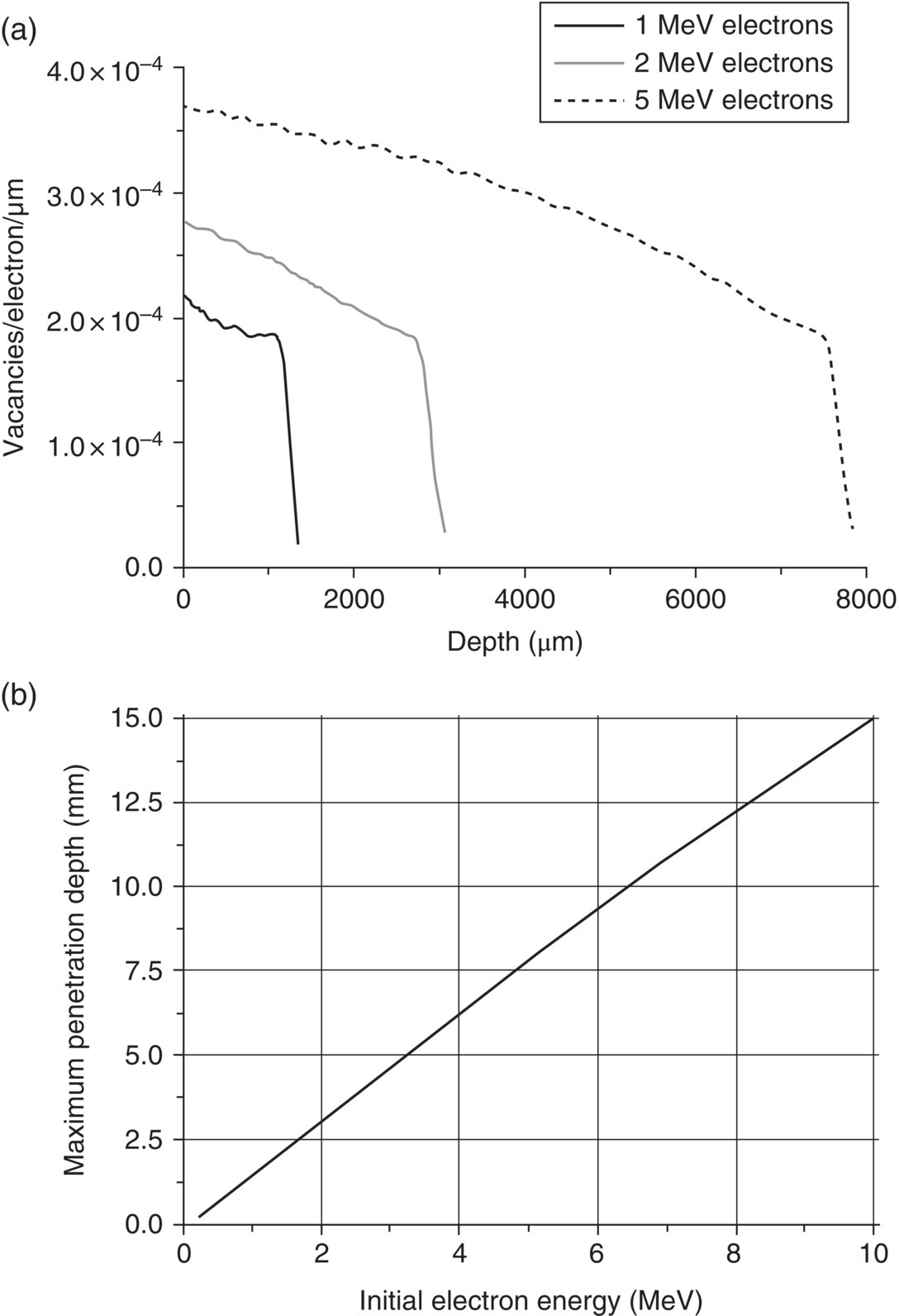
Figure 6.1 (a) Numbers of vacancies created as a function of depth by 1, 2, and 5 MeV electrons through diamond. (b) Maximum penetration depths of diamond damage as a function of electron energy.
Source: Adapted with permission from Ref. [4].
Ion irradiation is another way to create defects in the crystal structure of diamond. Similar to electron irradiation, the ion–matter collisions can be simulated with the computer program Stopping and Range of Ions in Matter (SRIM) [8], which includes the ion stopping and range tables with TRIM as the core program. The TRIM first calculates the impact and energy changes after ion–matter interactions based on the binary collision approximation [9]. The SR tables provide the stopping status and range when the ions of different energies interact with the matter. In the simulation, the types of ions (such as the simplest ion, H+) and their energies (such as 10 eV to 2 GeV) are first chosen as the input parameters. Target materials, sample thicknesses, incident angles, and combinations of different materials (if applicable) are also entered in the program.
TRIM is a Monte Carlo‐based simulation tool. When high‐energy charged particles enter the target material, the simulation tracks the trajectories of the incident particles colliding with the target material. Neglecting the impact caused by neighboring atoms, TRIM calculates the distance between two collisions and other associated parameters by random sampling. The parameters recorded during the processes include the final position, energy loss, and secondary particles, with all corresponding expectation errors analyzed statistically. The incident particles are displayed in a three‐dimensional distribution plot, effectively showing the depth of penetration. Reported in the final results are the kinetic energy produced during the collision process, the damage to the target, ionization, phonon generation, defect condition, and sputtering. The program is now widely used by researchers in the field to simulate the ion distributions of irradiation before any real experiments.
For the illustration purpose, the SRIM simulations are performed here using protons and helium ions as the damaging agents [10–15]. The values of the parameters used to carry out the simulations for both ions are all built in the software. The simulation starts with low incident energy, which is raised gradually. The selected target material is carbon, with its well‐known density of 3.52 g cm−3 and Edis of 37.5 eV for diamond. The target thickness is set as 100 μm for both ions with the energy of 0–3 MeV. The calculation time and accuracy depend on the numbers of sampling, which is typically set at 10 000. Figure 6.2a and b display, respectively, the number of vacancies produced by bombardment with these two types of ions and the corresponding maximum penetration depths. At 2 MeV, the proton has a total vacancy production yield of approximately 10 vacancies ion−1, which is 14 times that (i.e. ~0.7 vacancies electron−1) of 2‐MeV electrons, estimated from the integrated area in Figure 6.1a. However, its maximum penetration depth is only 24 μm, which is about 1/120 that of the 2‐MeV electrons. Notably, the ion distribution of the 3‐MeV protons (as well as other ions) exhibits a maximum at the region where they stop in the crystal (Figure 6.3a). The peak, known as the spread‐out Bragg peak in proton beam therapy [16], becomes sharper and more pronounced as the beam energy increases.
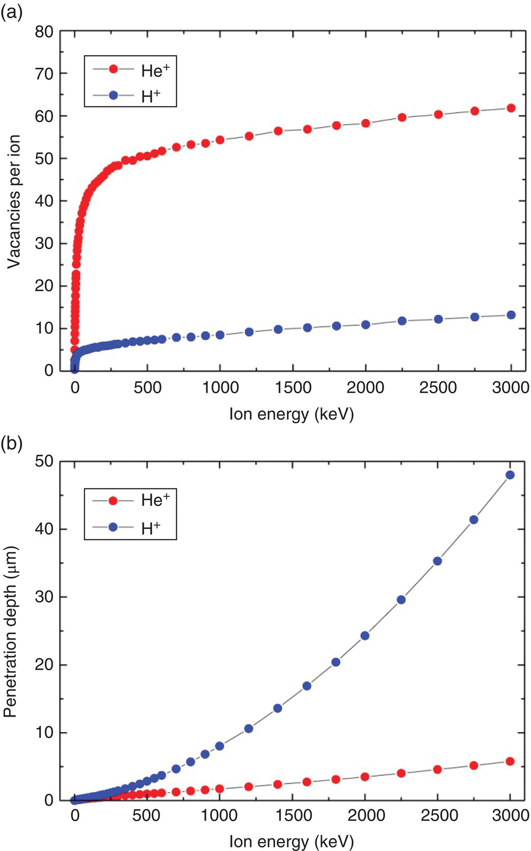
Figure 6.2 (a) Numbers of vacancies created as a function of depth by H+ and He+ ions through diamond. (b) Maximum penetration depths of diamond damage as a function of the energy of H+ and He+ ions. A displacement energy of 37.5 eV was used in the simulations.
Source: Adapted with permission from Ref. [13]. Reproduced with permission of Elsevier.
Figure 6.3 Spatial distribution of vacancies produced in diamond as a function of target depth predicted by SRIM Monte Carlo simulations. The proton beams used for the irradiation are (a) 3 MeV and (b) 40 keV, respectively. The numbers of damage events used in both simulations are 9999. Note that the vacancies are more uniformly distributed along the target depth in (b).
Source: Adapted with permission from Ref. [11]. Reproduced with permission of American Chemical Society.
6.1.2 Electron/Ion Irradiation
Now, on the experimental side, creating vacancies in diamond can be achieved by bombarding the material with high‐energy (typically 2 MeV) electrons from devices like the Van de Graaff accelerator [17]. However, the lack of easy accessibility to these research‐type accelerators makes it difficult to produce color centers in diamond on a routine basis. Another way of doing this is to use Rhodotron, a new commercial type of continuous‐wave electron accelerator that has found broad industrial applications such as sterilization of medical devices. The accelerator produces a powerful electron beam (30–200 kW) in the energy range of 1–20 MeV [18]. Boudou et al. [19, 20] first reported the use of the Rhodotron technique for high‐yield fabrication of FNDs. They fabricated fluorescent microdiamonds (FMDs) by bombarding submillimeter‐sized diamond powders with 10‐MeV electrons from the accelerator operating at a beam power of 80 kW (e.g. 10 MeV and 8 mA), followed by annealing at 800 °C. The size of the FMDs was then reduced to the sub‐100‐nm range by high‐energy air‐jet milling and ball milling. Due to the long penetration depth (up to 15 mm in Figure 6.1b) of the electrons, the FMDs (and similarly FNDs) could be readily produced on the gram scale. Figure 6.4a and b show the color change of HPHT microdiamonds before and after the electron irradiation and annealing treatment.
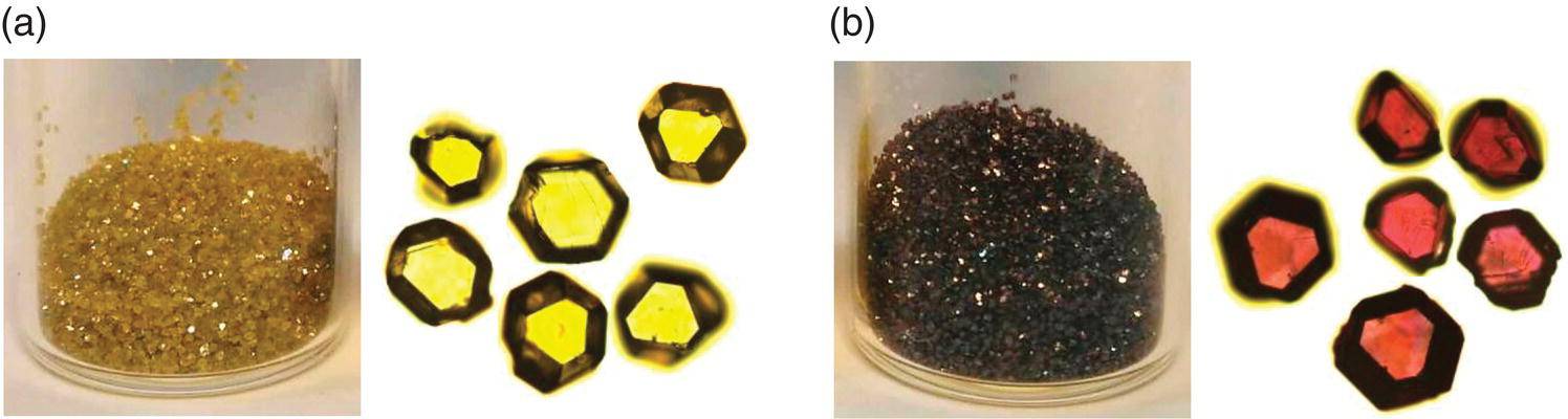
Figure 6.4 Photographs of HPHT microdiamonds before (a) and after (b) electron irradiation and thermal annealing. A bright‐field transmission image of the corresponding particles (~400 μm in diameter) is shown on the right of each panel.
While the irradiation with 10‐MeV electrons allows for scale‐up production of FNDs, they are not really suitable for daily operations because of the elaborate setup for necessary operations. Moreover, optimizing the irradiation conditions to produce the brightest FNDs is quite difficult and costly. The ion irradiation, alternatively, provides a more feasible approach since its radiation damage threshold is substantially lowered due to the much larger mass of ions compared with the electron. To maximize the penetration depth without having to use a particle accelerator, Chang and coworkers [12, 13] have employed 40‐keV protons or helium ion beams that can be readily installed and operated in any ordinary laboratory. According to the SRIM simulations (Figures 6.2 and 6.3b), each 40‐keV H+ ion will penetrate diamond by 230 nm with four vacancies created along the way. If the 40‐keV He+ ions are used instead, the penetration depth would decrease to 200 nm but the number of vacancies produced per ion can increase markedly to 40. Although the helium ion has a shallow penetration depth, it is able to penetrate through NDs of 100 nm or smaller in size without problems. It has the advantages of reducing the needed ion dose and reaction time, a feature of particular importance to achieve high vacancy densities in NDs.
Figure 6.5 shows a schematic diagram and a photograph of the experimental setup used to create vacancies in NDs. In this experiment, He+ ions are generated by radio‐frequency discharge of pure He to form a positive ion source and accelerated to 40 keV via a high‐voltage acceleration tube. The typical current of the unfocused ion beam without mass discrimination is in the 10 μA range. To cope with the small penetration depth problem, 100‐nm ND powders are first spread thin on the surface of a long copper tape before being placed in the ion implantation chamber. With the tape rotating in the chamber, all ND particles can be exposed to the ion bombardment over several cycles of treatment. Using this high‐flux ion beam facility and subsequent annealing, radiation‐damaged NDs in tens of milligram quantities can be produced on a routine basis [12].

Figure 6.5 Experimental setup used to create vacancies in NDs with a medium‐energy ion beam.
Source: Reprinted with permission from Refs. [2, 12]. Reproduced with permission of American Chemical Society.
6.1.3 Size Reduction
As discussed in Section 3.3, radiation‐damaged NDs must go through annealing to promote migration of vacancies in the diamond crystal lattice to form vacancy‐related color centers. Typically, this is performed in a vacuum at 800 °C or above for two hours. However, the annealing together with irradiation by electrons or ions inevitably results in graphitization on the diamond surface, leading to quenching of the FND fluorescence [21]. The effect becomes a serious concern for 100 nm or smaller FNDs that have large surface‐area‐to‐volume ratios. A way to overcome this problem is to oxidize the freshly prepared FNDs (i.e. right after irradiation and annealing) in air at 450 °C for one hour to remove graphitic surface structures [22], followed by washing in a concentrated H2SO4:HNO3 mixture at 100 °C to remove metal and other impurities (Figure 6.6) [23]. After separation by centrifugation and extensive rinsing in distilled deionized water, the purified FND powders can be either suspended in water or dried in air prior to use. The final size of the nanoparticles is amenable to characterization by dynamic light scattering (DLS), transmission electron microscopy (TEM), or atomic force microscopy (AFM). It is worth noting that since FNDs are prepared under such harsh conditions, the shelf lifetime of the final product is extremely long (more than one year) at room temperature.
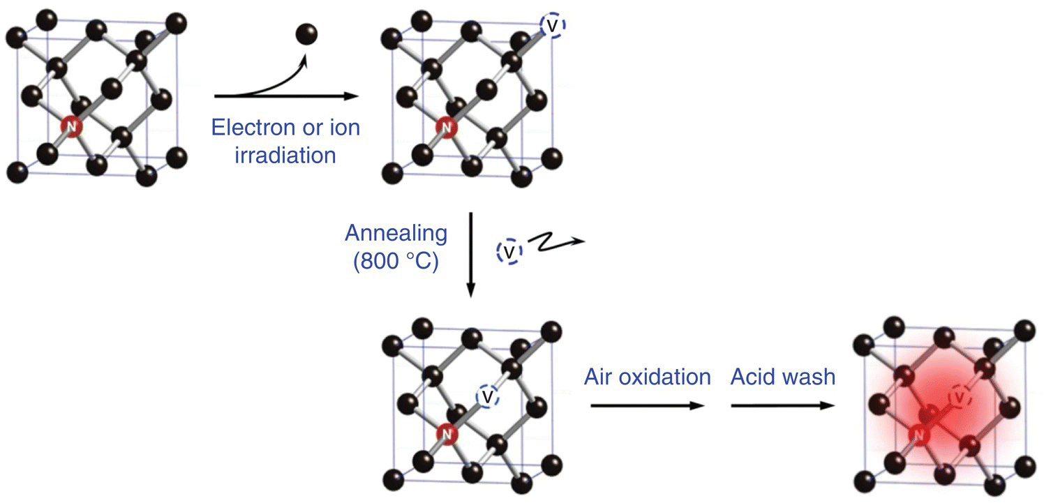
Figure 6.6 Procedures of FND production. The method is applicable for all color centers, not limited to NV as illustrated herein.
The FNDs produced by radiation damage of HPHT‐NDs usually have a broad size distribution (Figure 4.8a). They vary not only in size but also in shape from batch to batch (Figure 4.10a). For any given commercial HPHT‐ND powders with a median size of 35 nm, it is typical that one‐fifth of the particles are smaller than 20 nm. These particles can be separated and collected by differential centrifugation after optimization of the experimental conditions. The yield can be further increased by combining air oxidation and the differential centrifugation techniques. For example, Mohan et al. [24] reported a procedure to produce sub‐20‐nm FNDs based on the above two‐step approach. They first extracted sub‐20‐nm FNDs from the 50‐nm ensemble by differential centrifugation and then reduced the size of larger particles in the sample by air oxidation at 500 °C for one to two hours. Iteration of these two steps allowed the production of smaller FNDs without damaging their crystal structures. Ultimately, the method can be applied to produce FNDs down to 1 nm in size with high yields at the cost of an extended processing time [25, 26].
With the air‐oxidation method, Gaebel et al. [3] characterized in detail the size reduction and its effects on the nitrogen‐vacancy (NV) centers in unirradiated HPHT‐NDs using a combined AFM and confocal fluorescence microscope (Figure 6.7a). They found that the average height reduction rate of the individual nanocrystals, as measured by AFM, was 10 nm h−1 at 600 °C, 4 nm h−1 at 550 °C, and less than 1 nm h−1 at 500 °C by air oxidation at atmospheric pressure. The oxidation effectively removed graphitic materials from the surface, thereby reducing the background fluorescence signals. By conducting fluorescence imaging for the individual particles (Figure 6.7b and c), they observed the annihilation of NV centers on the surface, which provided important insight into the behavior of these color centers in small diamond crystallites.
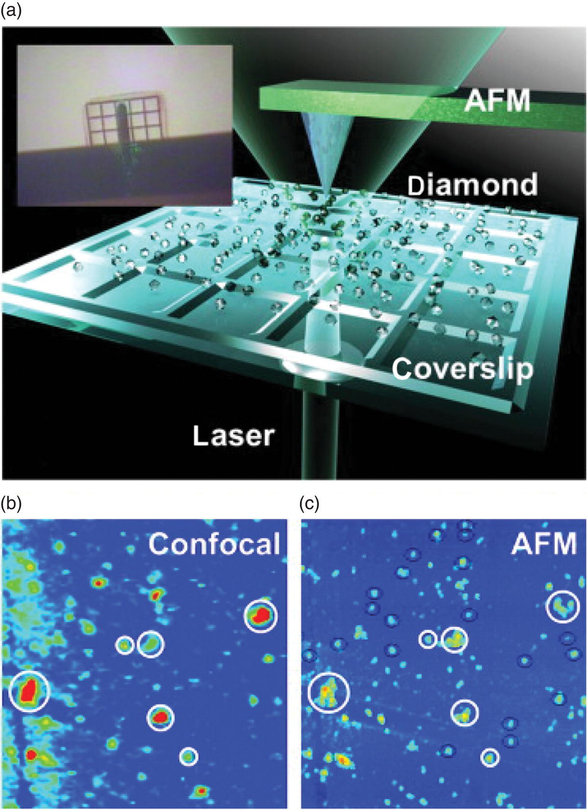
Figure 6.7 Experimental setup for the characterization of air‐oxidized NDs. (a) An artistic view of the confocal beam incident from the bottom and through the glass coverslip combined with the AFM tip probing the sample from above. The inset is a photograph of the sample from directly above. (b, c) A confocal fluorescence intensity map (b) and an AFM height map (c) of the sample. The scan area is 50 × 50 μm.
Source: Reprinted with permission from Ref. [3]. Reproduced with permission of Elsevier.
While air oxidation is a feasible approach to decrease the particle size, the yield is low and the process is time‐consuming and laborious. Another way of reducing the particle size is by high‐pressure crushing. Su et al. [27] developed such a method to produce smaller FND particles but with low damage to the crystal structures. They first mixed 30‐nm FNDs with NaF powders at a weight ratio of 1 : 10 and pressed them to form a pellet under a pressure of 10 tons by a hydraulic oil press. The pellet was then annealed at 720 °C in a vacuum for two hours, after which it was dissolved in hot water to remove NaF. The method is much gentler than ball milling and introduces almost no loss in the yield of smaller FNDs with contamination‐free quality. The yield is typically 5% for particles of less than 20 nm in diameter.
6.2 Characterization
6.2.1 Fluorescence Intensity
The final FNDs, produced by irradiation, annealing, oxidation, and acid wash treatments as described above, are now ready for fluorescence testing. Figure 6.8 shows a schematic layout of the optical setup used to acquire the fluorescence spectrum of FNDs suspended in water. The need for such a special arrangement is because diamond has a high refractive index (n = 2.41 in the visible region), which causes strong light scattering at the diamond–water interfaces. The scattering can seriously distort the observed spectra if the fluorescence is collected and detected with a CCD‐based spectrophotometer in a perpendicular geometry. Displayed in Figure 6.9 are typical fluorescence spectra of green and red FNDs excited by 473‐ and 532‐nm laser light, respectively. The fluorescence intensity of each sample provides a relative measure for the density of vacancy‐related color centers in the diamond matrix. The results of the measurements serve as an important guide to the production of brighter FNDs through adjusting the doses of electron or ion irradiation.

Figure 6.8 Optical layout of the experimental setup for fluorescence measurements of red FNDs suspended in water. A round electromagnet supplies a time‐varying magnetic field of 0–50 mT, as controlled by a power amplifier. By changing the laser and optics, the setup can be applied to detect FNDs containing other color centers such as H3.
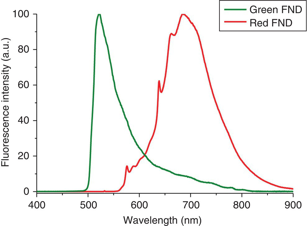
Figure 6.9 Fluorescence spectra of H3 and NV centers in green and red FNDs, respectively, suspended in water. The sizes of both particles are approximately 100 nm in diameter and the FND concentration is 1 mg ml−1 each.
The optical properties of FNDs can be further characterized by depositing them on a glass slide for fluorescence imaging. Bright‐field imaging of the red FNDs produced by 3‐MeV proton irradiation of HPHT‐NDs showed that these particles formed aggregates on the glass slide when dried in air (Figure 6.10a). Excitation of the FNDs with the yellow lines from a 100 W mercury vapor lamp produced intense red emission (Figure 6.10b). The fluorescence intensity was nearly two orders of magnitude higher than that of the samples without irradiation but with annealing under the same conditions. No sign of photobleaching was observed for the FND even after eight hours of continuous excitation with the Hg lamp (Figure 6.10c). In contrast, the 0.1‐μm red fluorescent polystyrene nanospheres containing approximately 104 dye equivalents photobleached within 0.5 hour when excited by the same lamp light [1]. The high photostability was similarly observed for green FNDs excited with the mercury lamp light at 450–490 nm [13].
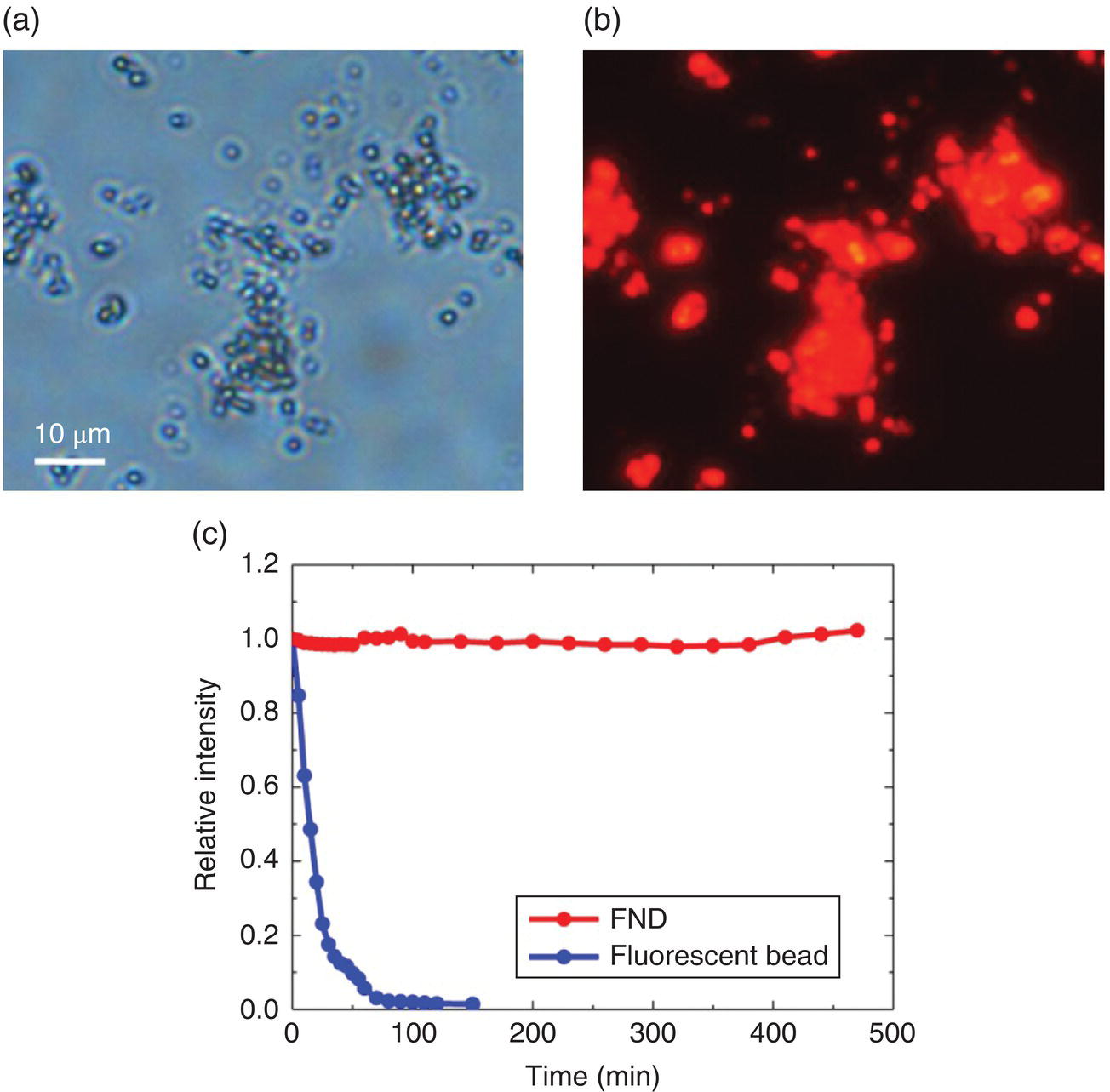
Figure 6.10 (a) Bright field and (b) epifluorescence images of red FNDs. Both images were obtained with a 40× objective. (c) Photostability tests of FND (red) and fluorescent polystyrene beads (blue) excited under the same conditions. The excitation was made with light of 510–560 nm in wavelength.
Source: Reprinted with permission from Ref. [1]. Reproduced with permission of American Chemical Society.
6.2.2 Electron Spin Resonance
A question often asked is: What is the density of NV or H3 centers in the FNDs? According to the SRIM Monte Carlo simulations, a 3‐MeV proton will produce 12 vacancies when penetrating diamond (Figure 6.2). The penetration depth is approximately 50 μm. If a dose of 1 × 10¹⁶ ions cm−2 is used for irradiation, the density of the vacancies created in the crystals is 2.4 × 10¹⁹ centers cm−3 (equivalent to 140 ppm, where 1 ppm = 1.76 × 10¹⁷ carbon atoms cm−3 for diamond), corresponding to the production of 1.2 × 10⁴ vacancies per 100‐nm particle. This amount of vacancies is of the same magnitude as that of nitrogen atoms in each 100‐nm HPHT‐ND. Assuming that the efficiency of the NV− production is 10%, similar to that found for bulk diamonds [28], the number of NV− centers in the individual 100‐nm FNDs, made of HPHT‐NDs, is on the order of 103 or a density of approximately 10 ppm [1, 28]. The number agrees in the ballpark with that reported by Wee et al. [11] who bombarded type Ib bulk diamonds with a 3‐MeV proton beam from a tandem accelerator and determined a NV− density in the range of 25 ppm.
A direct measurement for the number of NV− centers can be accomplished with electron spin resonance (ESR) spectroscopy [29]. Shames et al. [30] applied the technique to track the multistage process of the fabrication of FNDs produced by high‐energy electron irradiation, annealing, and subsequent milling of type Ib diamond microcrystals (Figure 6.4). Their results indicated that the irradiation with 10‐MeV electrons and subsequent annealing of the irradiated microdiamonds at 800 °C could produce triplet magnetic centers, identified as NV−, with a density up to 5.4 × 10¹⁷ spins g−1 (or 1.9 × 10¹⁸ spins cm−3 or 11 ppm). However, after progressive milling of the FMDs down to a submicron scale, the relative abundance of NV− in the final product was reduced to 3.6 × 10¹⁷ spins g−1 (or 7.2 ppm), corresponding to 660 NV− centers in each 100‐nm FND particle. Although increasing the nitrogen content in the type Ib microdiamonds could facilitate the production of NV− centers, it also introduced structural imperfections, which were responsible for the appearance of additional nonradiative recombination centers in the ESR spectra and fluorescence quenching [31].
6.2.3 Fluorescence Lifetime
Fluorescence lifetime is another significant photophysical property of FNDs. For the NV− centers in bulk type Ib diamond, the lifetime of the 3E → 3A2 transition (Figure 3.8) is 11.6 ns as well‐documented in the literature [32]. However, the lifetime can be significantly altered if the crystal size becomes smaller than the wavelength of the excitation light. It is known that for a molecular fluorophore in solution, its radiative decay rate is proportional to the square of the refractive index (n2) of the environment due to the change in polarizability [33]. Although such a refractive index is not well defined for FNDs in water (n = 1.33), it is clearly smaller than that of bulk diamond (n = 2.41). So, one can expect a decrease of the radiative decay rate or an increase of the fluorescence lifetime for the color centers in FNDs.
Figure 6.11a displays typical fluorescence decay time traces of two red FND samples (100 and 35 nm in size) in water. Unlike the single‐exponential decay observed for the NV− centers in bulk diamond, both the fluorescence time traces should be fitted with two decay constants:

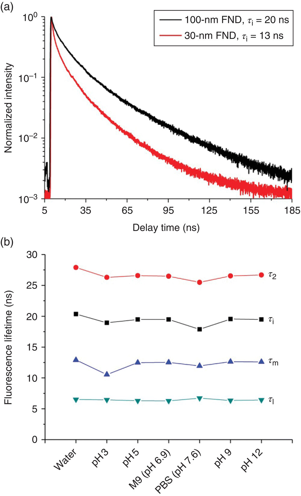
Figure 6.11 (a) Comparison of the fluorescence lifetimes of FNDs with different sizes (100 and 30 nm in diameter). The concentration of both FND suspensions is 1 mg ml−1. (b) Variation of the fluorescence lifetimes of 100‐nm FNDs in water, biological buffer, and aqueous solutions with different pHs. The amplitude‐weighted mean lifetime (τm) and the intensity‐weighted mean lifetime (τi) are calculated from τ1 and τ2 according to Eqs. (6.2) and (6.3) in text.
The observation of such a characteristic double‐exponential decay is presumably due to the presence of a high‐density ensemble (~10 ppm) of NV− centers in each FND particle that complicates the energy relaxation dynamics. The amplitude‐weighted mean lifetime (τm) is

and the intensity‐weighted mean lifetime (τi) is
Both lifetimes vary with the sample size; for example, the value of τi decreases from 20 ns of 100‐nm FNDs to 13 ns of 30‐nm FNDs [27]. The shortening of the observed lifetime (τobs) could be attributed to fluorescence quenching by surface defects [34], as the fluorescence quantum yield (QF) is related to the intrinsic radiative rate constant (kr) and the nonradiative rate constant (knr) by
Such a surface effect is expected to play a more significant role as the particle size decreases. The effect is particularly pronounced for DNDs, which are approximately 5 nm in diameter with a graphitic shell coated on the surface [35, 36]. As a result, DNDs are only weakly fluorescent and the emission is not photostable [37].
Described in the previous section, the density of NV− centers in the 100‐nm FNDs may be as high as 10 ppm. Assuming that these centers are uniformly distributed in the diamond lattice, the nearest neighbors are separated by roughly 10 nm. While most of the centers are embedded deeply in the crystal matrix, some of them are located within a 5‐nm thickness of the outer surface shell, where their fluorescence properties can be significantly influenced by the external environment. Figure 6.11b shows how the fluorescence lifetimes of 100‐nm FNDs are varied when they are suspended in water, biological buffer, and aqueous solutions with different pH values. All the fluorescence time traces exhibit double‐exponential decay characteristic with a fast component of τ1 ~ 6 ns and a slow component of τ2 ~ 26 ns. Even under the extreme conditions of pH 3 and 12, the lifetime is virtually unchanged, revealing the exceptionally high chemical stability of the nanomaterial and the hosted color centers [38]. The result suggests that all the surface chemistry described in Chapter 4 will have only a minor effect on the fluorescence properties of the NV− centers as long as the size of FNDs is maintained in the neighborhood of 100 nm. The same principle applies for the H3 centers in green FNDs of comparable size.
6.2.4 Magnetically Modulated Fluorescence
We now turn to the magnetic properties of NV− centers in FNDs. As explained in Section 3.4, the NV− center is unique in that it has two unpaired spins, exhibiting a magnetic resonance at 2.87 GHz (∆ms = 0 → ±1) in the ground electronic state. Interestingly, the spin states of NV− can be optically polarized after several cycles of electronic excitation [39]. In the presence of an external magnetic field, not in alignment with the NV symmetry axis, the fluorescence intensity would decrease because the magnetic field lifts the degeneracy of the ms = ±1 sublevels and mixes them with the ms = 0 sublevel (Figure 3.8). For an ensemble of NV− centers in bulk diamond, a change of the fluorescence intensity by more than 10% can result [40, 41]. Exploiting this unique magneto‐optical property, Chapman and Plakhotnik [42] were able to achieve background‐free imaging of FNDs on a glass slide by switching an external magnetic field on and off, followed by subtraction of the signals from these two measurements for contrast enhancement. The method is particularly suitable for detecting NV− in high backgrounds. The magnetic modulation, though less common than optical modulation, has the advantage of being more applicable to samples with strong light scattering and complex chemical compositions [43].
The feasibility of modulating the fluorescence intensity of NV− has also been tested for FNDs in solution (cf., Figure 6.8 for the experimental setup). Figure 6.12a displays a typical fluorescence spectrum of 100‐nm FNDs suspended in water (concentration of 1 mg ml−1) and excited by a 532‐nm laser. The fluorescence intensity showed a maximum at 687 nm with a modulation depth of approximately 5% when the particles were exposed to a time‐varying magnetic field with a strength of B = 20 mT at an on/off switching frequency of f = 2 Hz (Figure 6.12b). However, as the FND concentration was lowered to 1 μg ml−1 or less, the NV− emission could not be seen because the Raman signals of water dominated the observed spectrum. Luckily, the Raman signals were not affected by the magnetic modulation, thereby allowing removal of the background signals by fast Fourier transform (FFT) of the time traces using a computer program for frequency demodulation at each wavelength [44]. As shown in Figure 6.12c, the fluorescence signal of a highly diluted FND solution (concentration ~0.1 μg ml−1) was originally overwhelmed by the water Raman peaks; the background level, however, could be effectively reduced by more than two orders of magnitude with the magnetic modulation technique.
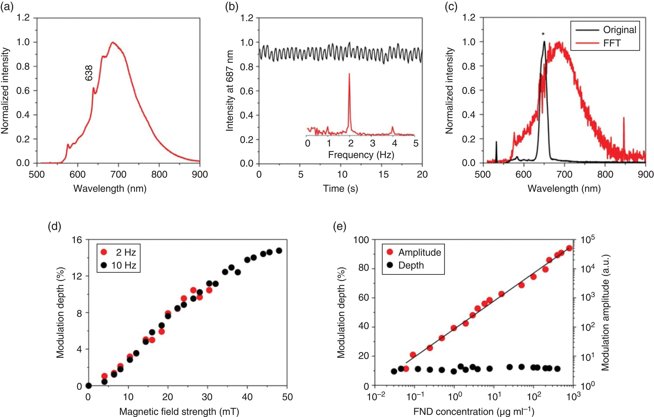
Figure 6.12 Ultrasensitive quantification of FNDs by magnetically modulated fluorescence. (a) Normalized fluorescence spectrum of FNDs in water (1 mg ml−1), excited with a 532 nm laser. (b) Time trace of the peak fluorescence intensity at 687 nm under magnetic modulation at f = 2 Hz. The inset shows the corresponding frequency spectrum after FFT. (c) Normalized fluorescence spectrum of FNDs (0.1 μg ml−1) in water (black) and its FFT spectrum (red) after demodulation at f = 2 Hz. The asterisk denotes the Raman peaks of water. (d) Dependence of fluorescence modulation depth on the magnetic field strength at f = 2 and 10 Hz for FNDs in water (0.1 mg ml−1). (e) Demodulated fluorescence intensity of FNDs as a function of the particle concentration at f = 10 Hz and B = 40 mT. Solid line is a linear fit of the experimental data. Note that the magnetic modulation depth is independent of the FND concentration even when the concentration is as low as 60 ng ml−1.
Source: Adapted with permission from Ref. [44].
In a recent study, our group has also investigated how the modulation depth of the NV− emission depends on the magnetic field strength. Instead of obtaining the whole emission spectra, we collected the total fluorescence signals at 650–750 nm using a bandpass filter and an avalanche photodiode as the detector. Figure 6.12d shows the modulation depth of the signals as a function of the magnetic field strength varying sinusoidally at 2 and 10 Hz. The depth increased with B and gradually reached a plateau (~15%) when B ≥ 50 mT. With the instrument operating at B = 40 mT, f = 10 Hz, and a data acquisition time of 10 seconds, a detection limit as low as 60 ng ml−1 was readily achieved (Figure 6.12e). Assuming a spherical shape for the FND particles, the lowest detectable concentration was estimated to be 50 fM or 3 × 10⁷ particles ml−1.
Finally, it is worth noting that background‐free detection by optically modulated fluorescence can also be achieved with FNDs. Using a green laser to drive the electronic transition of the NV− centers in bulk diamond, Geiselmann et al. [45] reported an optical modulation of more than 80% and a time response of faster than 100 ns, controlled by a near‐infrared gating laser, which promoted the population in the excited state (3E) to an unknown dark band. Compared with magnetically modulated fluorescence, the method is advantageous in having a larger modulation depth and a faster modulation rate. It is compatible with optical lock‐in detection fluorescence microscopy [46, 47], a technique developed to enhance the image contrast of fluorescent proteins or fluorescently labeled biomolecules in living cells by intensity modulation. Both the optical and magnetic modulation methods are ideally suited for high sensitivity detection of FNDs in extremely dilute solutions as well as high selectivity imaging of FNDs in complex biological environments as discussed in Chapter 9.
References
- 1 Yu, S.J., Kang, M.W., Chang, H.C. et al. (2005). Bright fluorescent nanodiamonds: no photobleaching and low cytotoxicity. J Am Chem Soc 127: 17604–17605.
- 2 Hsiao, W.W.W., Hui, Y.Y., Tsai, P.C., and Chang, H.C. (2016). Fluorescent nanodiamond: a versatile tool for long‐term cell tracking, super‐resolution imaging, and nanoscale temperature sensing. Acc Chem Res 49: 400–407.
- 3 Gaebel, T., Bradac, C., Chen, J. et al. (2011). Size‐reduction of nanodiamonds via air oxidation. Diam Relat Mater 21: 28–32.
- 4 Campbell, B. and Mainwood, A. (2000). Radiation damage of diamond by electron and gamma irradiation. Physica Stat Sol A 181: 99–107.
- 5 Campbell, B., Choudhury, W., Mainwood, A. et al. (2002). Lattice damage caused by the irradiation of diamond. Nucl Instrum Meth A 476: 680–685.
- 6 Halliday, D., Walker, J., and Resnick, R. (2010). Fundamentals of Physics, 5e. New York: Wiley.
- 7 Biersack, J.P. and Haggmark, H.G. (1980). A Monte Carlo computer program for the transport of energetic ions in amorphous targets. Nucl Instr Meth 174: 257–269.
- 8 Ziegler, J.F., Biersack, J.P., and Littmark, U. (1985). The stopping and range of ions in solids. Pergamon. www.srim.org (accessed 16 April 2018).
- 9 Robinson, M.T. and Torrens, I.M. (1974). Computer simulation of atomic‐displacement cascades in solids in the binary‐collision approximation. Phys Rev B 9: 5008–5024.
- 10 Waldermann, F.C., Olivero, P., Nunn, J. et al. (2007). Creating diamond color centers for quantum optical applications. Diam Relat Mater 16: 1887–1895.
- 11 Wee, T.L., Tzeng, Y.K., Han, C.C. et al. (2007). Two‐photon excited fluorescence of nitrogen‐vacancy centers in proton‐irradiated type Ib diamond. J Phys Chem A 111: 9379–9386.
- 12 Chang, Y.R., Lee, H.Y., Chen, K. et al. (2008). Mass production and dynamic imaging of fluorescent nanodiamonds. Nat Nanotechnol 3: 284–288.
- 13 Wee, T.L., Mau, Y.W., Fang, C.Y. et al. (2009). Preparation and characterization of green fluorescent nanodiamonds for biological applications. Diam Relat Mater 18: 567–573.
- 14 Acosta, V.M., Bauch, E., Ledbetter, M.P. et al. (2009). Diamonds with a high density of nitrogen‐vacancy centers for magnetometry applications. Phys Rev B 80: 115202.
- 15 Botsoa, J., Sauvage, T., Adam, M.P. et al. (2011). Optimal conditions for NV‐ center formation in type‐1b diamond studied using photoluminescence and positron annihilation spectroscopies. Phys Rev B 84: 125209.
- 16 Levin, W.P., Kooy, H., Loeffler, J.S., and DeLaney, T.F. (2005). Proton beam therapy. Br J Cancer 93: 849–854.
- 17 Davies, G., Lawson, S.C., Collins, A.T. et al. (1992). Vacancy‐related centers in diamond. Phys Rev B 46: 13157–13170.
- 18 Jongen, Y., Abs, M., Capdevila, J.M. et al. (1994). The Rhodotron, a new high‐energy, high‐power, CW electron accelerator. Nucl Instrum Meth B 89: 60–64.
- 19 Boudou, J.P., Curmi, P.A., Jelezko, F. et al. (2009). High yield fabrication of fluorescent nanodiamonds. Nanotechnology 20: 235602.
- 20 Boudou, J.P., Tisler, J., Reuter, R. et al. (2013). Fluorescent nanodiamonds derived from HPHT with a size of less than 10 nm. Diam Relat Mat 37: 80–86.
- 21 Smith, B.R., Gruber, D., and Plakhotnik, T. (2010). The effects of surface oxidation on luminescence of nanodiamonds. Diam Relat Mater 19: 314–318.
- 22 Osswald, S., Yushin, G., Mochalin, V. et al. (2006). Control of sp2/sp3 carbon ratio and surface chemistry of nanodiamond powders by selective oxidation in air. J Am Chem Soc 128: 11635–11642.
- 23 Huang, L.C.L. and Chang, H.C. (2004). Adsorption and immobilization of cytochrome c on nanodiamonds. Langmuir 20: 5879–5884.
- 24 Mohan, N., Tzeng, Y.K., Yang, L. et al. (2010). Sub‐20‐nm fluorescent nanodiamonds as photostable biolabels and fluorescence resonance energy transfer donors. Adv Mater 22: 842–847.
- 25 Stehlik, S., Varga, M., Ledinsky, M. et al. (2015). Size and purity control of HPHT nanodiamonds down to 1 nm. J Phys Chem C 119: 27708–27720.
- 26 Stehlik, S., Varga, M., Ledinsky, M. et al. (2016). High‐yield fabrication and properties of 1.4 nm nanodiamonds with narrow size distribution. Sci Rep 6: 38419.
- 27 Su, L.J., Fang, C.Y., Chang, Y.T. et al. (2013). Creation of high density ensembles of nitrogen‐vacancy centers in nitrogen‐rich type Ib nanodiamonds. Nanotechnology 24: 315702.
- 28 Pezzagna, S., Naydenov, B., Jelezko, F. et al. (2010). Creation efficiency of nitrogen‐vacancy centres in diamond. New J Phys 12: 065017.
- 29 Atherton, N.M. (1993). Principles of Electron Spin Resonance. PTR Prentice Hall, Ellis Horwood.
- 30 Shames, A.I., Yu Osipov, V., Boudou, J.P. et al. (2015). Magnetic resonance tracking of fluorescent nanodiamond fabrication. J Phys D: Appl Phys 155302: 48.
- 31 Shames, A.I., Osipov, V.Y., Bogdanov, K.V. et al. (2017). Does progressive nitrogen doping intensify negatively charged nitrogen vacancy emission from e‐beam‐irradiated Ib type high‐pressure‐high‐temperature diamonds? J Phys Chem C 121: 5232–5240.
- 32 Collins, A.T., Thomaz, M.F., and Jorge, M.I.B. (1983). Luminescence decay time of the 1.945 eV center in type 1b diamond. J Phys C Solid State 16: 2177–2181.
- 33 Strickler, S.J. and Berg, R.A. (1962). Relationship between absorption intensity and fluorescence lifetime of molecules. J Chem Phys 37: 814–822.
- 34 Chen, L.H., Lim, T.S., and Chang, H.C. (2012). Measuring the number of (N‐V)− centers in single fluorescent nanodiamonds in the presence of quenching effects. J Opt Soc Am B 29: 2309–2313.
- 35 Bradac, C., Gaebel, T., Naidoo, N. et al. (2010). Observation and control of blinking nitrogen‐vacancy centres in discrete nanodiamonds. Nat Nanotechnol 5: 345–349.
- 36 Smith, B.R., Inglis, D.W., Sandnes, B. et al. (2009). Five‐nanometer diamond with luminescent nitrogen‐vacancy defect centers. Small 5: 1649–1653.
- 37 Vlasov, I.I., Shenderova, O., Turner, S. et al. (2010). Nitrogen and luminescent nitrogen‐vacancy defects in detonation nanodiamond. Small 6: 687–694.
- 38 Kuo, Y., Hsu, T.Y., Wu, Y.C. et al. (2013). Fluorescence lifetime imaging microscopy of nanodiamonds in vivo. Proc SPIE 8635: 863503.
- 39 Gruber, A., Drabenstedt, A., Tietz, C. et al. (1997). Scanning confocal optical microscopy and magnetic resonance on single defect centers. Science 276: 2012–2014.
- 40 Lai, N.D., Zheng, D., Jelezko, F. et al. (2009). Influence of a static magnetic field on the photoluminescence of an ensemble of nitrogen‐vacancy color centers in a diamond single‐crystal. Appl Phys Lett 95: 133101.
- 41 Rondin, L., Tetienne, J.P., Hingant, T. et al. (2014). Magnetometry with nitrogen‐vacancy defects in diamond. Rep Prog Phys 77: 056503.
- 42 Chapman, R. and Plakhotnik, T. (2013). Background‐free imaging of luminescent nanodiamonds using external magnetic field for contrast enhancement. Opt Lett 38: 1847–1849.
- 43 Yang, N. and Cohen, A.E. (2010). Optical imaging through scattering media via magnetically modulated fluorescence. Opt Express 18: 25461–25467.
- 44 Su, L.J., Wu, M.H., Hui, Y.Y. et al. (2017). Fluorescent nanodiamonds enable quantitative tracking of human mesenchymal stem cells in miniature pigs. Sci Rep 7: 45607.
- 45 Geiselmann, M., Marty, R., García de Abajo, F.J., and Quidant, R. (2013). Fast optical modulation of the fluorescence from a single nitrogen‐vacancy centre. Nat Phys 9: 785–789.
- 46 Marriott, G., Mao, S., Sakata, T. et al. (2008). Optical lock‐in detection imaging microscopy for contrast‐enhanced imaging in living cells. Proc Natl Acad Sci USA 105: 17789–17794.
- 47 Hsiang, J.C., Jablonski, A.E., and Dickson, R.M. (2014). Optically modulated fluorescence bioimaging: visualizing obscured fluorophores in high background. Acc Chem Res 47: 1545–1554.
- 48 Dantelle, G., Slablab, A., Rondin, L. et al. (2010). Efficient production of NV colour centres in nanodiamonds using high‐energy electron irradiation. J Lumin 130: 1655–1658.
- 49 Havlik, J., Petrakova, V., Rehor, I. et al. (2013). Boosting nanodiamond fluorescence: towards development of brighter probes. Nanoscale 5: 3208–3211.
- 50 Mahfouz, R., Floyd, D.L., Peng, W. et al. (2013). Size‐controlled fluorescent nanodiamonds: a facile method of fabrication and color‐center counting. Nanoscale 5: 11776–11782.
- 51 Sotoma, S., Yoshinari, Y., Igarashi, R. et al. (2014). Effective production of fluorescent nanodiamonds containing negatively‐charged nitrogen‐vacancy centers by ion irradiation. Diam Relat Mater 49: 33–38.