
The collected monitoring data can be very useful, but you probably want to use it in a more flexible way than just staring at the custom report included in the GeoServer interface.
Reports can be designed to show usage stats or check the safety state of your server. You can group them in several ways, as with any other source of alphanumerical data. There are several different tools you can use for this, most of them coming from the business intelligence, data warehousing, and analytics branches of Information Technology.
In this recipe, we want to focus again on the spatial component of the data. You may wonder what the most queried area of your datasets is, for example, and want analyze whether there are some preferential areas where your user browses for data. This may prove useful in order to tune your GeoServer for better performance, and it'll be more useful if a wider extent is covered by your data.
We'll create a point layer from the request by taking the centroid of envelopes, and then render it as Heatmap.
- Open a shell console and connect to the database where GeoServer stores the monitoring information, as follows:
$ psql -U gisuser -d gisdata - Execute the following script to create a new table from the existing information:
create table heatmap as select name, crs, service, operation, ST_Centroid(ST_GeomFromText('POLYGON((' || minx || ' ' || maxy || ',' || maxx || ' ' || maxy || ',' || maxx || ' ' || miny || ',' || minx || ' ' || miny || ',' || minx || ' ' || maxy || '))', 4326)) as geom from request join request_resources on (request_id = id) where crs is not null; - Execute the following SQL statement to create a spatial index on the new table:
CREATE INDEX heatmap_geom_gist ON public.heatmap USING gist(geom);
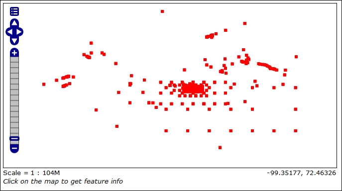
- Now open the GeoServer interface and publish the table as a new layer. Then, go to the Layer preview and check what your map shows. It shows many points, each corresponding to a request, as shown in the following screenshot:
- Now take
the ch08_heatmap.sldfile from the code accompanying this chapter and create a new GeoServer style with it. Then, change the configuration for the Heatmap layer, assigning the new style as its default. - Take the
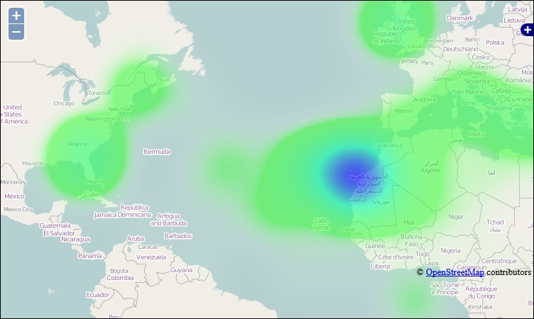
ch08_heatmapWMS.htmlfile and save it in the<CATALINA_HOME>/webapps/ROOTfolder, and then point your browser to the following URL:http://localhost:8080/ch08_heatmapWMS.html - Now the map shows you the area where concentrated requests are in blue and turn to light green as the density of the requests decreases, as shown in the following screenshot:
In this recipe, we simulated a very minimalistic data warehouse. We selected a set of information, transformed it, and created a new dataset. This is usually done with an ETL procedure, and our SQL query may be considered a very simple Extract, Transform, and Load (ETL) procedure.
Note
ETL is used to process data from a data source to another. If this is totally new to you, a good starting point might be here:
http://en.wikipedia.org/wiki/Extract,_transform,_load
General purpose ETL tools are not usually spatially aware, but in the last few years, a few robust solutions have been developed. Among proprietary solutions, the champion is Feature Manipulation Engine (FME) by Safe, which is available at http://www.safe.com/fme/.
An open source solution is GeoKettle, which is available at http://www.spatialytics.org/projects/geokettle/.
The key transformation we did to the data is to create its geometry from the numeric description of bounding boxes:
ST_Centroid(ST_GeomFromText('POLYGON((' || minx || ' ' || maxy || ',' || maxx || ' ' || maxy || ',' || maxx || ' ' || miny || ',' || minx || ' ' || miny || ',' || minx || ' ' || maxy || '))', 4326)) as geomConcatenating the minx, miny, maxx, and maxy values properly, we build a polygon, actually a rectangular shape, and then we ask PostGIS to calculate its barycenter and set this as the geometric property of the request. For instance, have a look at the following request:
    minx   |    miny    |    maxx    |    maxy    |    crs    |
-181.80000 | -90.868171 | 181.800013 | 84.5022735 | EPSG:4326
The preceding request produces the following polygon:
POLYGON((-181.800003051758 84.5022735595703,181.800018310547 84.5022735595703,181.800018310547 -90.8681716918945,-181.800003051758 -90.8681716918945,-181.800003051758 84.5022735595703))
Polygon's barycenter is shown as follows:
POINT(7.6293944864863e-06 -3.1829490661621)
The other transformation on the data is on the rendering side.
In fact, we used the rendering transformation capability of GeoServer to transform a vector data, the point layer, in a raster map. The transformation is inside the style:
…
      <Abstract>A heatmap for monitoring data</Abstract>
      <FeatureTypeStyle>
        <Transformation>
         <ogc:Function name="gs:Heatmap">
           <ogc:Function name="parameter">
             <ogc:Literal>data</ogc:Literal>
           </ogc:Function>
…
Here, we refer to the gs:Heatmap process, which is a function delivered by the WPS extension, which creates the raster data according to the point density. We used the WPS extension in Chapter 4, Geoprocessing; consult it for instructions about its installation and configuration.
The other core information delivered by the style is the color ramp used to represent the point density. We use a RasterSymbolizer element where you can customize a set of classes with color and the associated quantity, as follows:
…
          <RasterSymbolizer>
            <Geometry>
              <ogc:PropertyName>geom</ogc:PropertyName>
            </Geometry>
            <Opacity>0.6</Opacity>
            <ColorMap type="ramp" >
              <ColorMapEntry color="#FFFFFF" quantity="0"    label="nodata" opacity="0" />
              <ColorMapEntry color="#44FF44" quantity=".05"   label="nodata" />
              <ColorMapEntry color="#00FFAA" quantity=".45"   label="values" />
              <ColorMapEntry color="#0000FF" quantity="1.0"  label="values" />
            </ColorMap>
          </RasterSymbolizer>
…
Note
You can read about the details of rendering transformations available in GeoServer from the official documentation available at http://docs.geoserver.org/stable/en/user/styling/sld-extensions/rendering-transform.html.
You learned how to use the default reports to display the monitoring information, and how to create a custom report by directly accessing the database.
GeoServer also offers you a simple HTTP API to retrieve the monitoring information. This will prove very useful if you have to integrate reports in an external application that may not be comfortable accessing the database, for instance, a web application running on a remote system.
The basic form of the request is shown as follows:
http://<host>:<port>/geoserver/rest/monitor/requests.<format>
The basic request lets you get all the information formatted according to your choice. The options available for the format parameters are:
- HTML
- ZIP
- CSV
- XLS
For instance, if you send an HTTP GET request to obtain all the requests formatted in HTML, the right syntax is as follows:
$ curl –XGET http://localhost:8080/geoserver/rest/monitor/requests.html -O requests.html
The requests.html file will contain all the requests collected since GeoServer started. When you open the file in a browser, you'll have a list of data sources, as shown in the following screenshot:
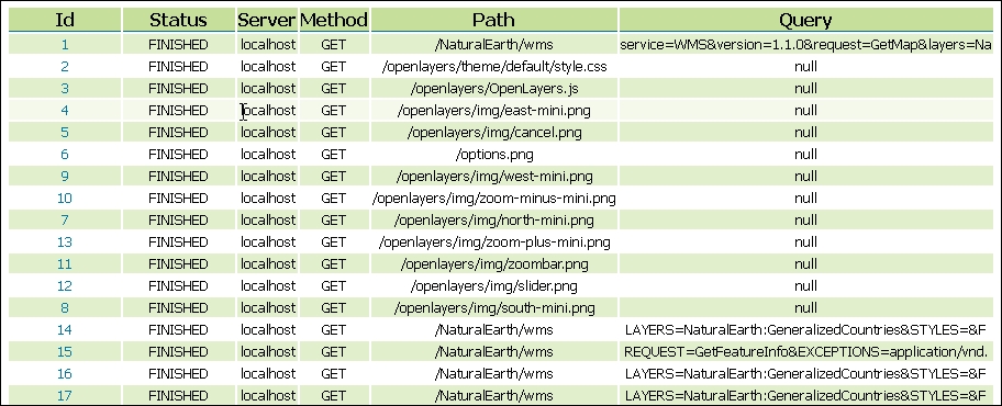
As you can see, not all fields are returned. Be aware that the previous request will return all the records in the monitoring repository, so the resulting output can be very huge.
A few options help to filter and sort the output according to your needs. You can display the output by using the count and offset parameters, if you send the following request:
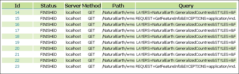
$ curl –XGET http://localhost:8080/geoserver/rest/monitor/requests.html?count=10&offset=13 –O requests.html
Now, you'll obtain a short list of 10 items starting from the 14th ID, as shown in the following screenshot:
Another option to filter the resulting set is to send a time range. There are two available parameters, from and to, and both require a timestamp, as shown in the following example, where all requests for the 24th of June are requested:
$ curl –XGET http://localhost:8080/geoserver/rest/monitor/requests.html?from=2014-06-26T00:00:00&to=2014-06-26T24:00:00 –O requests.html
If you need more information about a single request, you can send a specific request using the internal identifier, that is, use the ID as a filter:
$ curl –XGET http://localhost:8080/geoserver/rest/monitor/requests/13.html –O requests.html