
Chapter 6
Evaluating Exposures
6.1 Introduction
The human health risk associated with a chemical is dependent on the rate at which the chemical is released, the fate of the chemical in the environment, human exposure to the chemical, and human health response resulting from exposure to the chemical. In simpler terms, as described in Chapter 2, risk is a function of hazard (or toxicity) and exposure. Chapter 5 discusses methods of predicting physical-chemical properties from chemical structure to infer the fate of a chemical in the environment. Chapter 7 discusses green chemistry techniques to select chemicals that are less toxic. Chapters 5 and 7 are useful in designing chemical structures with low hazard, one of the two components of the risk equation. This chapter, Chapter 6, addresses the exposure component of the risk equation. Ideally, exposure is quantified by monitoring the work area or environmental setting where a chemical will be used or released; however, when monitoring data are not available to measure exposures, exposures can be estimated using methods described in this chapter.
The methods for estimating exposure will be separated into two sections—occupational and community. Occupational exposure occurs in the workplace. Workers in chemical production facilities may be exposed to toxins used or produced in the chemical process. Exposure to chemicals may occur from the inhalation of workplace air, ingestion of dust or contaminated food, or from contact of the chemical substance with the skin or eyes. In addition, chemical engineers must be aware of community exposures resulting from releases into the air and water, and from solid and hazardous waste disposal. Chemical releases to rivers, lakes, and streams may accumulate in fish and other marine life, which are subsequently used as a source of food, or may be ingested by persons using the downstream reaches of rivers as a supply of potable water. Persons living downwind of a chemical manufacturing facility may be exposed to fugitive and point source releases of chemical toxins to the atmosphere. Disposal of solid and hazardous wastes on the land, either in repositories such as landfills or into subterranean strata by injection into wells may result in contamination of potable groundwater if the waste is not isolated from the water supplies.
The intent of Chapter 6 is to introduce students to some methods for predicting potential exposure, in particular, occupational exposure and community exposure. During process design, it may be useful to predict potential exposures to workers from chemical emissions (i.e., “occupational exposure”), or potential exposures to nearby residents from chemical emissions or releases from the plant (i.e., “community or general population exposure”). There are other exposure areas, such as consumer exposure, which are not discussed in this chapter. The chemical engineer, in addition to selecting chemicals with low toxicity, also needs to select solvent chemicals and design unit operations to minimize potential exposure as well.
There are many good references on exposure assessment. Interested students are encouraged to consult references on other types of exposure not covered in this chapter. EPA has a website specifically for exposure which contains computerized tools for all exposure areas (http://www.epa.gov/oppt/exposure). This information can be useful in selecting and designing unit operations. Many of these references are listed in Appendix F.
6.2 Occupational Exposures: Recognition, Evaluation, and Control
The basic components of assessing occupational exposure are to recognize all sources of exposure to chemicals, evaluate the exposure, determine if the exposure is within permissible limits, and at the minimum, control those exposures that exceed permissible limits.
Recognizing exposures involves developing a list of all sources of chemical exposure in the work environment. Workers may be exposed to chemical substances during the performance of tasks making or utilizing chemicals, in sampling reaction vessels, or in transfer of chemicals from the reactor to storage or transportation containers. As mentioned before, contact with the chemicals may occur through inhalation of vapors or by dermal contact as the chemicals are sampled or transferred. Although the highest exposures usually result from tasks performed directly by the worker, significant exposures may occur from nearby tasks per-formed by other workers or from incidental contact with background contamination in the workplace.
To evaluate the significance of an occupational exposure to a chemical substance, both the level and the duration of exposure must be known. Exposures to chemicals that have no cumulative or persistent effects may be tolerated at low levels in the workplace over long periods of time. However, short-term exposures to higher concentrations may result in acute toxicity to the worker. For other chemicals, exposures to low levels of the chemicals over long periods of time may result in chronic effects even though no acute effects are seen in short-term exposures.
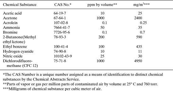
Limitations on occupational exposures to chemicals are set by the Occupational Safety and Health Administration (OSHA), a division of the U.S. Department of Labor. The limitations, often called OSHA Permissible Exposure Limits or OSHA PELs, are listed in Title 29, Part 1910.1000 of the Code of Federal Regulations. Listed in Table 6.2-1 are limitations for air contaminants set by OSHA for representative chemical substances. The relative toxicity of a chemical substance can be gauged by comparing the OSHA PEL for a chemical substance with that for a known poison, hydrogen cyanide, or an irritating but generally nontoxic gas, ammonia. All limitations given in Table 6.2-1 are expressed as time-weighted averages for the chemical substance in any 8-hour work shift of a forty-hour work week. For PELs the action level is not the actual PEL but one-half the PEL, meaning action must be taken at this level to reduce the emissions. An overexposure is observed when monitoring demonstrates an average concentration of a chemical in the workplace greater than the occupational exposure limit over the appropriate time period.
Table 6.2-1 OSHA Permissible Exposure Limits for Air Contaminants.
Control and elimination of unacceptable exposures require information on the source, pathway, and worker exposed to the chemical substance. Control measures can be applied at any step; e.g., process changes can reduce the amount of emissions from various sources. Adjustments in ventilation systems can intercept chemical contaminants and eliminate the pathway for exposure. Finally, personal protective equipment can provide additional protection when other measures are inadequate.
6.2.1 Characterization of the Workplace
The first step in an occupational exposure assessment is to characterize the work-place. Description of the workplace begins with a schematic or written description of the chemical manufacturing process and identification of unit operations where exposure to chemicals may occur. The schematic diagram is used to highlight unit operations and activities where exposure to chemicals may occur, provide a description of production activities and process chemistry, and identify ventilation and other mechanisms that reduce worker exposures. Written descriptions should also include releases and exposures that do not take place in the chemical manufacturing facility, such as transportation and disposal of empty shipping containers.
From an occupational exposure viewpoint, the key elements of a process flow diagram are the sources of potential exposure. A source of potential exposure is a unit operation or worker task that brings the worker into potential contact with the chemical substance. For this reason, sampling points and transfer operations must be highlighted in the schematic diagram or description. Likewise, transfers of materials entering or leaving the process should be described (bagging, drumming, tank truck filling, etc.) since this highlights handling problems that could result in exposure to chemical substances. Waste streams leaving the process should be identified to indicate possible sources of exposure and to provide a resource for environmental studies. The completed flow diagram should highlight possible sources of exposure and minimize the possibility that potential hazards will be overlooked.
The written description should explain the activities occurring in the work area and should emphasize locations where potential exposure to chemicals may occur. It should also include important details such as component stream concentrations, operating temperatures, and pressures. Other factors that affect the potential for exposure (ventilation systems, open-top or closed vessels, use of protective equipment) should be noted in the description. If respiratory or dermal protection is used to limit exposures, the appropriate protection factor provided by the protective equipment should be listed.
Knowledge of the process and its component operations is needed to assess the likelihood and magnitude of exposure of workers to chemical substances. The frequency and duration of sampling events, the duration of batch processes, the type and frequency of transfer operations, and the number of workers involved in each operation are needed to make quantitative estimates of exposures to chemical substances. For convenience, the workers may be separated into groups performing similar operations and thus having similar exposures. A detailed description of the time engaged in each work task (sampling, monitoring unit operations, transferring raw materials and products) and in each work area should be developed where the potential for significant exposure exists.
The schematic and written descriptions can be used to prepare a relatively complete inventory of the chemicals that may be encountered in the work environment and the rates of use or generation of each chemical. For each chemical of concern, the engineer can assemble physical property data (boiling point, vapor pressure, particle size distribution, etc.) which will be of assistance in assessing the potential for exposure. For solid particles, knowledge of the particle size distribution will enable the engineer to evaluate the fraction of airborne particles that are potentially respirable. An excellent source of information on the health effects (nuisance, irritant, toxicity, carcinogenicity, potential for birth defects, etc.) of chemical substances is the Material Safety Data Sheet (MSDS) prepared for each chemical substance by the manufacturer. The MSDS will also provide occupational exposure guidelines established by regulatory or consensus organizations. These include the OSHA PELs, the American Conference of Governmental Industrial Hygienists’ Threshold Limit Values (TLVs), and the American Indus-trial Hygiene Association’s Workplace Environmental Exposure Level (WEEL) guides. OSHA PELs and TLVs are discussed in more detail in Chapter 8 of this text.
6.2.2 Exposure Pathways
Because exposure to chemicals in the work environment can occur through inhalation, skin absorption, or ingestion, the engineer must be aware of these potential pathways into the body. The exposure pathway model in Figure 6.2-1 highlights potential pathways leading from process to worker and provides a framework for evaluating pathways for exposure to chemicals in the workplace. Used in conjunction with the schematic diagram, process description, and physical properties of the chemical substance, the important exposure pathways and controls to minimize exposure can be identified.
Inhalation exposure is often the most significant route of workplace exposure. Chemicals can volatilize from the process or evaporate from work surfaces where they are deposited. Exposure to a high vapor pressure solvent can be evaluated solely from the rate of vaporization and the effectiveness of ventilation controls unless there is also significant skin contact with liquid or vapor. With lower vapor pressure chemicals, longer term volatilization of spills from work surfaces may be important. Dusty environments created by the generation of fine particles, like carbon dust, or in the cleaning of a manufacturing line can also contribute to inhalation exposure.
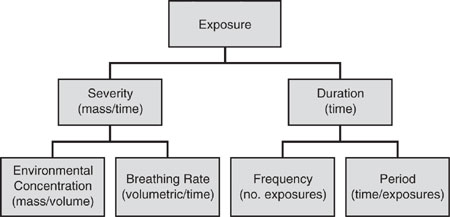
Figure 6.2-2 presents the framework for calculating exposure to chemical substances by the inhalation route. Exposure with units of mass is the product of the severity (mass/time) of exposure and the duration (time) of exposure. Severity is, in turn, the product of the environmental concentration (mass/volume) and the breathing rate (volume/time). Similarly, duration is the product of the frequency (number of exposures) and period (time/exposure) of exposure. A separate esti-mate of the rate of absorption of inhaled materials is necessary to calculate the in-take of a chemical into the body.
Figure 6.2-1 Exposure pathway model.
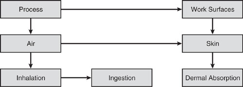
Figure 6.2-2 Inhalation exposure framework.
Dermal contact can also represent an important route of exposure for some chemicals, particularly those that readily absorb through the skin in immediately toxic amounts and those that pass through the skin and accumulate in the body. This exposure pathway usually results from direct contact of chemicals with the skin. Exposure may also result from contact with work surfaces that are contaminated.
Figure 6.2-3 Dermal exposure framework.
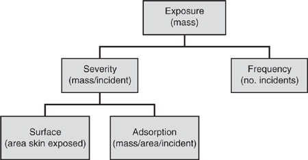
Figure 6.2-3 presents the framework for calculating exposure to chemical substances by the dermal route. Exposure (mass) is the product of severity (mass adsorbed per incident) and frequency (number of incidents). Severity of dermal exposure is, in turn, the product of the surface area of exposed skin and the mass adsorption per incident. Dermal intake into the body requires a separate estimate of the rate of uptake of the chemical from the exposed skin surface.
Oral ingestion of chemicals is usually a relatively minor route of exposure in the workplace, particularly when dining areas are separate from work areas and employees practice a reasonable level of personal hygiene. However, this may be an important route of exposure for chemicals that accumulate in the body over long periods of exposure.
6.2.3 Monitoring Worker Exposure
Monitoring objectives can be grouped into three categories: baseline, diagnostic, and compliance. Baseline monitoring is performed to evaluate the range of worker exposures. The baseline data are used to determine the acceptability of exposures to chemicals and the need for controls to reduce exposures. Diagnostic monitoring is performed to identify principal sources and tasks contributing to exposure to specific chemicals. The results of diagnostic monitoring are used to select appropriate control strategies for reducing exposure to known sources. Compliance monitoring is performed to demonstrate conformance with government regulations. The sampling strategy for evaluating compliance is often to monitor the “most exposed” worker using a collection device attached to the worker near his breathing zone.
Monitoring methods can be classified as either personal monitoring or area monitoring. Personal monitoring is conducted to characterize the exposure of a worker to the chemical substance of interest. The most common method of personal monitoring is a breathing zone measurement. A battery-powered pump is attached to the worker to draw air through a collection tube at a constant rate. The inlet to the collection tube is connected to a flexible hose, which draws air from the breathing zone of the worker. The sample is collected for a designated period and the monitoring result is reported as a time-weighted average over the designated period. Two common sample averaging times are 8 hours, a normal work shift, and 15 minutes, a common short-term exposure time limit. These durations correspond to the averaging times of regulatory limits. Eight-hour sampling has the disadvantage that peak exposure information is usually lost. A mixture of full-shift and short-term sampling is usually the best technique for evaluating worker exposures.
Personal monitoring of skin absorption is often difficult. Patch testing is conducted by affixing a patch of absorbent material to an exposed skin surface of a worker for a known period of time. At the end of a specified time period, the patch is removed and the chemical of concern is extracted from the patch and quantified. Skin washes are used to remove the chemical of concern from the skin surface using a suitable solvent. The quantity of chemical removed from a measured skin area is then quantified and reported as exposure per unit area.
Area monitoring of the ambient air is used to measure the background level of chemical contaminants when chronic conditions resulting from long-term exposure are of concern. Area monitoring is also used to warn of toxic concentrations of acutely hazardous substances. Monitoring the ambient atmosphere can also be used to demonstrate the effectiveness of ventilation controls by measuring the levels of chemical contaminants before and after the controls are installed.
Area monitoring also includes investigation of surface contamination by wipe test methods. Although not a direct method of exposure, wipe tests are useful for tracking levels of contamination, particularly for chemical substances readily absorbed by the dermal route. Wipe tests may be used to document trends in work practices and housekeeping procedures. They can also identify deficiencies in maintenance or operation of local exposure control systems, including safety hoods.
The number of samples collected in a monitoring program is determined by regulatory requirements or professional judgment. The cost and difficulty of sample collection and analysis will limit the number of samples collected. Conversely, a greater number of samples will decrease the likelihood of significant errors in the sample means and decrease the variance about the mean. The standard error of the mean decreases rapidly as the first few replicates are collected but the likely sample error decreases only slightly with each additional sample after 6 to 10 samples are collected. The variance about the sample mean is inversely proportional to the number of samples analyzed. Similarly, the variance about the sample mean decreases significantly over the initial samples and less so after 10 or more samples.
6.2.4 Modeling Inhalation Exposures
It is not always convenient or possible, in the case of a new or proposed process, to undertake a monitoring program to determine airborne concentrations of chemicals. In some instances, a more rapid estimate of potential worker exposures to chemical substances is needed. In this situation, the engineer may utilize models which simulate worker exposures.
6.2.4.1 The Mass Balance Model
A simple model often used to estimate the concentration of airborne contaminants in the workplace is the mass balance model also known as the box model. The work area is modeled as a box in which the contaminant is uniformly distributed. In this case, a mass balance can be written for the contaminant concentration within the work area.
![]()
C is the concentration of airborne contaminant in the work area (mass/length3),
V is the volume of the work area (length3),
t is the time during which the contaminant has been emitted,
G is the emission rate of the contaminant to the air (mass/time),
Q is the ventilation rate in the work area (length3/time),
k is a mixing factor to account for incomplete mixing in the work area (unitless)
Co is the concentration of the airborne contaminant entering the work area
(mass/length3).
If the emission rate and ventilation rate are constant, the concentration will reach a steady state and Equation 6-1 becomes:
![]()
At times, emissions are episodic. Consider a work area that initially contains contaminant at concentration Co. At some time, t=0, an emission source, releasing contaminant at rate G, is placed in the work area. In this case, the box model can be used to estimate the rise in concentration of the contaminant in the workplace. Again, assuming that the ventilation rate is constant, Equation 6-1 can be inte-grated to yield
![]()
The mixing factor (k) typically ranges from 0.3 to 0.7 in small rooms without fans (Drivas 1972). Others have used mixing factors of 0.5 for work areas with average ventilation and 0.1 for poorly ventilated work areas (Fehrenbacher, 1996).
The determination of G may be simple or complex, depending on the nature of the emission source. As an example, assume that the source is a pool of liquid that is evaporating at a constant rate. Estimating this emission rate requires input of the vapor pressure of the contaminant, the surface area of the evaporating liquid, and the relationship between the velocity of the air over the liquid surface and mass transfer from the liquid into the flowing air stream. The penetration model (Hummel et al., 1996) provides acceptable estimates of evaporation rates at low air speeds characteristic of indoor work areas:
![]()
where
G is the evaporation rate (g/sec)
A is the area of the pool/air interface
MW is the molecular weight of the evaporating species (g/mole)
VP is the vapor pressure of the evaporating contaminant (atm)
v is the air velocity parallel to the surface of the evaporating liquid (cm/sec)
T is the surface temperature of the evaporating liquid (oK)
Δ is the length of the evaporating pool in the direction of airflow (cm)
P is the ambient pressure (atm)
A survey and evaluation of other models used to estimate evaporation rates of volatile liquids are given by Lennert (1997).
Example 6.2-1
A cleaning bath for electronic parts emits 0.5 g/sec of CFC-12 into a small work room of dimensions 3 m × 3 m × 2.45 m high. Calculate the concentration in the room under average and poor ventilation conditions if the air velocity in the room is 0.3 m/s and compare the results to the OSHA PEL.
Solution: When the air speed is 0.3 m/s, the volume of air flowing through the room will be:
Q = 0.3 m/s × 3 m × 2.45 m = 2.21 m3/s
and the concentration of CFC-12 in the air will be:
average ventilation C = 0.5 g/sec/(0.5 × 2.21 m3/s = 0.45 g/m3,
poor ventilation C = 0.5 g/sec/(0.1 × 2.21 m3/s = 2.27 g/m3,
A comparison with the permissible exposure limits given in Table 6.2-1 indicates that even under poor ventilation conditions, the OSHA PEL will not be exceeded and respiratory protection will not be needed to safe-guard the health of a person working in this room.
The simple mass-balance model does not account for all of the phenomena that influence the exposure to chemicals released into the workplace atmosphere. Exposure may be mitigated by adsorption of the chemical to walls and other sur-faces in the work room. In this case, the mass balance on the airborne concentration is given by:
![]()
where r is the nonventilatory removal coefficient of airborne contaminant (volume/time). If the ventilation and emission rates are constant, the box model predicts a steady state concentration of:
![]()
Solvents are often volatile and significant accumulations of their vapors may occur in the workplace air. In this instance, the concentration of solvent may exert a significant back pressure retarding the evaporation of additional solvent. Jayjock (1994) has published the solution of the mass balance equation when back pressure is significant.
The approach used in development of the mass-balance model, adjusting the ventilation rate to account for imperfect mixing and unventilated areas, has been criticized because the model is still used to describe an imperfectly mixed room. In addition, the mixing factor is an empirical adjustment that must be developed by experimental measurements. An alternative model divides the work area into two perfectly-mixed zones, one near the source of an airborne contaminant and the other removed from the source (Nicas, 1996). Mixing in the work area occurs as a result of ventilation between the two zones. The steady-state or upper bound on concentration in the zone of the work area nearest the source is given by:
![]()
where
C is the concentration of the contaminant in the work area near the source
(mass/length3)
G is the rate of vaporization of the contaminant (mass/time)
B is the rate of exchange of air between the zones located near and removed from the source (length3/time)
Q is the ventilation rate of the zone removed from the source (length3/time)
Although this model does not require estimation of an empirical mixing factor, the air exchange rate, B, must be determined from the physical dimensions of the zones or other criteria.
Example 6.2-2
Calculate the concentration of freon in the cube, 1 m on a side, surrounding the top of the cleaning bath in Example 6.2-1 if the air exchange rate with the remainder of the room is 1 m3/s. Repeat the calculation for an air exchange rate of 0.5 m3/s.
Solution: From Example 6.2-1, the rate of release of freon from the cleaning unit is 0.5 g/s and the ventilation rate in the room is 2.21 m3/s. Thus in the area closest to the cleaning bath, the concentration of freon can be calculated from Equation 6-7:
C = (0.5 g/s) × [1 m3/s + 2.21 m3/s] / [1 m3/s × 2.21 m3/s] = 0.73 g/m3 = 730 mg/m3
or
c = (0.5 g/s) × [0.5 m3/s + 2.21 m3/s] / [0.5 m3/s × 2.21 m3/s] = 1.23 g/m3 = 1,230 mg/m3
As would be expected, the local concentration of the chemical increases when the ventilation is less. Localized ventilation is an effective method of dispersing airborne chemicals and reducing exposures of workers to chemicals.
6.2.4.2 Dispersion Models
Diffusion of contaminants in workplace air results in the net movement of the contaminants from regions of higher concentration to regions of lower concentration. The spread of the contaminant is aided by the convective mass transfer driven by the ventilation system. The combination of these influences results in movement of contaminants away from their source into the surrounding room (Scheff et al., 1992).
The mass-balance model described above presumes a uniform concentration of the chemical contaminant in the work area. Dispersion models have a notable advantage; they describe the variation of contaminant concentration with distance from the source. The concentration gradient is described by the following equation when convection occurs in the x-direction only and dispersion occurs equally in all directions:
![]()
where
u is the wind velocity in the x direction (length/time)
C is the concentration of airborne contaminant (mass/length3)
D is the diffusion coefficient (length2/time)
x is the distance downwind from the source (length)
r is the distance from the source to the sampling point (length)
This equation has been solved for concentrations resulting from emissions into an infinite space:
![]()
where G is the contaminant emission rate from the source (mass/time).
The diffusion coefficient (D) can be derived from measurements at the sampling site or estimated from values available in the literature. Measurements of the diffusion coefficient in indoor industrial environments have ranged from 0.05 to 11.5 m2/minute, with 0.2 m2/min being a typical value (Jayjock, 1998).
Example 6.2-3
Freon is emitted from an open-top vapor degreaser at a rate of 0.74 g/min. Estimate the concentration in the air inhaled by a worker 3 m downwind from the degreaser if the air velocity is 0.79 m/min.
Solution: Since the worker is downwind of the degreaser, x = r in the diffusion-convection equation and
![]()
Molecular diffusion theory strictly applies to vapors and gases; however, particulate matter with aerodynamic diameters less than 10 μm are distributed in workplace air in a similar manner. Using the dispersion models to describe the distribution of dusts and fumes is reasonable for small particles.
6.2.5 Assessing Dermal Exposures
Dermal hazards refer to chemicals that can cause dermatitis or otherwise damage the skin as well as to chemicals that can enter the body through the skin and cause toxic effects in other organs. Dermatitis refers to inflammation or damage to the skin which is localized and does not spread to other areas of the body. Acids, alkalis, and other irritating or corrosive chemicals damage skin which they contact. Repeated contact with epoxy resins may result in skin sensitization and dermatitis. The National Institute of Occupational Safety and Health has recognized allergic and irritant dermatitis as the second most common occupational disease (after hearing loss), accounting for 15 to 20 percent of all reported occupational diseases. Because of the often readily apparent reaction to chemicals causing dermatitis, exposures are usually quickly eliminated or protective clothing is used to preclude skin contact with toxic chemicals.
In contrast to contact dermatitis, toxic chemicals may be absorbed through the skin, mucous membranes, or eyes either by direct skin contact with the chemical or deposition of aerosols. This absorption can contribute to toxic effects on other organs. Some substances, such as amines and nitriles, pass through the skin so rapidly that the rate at which they enter the body is similar to rates of inhalation or ingestion. In 29 CFR 1910.1000, OSHA identifies nearly 100 chemicals which can enter the body through the skin and cause toxic effects elsewhere within the body. For these chemicals, the engineer should be alert to dermal exposures and should minimize contact of chemicals with the skin by process modifications or use of protective clothing.
The three mechanisms of dermal exposure are 1) direct contact between the worker’s skin and a liquid or solid chemical as from splashing or immersion, 2) transfer of a chemical from a contaminated surface to the skin following direct contact, or 3) deposition or impaction on the skin as a vapor or aerosol. Aerosols are created when chemicals are applied by spraying or when fluids contact moving surfaces, e.g., metal working fluids interacting with machinery. Aerosols tend to settle rapidly, making an increased separation between the worker and operations using the chemical of concern a feasible means of controlling dermal exposures.
The amount of a chemical remaining on the skin depends on the processes of contamination, removal, and penetration through the skin. Possible removal processes are evaporation, incidental transfer to other surfaces, or intentional de-contamination. Dermal exposure is often highly variable between workers over time and between different anatomical locations of the body. Since dermal penetration varies across the anatomical locations of the body, an overall average value for skin exposure is often insufficient.
Direct methods for measurement of skin exposure include collection of chemical contaminants on absorbent pads or clothing and wipe sampling of contaminated surfaces. The absorbent pad technique utilizes gauze pads, treated cloth, or alphacellulose pads which are attached to various sites on the worker’s skin or outer clothing to capture chemicals that would have been deposited on the skin or clothing.
Table 6.2-2 Surface Area by Region of the Body for Adults in Square Centimeters.
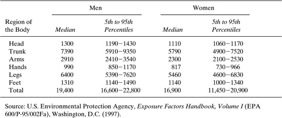
Collection pads are exposed for a representative period of time to the work environment and are subsequently removed and analyzed for the chemical of concern. An estimate of the potential dermal exposure can be obtained by multiplying the amount of contaminant deposited on a unit area of the absorbent pad by the surface area of the body region that the pad is positioned to represent. Data on the surface area of the adult body is given in Table 6.2-2. This technique is generally used for sampling nonvolatile contaminants or compounds with low vapor pressure; charcoalimpregnated cloth has been used for sampling of volatile compounds.
Wipe samples are collected by washing the skin or clothing with water, surfactants, alcohol, acetone, or other solvents. Chemicals remaining on the skin or clothing are collected but those that have penetrated the skin are not collected by this technique. Wipe samples have been used to determine routes of dermal exposure to aromatic amines used as anti-oxidants, intermediates, and curatives in epoxy resins and urethanes. Wipe samples taken from the inside of protective gloves indicated that methylene dianiline used in aircraft composites had penetrated the gloves of workers engaged in the hand lay-up operations in aircraft and aerospace industries. The wipe samples revealed that chemical breakthrough of the protective clothing was the cause of elevated levels of the aromatic amine detected by biological monitoring (Groth, 1992). Wipe tests have also been used to identify significant exposure to toxic chemicals from handling contaminated tools (Klingner, 1992) and improper removal of contaminated clothing (Kusters, 1992).
Computerized image analysis techniques can be used together with fluorescent whitening agents to indirectly quantify exposure of the total body surface (Fenske 1997). Visual observation of fluorescent tracer deposition on skin has been used to characterize exposure in a variety of pesticide applications. The behavior of the fluorescent tracer in the application process must be similar to that of the chemical of concern. This technique provides a means of assessing exposures without use of toxic chemicals.
Methods to control dermal exposure to chemicals can take many forms. Substitution of a less toxic chemical is almost always a good option, unless the alternative chemical has a much higher vapor pressure and is likely to cause an inhalation hazard. Consideration should also be given to redesigning the work process to avoid splashes or immersion. Where that is not feasible, personal protection in the form of chemical protective gloves, an apron, or clothing may be selected. Performance characteristics of glove materials must be matched to the hazard to be avoided, i.e., cuts, abrasions, and dermal contact with toxic chemicals. Glove manufacturers can provide information on the ability of a variety of glove materials (natural rubber, polyvinyl chloride, neoprene, nitrile, butyl rubber, polyvinyl alcohol, viton, or norfoil) to preclude penetration of toxic chemicals.
The quantity of a chemical contacting the skin during immersion, splashing, application to substrate, attachment of process lines, or weighing and transfer of chemicals can be estimated as the sum of the products of the exposed skin areas (in cm2) and the amount of chemical contacting the exposed area of the skin (mg/cm2/event). Usually, the amount of chemical transferred to the exposed area can only be measured after exposure has occurred. If the chemical of concern is absorbed rapidly, the amount of chemical contacting the skin will be greater than that estimated by direct measurement; indirect methods of measurement of exposure such as the fluorescent imaging described above may be required to obtain accurate estimates of dermal exposure.
During most dermal exposure events, exposure will be limited to a few areas of the body. For example, during sampling of a reactor, attachment of process lines, or manual weighing and dumping of powders, only the hands and perhaps the forearms would be exposed to the chemical of concern. Conversely, during the spray application of a paint, addition of a antimicrobial liquid to latex products, use of metal working fluids, or commercial pesticide applications, concern for aerosols, splashing of fluids, and general dispersion of the chemical will require that other areas of the body be protected from contact with process chemicals.
The equation given below can be used to estimate the exposure to a chemical that is absorbed through the skin.
![]()
where
DA is the dermal absorbed dose rate of the chemical (mass/time)
S is the surface area of the skin contacted by the chemical (length2)
Q is the quantity deposited on the skin per event (mass/length2/event)
N is the number of exposure events per day (event/time)
WF is the weight fraction of the chemical of concern in the mixture (dimensionless)
ABS is the fraction of the applied dose absorbed during the event (dimensionless)
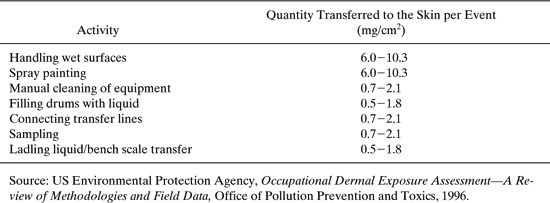
In the absence of monitoring data, the values given in Table 6.2-3 may be used to estimate dermal exposure to liquids during plant operations.
Table 6.2-3 Quantity of Chemical Deposited on the Skin per Exposure Event.
Example 6.2-4
A worker is preparing an epoxy adhesive by adding the solvent (toluene) and the chemicals to produce the adhesive in a batch reactor. During the process, the reactor is sampled twice. At the end of the reaction, the worker fills drums with the epoxy adhesive and cleans the reactor. Estimate the dermal exposure of the worker to toluene. Assume the adhesive contains 20 percent toluene.
Solution: Equation 6-10 and the higher limits of dermal exposure given in Table 6.2-3 will be used to obtain a conservative estimate of dermal exposure. The skin surface areas for the hands are given in Table 6.2-2. Assume all of the toluene contacting the worker’s hands is absorbed, that only one hand is exposed during sampling, and that both hands are exposed during other operations.
Connecting toluene inlet line: (840 cm2) (2.1 mg/cm2/event) (1 event) (1.0) (1.0) = 1,760 mg
Sampling reactor: (420 cm) (2.1 mg/cm/event) (2 events) (1.0) (0.2) = 350 mg
Filling drums with product: (840 cm) (1.8 mg/cm/event) (1 event) (1.0) (0.2) = 300 mg
Cleaning reactor: (840 cm) (2.1 mg/cm/event) (1 event) (1.0) (0.2) = 350 mg
Total potential exposure to toluene: 2,760 mg
Some chemicals will be absorbed through the skin during the exposure event, some will be absorbed after the exposure event, and some chemicals will be removed before absorption occurs. Fick’s first law of diffusion has been used to characterize the rate of penetration of the skin. The skin is resistant to hydrophilic or water-soluble chemicals and the permeability constant is unlikely to exceed 0.001 cm/hr. Hydrophobic compounds are more readily absorbed and the penetration of organic solvents such as toluene and xylene may approach 1 cm/hr (US EPA, 1992). It has been recommended that the time during which absorption occurs be taken as four hours and that the fraction of the chemical remaining on the surface of the skin longer than four hours will be removed (Fehrenbacher, 1998).
Equation 6-11 can be used to estimate the uptake of a chemical that is absorbed through the skin when evaporation and organic solvent carrier effects are negligible.
![]()
where
DA is the dermal absorbed dose of the chemical (mass)
S is the surface area of the skin contacted by the chemical (length2)
Kp is the permeability coefficient for the chemical of concern (length/time)
ED is the exposure duration (time)
WF is the weight fraction of the chemical of concern in the mixture (dimensionless)
ρ is the density of the mixture (mass/length3)
The following equation for the permeability coefficient was selected after independent statistical analysis of data for diffusion of organics in aqueous solution through the skin (US EPA 1992).
![]()
where
Kp is the permeability coefficient of the chemical of concern through the skin (cm/hr)
Kow is the oil-water partition coefficient (dimensionless)
MW is molecular weight of the chemical of concern (mass/mole)
When the chemical of concern is dissolved in an organic solvent, the permeability of the skin to the organic solvent should be used to calculate the dermal absorption rate.
Example 6.2-5
A worker is dying cloth in a 15% by weight aqueous solution of the dye Red No. 19. The worker exposes his hands and forearms to the dye for 8 hours each work day. The density of the mixture is 1,030 kg/m3. Physical properties of Red No. 19 include a Kow of 1.0 and a molecular weight of 479 grams per gram-mole. Calculate the daily dermal uptake of Red No. 19 by the dye worker.
Solution: Equation 6-12 can be used to estimate the permeability coefficient for the dye Red No. 19; subsequently, Equation 6-11 can be used to calculate the absorbed dose. The median surface area of the hands and forearms of an adult male is 0.23 square meters.
log(kp) = -2.72 + 0.71 log (1.0) - 0.0061 (479) = -5.64; Kp = 2.28 × 10⁻⁶ cm/hr
DA = (0.23 m2) (2.28 × 10⁻⁸ m/hr) (8hr/workday) (0.15) (1,030 kg/m3) (106 mg/kg) = 6.5 mg/workday
Section 6.2 Questions For Discussion
1. For what types of chemicals would dermal exposures be more significant than inhalation exposures in the workplace?
2. For what types of processing operations would dermal exposures be more significant than inhalation in the workplace?
3. The simple exposure estimation procedures described in this section are useful primarily as screening tools. If these methods indicate potentially high exposures, more sophisticated models should be employed. Describe some of the chemical and physical processes important to inhalation and dermal exposure that more complex models should address.
6.3 Exposure Assessment For Chemicals in the Ambient Environment
Exposure to chemicals in the ambient environment can occur through inhalation, ingestion, or dermal contact. Typically, exposure by ingestion is not as important as dermal or inhalation exposure. However, ingestion may be a significant route of exposure to chemical substances when animals used for food, such as fish or shell-fish, accumulate and concentrate chemical contaminants. Ingestion may occur when particles are trapped and swallowed following respiration or when small children eat dust or soil. Ordinarily, exposure by inhalation or dermal absorption will accompany ingestion and result in more significant uptake of the chemicals of concern. In this section, only inhalation and dermal exposure will be considered.
Assessment begins with identification of all wastes and releases containing a chemical of concern and an estimate of the quantity of waste disposed from each source. Next, the concentration of the chemical of concern in the waste or release is measured or estimated and the characteristics of the waste matrix, such as whether it is a liquid, gas, or solid, are identified. The treatment and disposal practices associated with each waste are identified and the quantity of the chemical of concern released to the air, surface waters, groundwater, and land by the treatment and disposal practices are estimated. Finally, the transport and transformation of the chemical of concern through the air, surface waters, and ground water is modeled, along with the uptake through inhalation, ingestion, or dermal contact. In this section, exposure assessment is used to determine the amount of a chemical of concern potentially contacting a member of the general population.
6.3.1 Exposure to Toxic Air Pollutants
Exposure assessment for toxic air pollutants is a four-step process. The first step is to identify pollutants likely to be in the ambient air. Many chemicals found in factories, consumer goods, and waste treatment plants can be released to the air as toxic air pollutants. Some commonly released chemicals include perchloroethylene from dry cleaners, methylene chloride from industrial cleaning and consumer products such as paint strippers, and chromium from metal plating operations. The Toxic Release Inventory, available at the EPA website (www.epa.gov) and discussed elsewhere in this text, provides an extensive source of data on toxic chemical releases.
The second step in exposure assessment for toxic air pollutants is to estimate the quantities of pollutants released by point, area, and mobile sources. Point sources are sites with a specific, usually fixed, location. Point sources include chemical plants, steel mills, oil refineries, and hazardous waste incinerators. Pollutants can be released when equipment leaks, when chemicals are transferred from one area to another, or when pollutants are emitted from stacks. Area sources of toxic air pollutants are comprised of many small sources releasing pollutants to the outdoor air in a defined area. Examples include dry cleaners, small metal plating operations, and gas stations. Mobile sources include automobiles, trucks, buses, etc., which are important contributors of oxides of nitrogen and sulfur, hydrocarbons, carbon dioxide, and particulates in the air.
Routine releases, such as those from industry, cars, landfills, or incinerators, may follow regular patterns and occur continuously over time. Other releases may be routine but intermittent, such as when production is done in batches. Accidental releases can occur during an explosion, equipment failure, or a transportation accident; the timing and, often, the amount released during accidental releases are difficult to predict.
To estimate the amount of a routine or intermittent release, engineers will often sample the effluent from a facility as it is released. The sample is taken to a laboratory and analyzed to quantify the amount released during the collection period. The amount collected during the test is used to predict the amount released each operating day. For example, if 0.1 kilogram of sulfur dioxide is collected in one hour by a collector which samples 1 percent of the airflow from a stack, a plant operating 24 hours per day would be expected to emit 240 kg of sulfur dioxide per day.
Alternatively, engineers can use an emission factor to estimate the amount of toxic air pollutant released by a particular facility. Emission factors are averages of emission measurements from a few representative facilities that relate the quantity of a pollutant released to the level of production associated with the release of that pollutant. Emission factors are described in detail in later chapters. Example 6.3-1 illustrates the use of a particularly simple emission factor.
Example 6.3-1 Use of Emission Factors
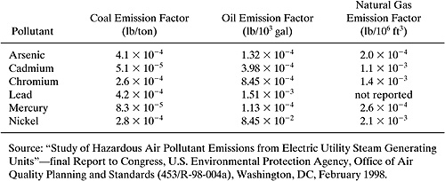
An electrical power generating station with four electrical generating units burned 1,055,539 tons of coal, 22,122 thousand gallons of No. 6 fuel oil, and 606 million cubic feet of natural gas to generate electricity during 1998. Use the emission factors in the table below to estimate the releases of arsenic and mercury from the stacks at the power plant.
Solution:
Arsenic: | (1,055,539 tons)(4.1 × 10⁻⁴ lb/ton) + (22,122 × 103 gal)(1.32 × 10⁻⁴ lb/103 gal) + (606 106 cf)(2.0 × 10⁻⁴ lb/106 cf) = 436 lbs. |
Mercury: | (1,055,539 tons)(8.3 10-5 lb/ton) + (22,122 103 gal)(1.13 × 10⁻⁴ lb/103 gal) + (606 106 cf)(2.6 × 10⁻⁴ lb/106 cf) = 90.3 lbs |
The third step is to estimate the concentration of the toxic pollutant at the location where exposure occurs. The concentration of a pollutant decreases as it disperses from the point of release. The decrease in concentration or dispersion of the toxic air pollutant is a function of the wind direction and speed and the terrain over which the air flows, whether flat or hilly, whether flowing over a mountain or through a valley. The location of the release, whether from a tall smokestack or a leak at ground level, will affect the distribution of the pollutant near the facility; a toxic air contaminant released from high stacks is dispersed and diluted while descending to ground level. Other factors that affect the concentration include the temperature and speed of the gas exiting the smoke stack and the location of the release within the facility.
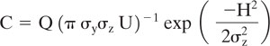
The Gaussian dispersion model is most often used to characterize the dilution of toxic air pollutants with distance from the source. The model provides reasonable agreement with experimental data and is, in its simplest form, easy to perform calculations with. The mean concentration, C, resulting from emission at a continuous point source of strength Q at a height H above the totally reflecting earth along the plume centerline is given by
where
C is the concentration of toxic air pollutant (g/m3)
Q is the source release rate (g/s)
U is the mean wind speed at the stack height (m/s)
H is the effective height of release above the earth (m)
y is the distance in a direction transverse to the wind (m)
z is the height at which the observation is made (m)
σy and σz are the standard deviations of the concentrations of plume transverse to the wind and perpendicular to the earth, respectively (m)
Published values of σy and σz are based on laboratory and field measurements of velocity fluctuations under a variety of atmospheric conditions. Atmospheric stability is used to represent the amount of mixing in the atmosphere and is generally classified as stable, neutral, or unstable. A stable atmosphere is characterized by temperatures that increase with distance from the surface of the earth and reduced vertical mixing; nighttime atmospheric conditions are generally represented as stable. More vigorous atmospheric mixing is expected as the sun warms the surface of the earth and the warmer, less dense air accumulates near the earth’s surface; eventually, gravity will displace the warm air with cooler air from above. Daytime atmospheric conditions are typically represented as either neutral or unstable.
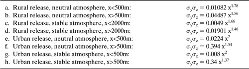
The product of the standard deviations has been represented by an equation of the form
![]()
where
a and b are constants (nondimensional)
x is the distance downwind from the source (length)
Kumar (1998, 1999) performed regression analysis to develop expressions for the constants, a and b, for urban and rural settings and neutral and stable atmospheric conditions. Urban settings are appropriate when there are many obstacles in the immediate area of the release; obstacles include buildings and trees. Rural settings are appropriate when there are no buildings in the immediate area of the release and the terrain is generally flat and unobstructed. Table 6.3-1 lists the results of the regression when the distance from the source is in meters.
Table 6.3-1 Regression Equations for Dispersion Coefficients.
Example 6.3-2
Hydrogen sulfide is released from a low-level vent in a rural area at a rate of 0.025 kg/s. Calculate the concentration at the plant boundary located 300 m downwind from the vent during daytime conditions when the wind speed is 4 m/s and at night when the wind speed is 2.5 m/s. (a) If the concentration of concern for hydrogen sulfide is 42 mg/m3, will this concentration be exceeded at the plant boundary? (b) Estimate the exposure to hydrogen sulfide of a person living 300 m downwind from the facility described during i) daytime and ii) nighttime if the individual at rest breathes 0.9 m3/hr of the ambient air.
(a) Equation 6-13 can be used to calculate the concentration at ground-level by setting the height above the earth equal to zero. The appropriate correlations for the dispersion coefficients are given by items a and c in Table 6.3-1 for daytime and nighttime conditions, respectively. For daytime conditions, For nighttime conditions,
![]()
For nighttime conditions,
![]()
The concentration of hydrogen sulfide is below the concentration of concern under daytime conditions but exceeds the concentration of concern at night when atmospheric mixing is less.
(b) For daytime condition, (7.17 mg/m3) (0.9 m3/hr) 6.45 mg/hr
For nighttime conditions, (50.2 mg/m3) (0.9 m3/hr) 45.2 mg/hr
The last step in an exposure assessment is to estimate the number of persons exposed to a toxic air pollutant. Demographers can estimate the number of persons living in areas surrounding a source using census data. Combining the concentration estimates and the census data, engineers can estimate the numbers of people exposed to the pollutant at varied concentrations. To aid decision makers, these results can be compared to a selected benchmark such as an air quality standard or a level with a known health effect. Data on population densities in regions surrounding point sources are available at the Envirofacts section of the EPA website (http://www.epa.gov/enviro/index_java.html, see Appendix F).
6.3.2 Dermal Exposure to Chemicals in the Ambient Environment
Swimming in rivers, lakes, and streams is generally the only activity considered to cause significant dermal exposure. Although other activities—e.g., water skiing, fishing, standing in the rain—could lead to human dermal exposure, the frequency, duration, and the amount of skin surface available for exposure are small; there-fore, for general and long-term assessments, these activities are considered negligible. Because swimming is an episodic activity, it is necessary to consider both frequency and duration of exposure. In addition, the surface area exposed is an important factor in dermal exposure calculation. These activity-related parameters, when coupled with data on the aquatic ambient concentration of a chemical toxin, yield an estimate of dermal exposure.
Frequency of swimming in natural surface water bodies can be defined from the number and duration of exposures occurring in a single year. A Department of Interior survey (USDOI 1973) found that 34% of the population swam in rivers, lakes, or oceans in the year surveyed. For these swimmers, the average frequency of swimming was seven days per year and the average duration was 2.6 hours. Subsequent investigation of this survey found that the reported exposure time represented time on the shore as well as time in the water (EPA 1992). Furthermore, certain subpopulations, e.g., competitive swimmers, upwardly biased the average exposure frequency and time. Therefore, a reasonable average frequency for a recreational swimmer may be 5 days per year lasting 0.5 hour on each day when swimming occurs (EPA 1992).
An inherent assumption of many exposure scenarios is that clothing prevents dermal contact and subsequent absorption of contaminants. For swimming and bathing scenarios, past exposure assessments have assumed that 75% to 100% of the skin surface is exposed (Vandeven and Herrinton, 1989). Other studies have shown that dermal exposure may occur at sites covered by clothing (Maddy et al., 1983). Consequently, it is appropriate to assume that the entire body is exposed to the chemical of concern during swimming.
Data on the surface area of the body is given in the Exposure Factors Hand-book (EPA 1997) and reproduced in Section 6.2. As shown in Table 6.2-1, total adult body surface area for males can vary from less than 1.7 square meters to over 2.3 m2; for females, the range is from 1.45 m2 to 2.1 m2. For default purposes, the median skin surface areas, 1.94 m2 for males and 1.69 m2 for females, can be used.
Example 6.3-3
A man swims in a river downstream of a rubber processing plant that uses 1,1,1-trichloroethylene to clean molds used to shape the rubber parts. Wastewater dis-charged into the river results in contamination at a level of 3 g per liter in the receiving stream. The man is of average stature and swims in the river about fifteen times each summer with each swim lasting one-half hour. Calculate the man’s exposure to 1,1,1-trichloroethylene which results from swimming in the river.
Solution:
Exposure = (Mass/Event)*(15 events/yr)
Mass/Event is obtained from Equations 6-11 and 6-12 where
s 1.94 m2
Kp 10-1.8 cm/hr
ED 0.5 hr
WF 3μg trichloroethylene per 1000g H2O
ρ = 106 g/m3
Exposure 5 ×10⁻⁷ (g TCE/event) (15 events/yr) 7.5 ×10⁻⁶ (g TCE/yr)
6.3.3 Effect of Chemical Releases to Surface Waters on Aquatic Biota
Wastewater generated in the manufacture, processing, or use of a chemical may contain a fraction of the chemical produced and the raw materials used in the manufacturing process. This loss may occur during reaction to produce the chemical, purification, blending, or cleaning of the reactors, piping, and equipment used to process the chemical substance. The wastewater must be either treated by facilities at the plant site or, more often, commingled with the wastes of others and treated at a publicly owned treatment works (POTW). Using physical-chemical property data and estimates of biodegradability, the effectiveness of the treatment can be estimated, so that the amount actually entering the receiving water body can be predicted. The receiving water body will dilute the discharge from the plant site or POTW so that the concentration in the receiving stream can be calculated if the flow in the stream is known. Stream in this context means the receiving body of water and, in this sense, can include creeks, rivers, lakes, bays, or estuaries.
Removal of chemicals during wastewater treatment is controlled by the physical and biological processes employed in the treatment works. The following processes are commonly used to remove chemicals during wastewater treatment:
1. Adsorption to suspended solids in the primary clarifier, aeration basin, and secondary clarifier;
2. Volatilization through surface vaporization in the primary and secondary clarifiers and through air-stripping in the aeration basin; and
3. Biodegradation by aerobic microorganisms, most commonly in an activated sludge aeration basin.
Under optimal conditions, a POTW will remove a large percentage, i.e., 70 to 99 %, of many organic pollutants from the wastewater, but treatment efficiency varies with the chemical and physical properties of the pollutant. The POTW is typically less efficient in removal of inorganic pollutants and many of these pass through the POTW unchanged.
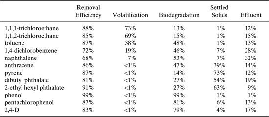
Numerous models have been proposed to predict the fate of chemicals in a POTW consisting of a primary settling basin, an activated-sludge aeration basin, and a secondary clarifier. Clark, et al. (1995) proposed a simple fugacity analysis of the fate of organic chemicals in a POTW. The fugacity approach is predicated on equivalence of the chemical potential in phases in contact, in this case wastewater, solids suspended in the wastewater, and air in contact with the wastewater. The physical-chemical properties needed to model the fate of chemicals in a POTW by the fugacity analysis include water solubility, vapor pressure, octanol-water partition coefficient, and biodegradation half-life. These properties are discussed in Chapter 5 of this text. Sample removal efficiencies as calculated by Clark, et al. (1995) are shown in Table 6.3-2.
An important issue for surface water is the effect that a chemical may have on aquatic organisms including algae, freshwater crustaceans, and fish. A healthy stream with a wider variety of organisms will have a better ability to assimilate chemical releases than a stream whose quality is already compromised. If any link in the food chain in a stream is impacted, the effect can be deleterious to other organisms as well as the health of the stream. Organisms lower on the food chain, such as algae, have shorter lives; for these organisms short-term exposures to high concentrations of chemicals are critical. Consequently, the concentration of a chemical in the receiving body of water when the dilution is least is used to assess the impact of chemical releases on the aquatic biota. For this purpose, the historical stream flow representing the seven consecutive days of lowest flow over a ten-year period is often used to generate estimates of chronic concentrations of chemicals of concern for aquatic life. Data on historical stream flows is available from the U.S. Geological Survey or at the agency’s Internet site at http://www.usgs.gov/usa/nwis/sw.
Table 6.3-2 Removal Efficiencies in a POTW Calculated by Clark, et al. (1995).
The following formula can be used to calculate surface water concentrations of the chemical of concern in free-flowing rivers and streams:
SWC = [Release × (1 – WWT/100)]/Stream flow] (Eq. 6-15)
where
SWC is the surface water concentration (mass/volume)
Release is the quantity of chemical released in wastewater (mass/time)
WWT is the percent removal in wastewater treatment (dimensionless)
Stream flow is the measured or estimated flow of the receiving stream (volume/time)
Example 6.3-4
During periodic cleaning of reactors, a chemical plant using toluene as a process sol-vent discharges wastewater containing 32 kg/day of toluene to the Riverside POTW. The Riverside facility is an activated sludge plant with primary and secondary treatment for wastewater pollutants. The Riverside plant discharges its effluent into the Grande River which has a historical once-in-ten-years 7-day low-flow of 84 cfs. Assess the potential impact of the discharge on minnows in the river if the LC-50 for the minnows is 20 mg/l.
Solution: Using the estimated removal efficiency for toluene from Table 6.3-2 of 87%, the estimated concentration of toluene in the Grande River at low-flow conditions can be calculated using Equation 6-15.
![]()
The estimated concentration of toluene is three orders of magnitude (1000 times) less than that which would be lethal to one-half of the minnows. This is a reasonable margin of safety for aquatic biota.
6.3.4 Ground Water Contamination
Industrial solid wastes are often sent to land disposal in municipal, industrial, or hazardous waste landfills. Although less common, surface impoundments and land treatment may be used to contain and treat industrial wastes. Chemicals may leach from the wastes, either in free liquid contained in the waste or in rainwater percolating through the waste, and be carried into the underlying soils. Chemicals entering the soil solubilize in water contained in the pore space between the soil particles. This interstitial water, called groundwater, may subsequently percolate downward into the water table, carrying the chemical contaminants with it.
Groundwater contamination is most common beneath urban areas, agricultural areas, and industrial complexes. Frequently, groundwater contamination is not discovered until long after the actions leading to the contamination have occurred. One reason for this is the slow movement of groundwater through soils and underlying rock strata; in fine-grained soils and low permeability rock strata, groundwater movement is often less than one foot per day. Contaminants in groundwater do not mix or spread quickly, but remain concentrated in slow-moving, localized plumes that may persist for many years. This often results in a delay in the detection of groundwater contamination. In some cases, groundwater contamination discovered today is the result of agricultural, industrial, and municipal practices several decades ago. This also means that the land disposal practices of today may have effects on groundwater quality many years from now.
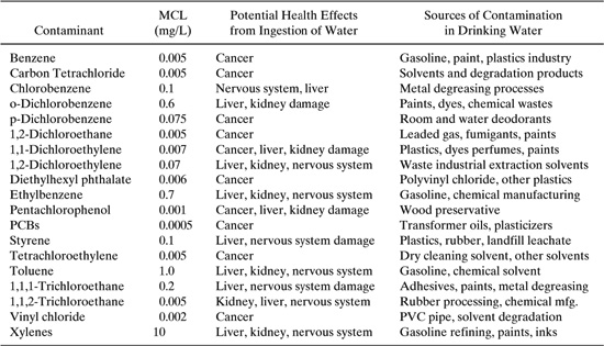
Groundwater is a vital natural resource. It is used for public and domestic water supply, for irrigation of crops, and for industrial, commercial, mining, and thermoelectric power production purposes. In 1990, the United States Geological Survey reported that groundwater supplied 51% of the nation’s total population with drinking water. Unfortunately, groundwater is vulnerable to contamination and, once contaminated, is difficult to remediate. Table 6.3-3 lists National Primary Drinking Water Standards prescribed by the US Environmental Protection Agency which must be met by all drinking water supplies after treatment, if any.
The transport of a chemical in the subsurface depends on physical-chemical properties of the chemical and the characteristics of the subsurface environment. Some of the more important properties influencing the spread of chemical contaminants in the subsurface include water solubility, soil organic carbon partition coefficient, and vapor pressure. A chemical that is readily soluble in water will be carried deeper into the subsurface by rainwater and once it reaches the water table it will mix intimately with the groundwater. A chemical that has an affinity for organic solvents is likely to be adsorbed onto soil organic matter which constitutes a range of less than 1% to 20% of topsoils with the concentration generally decreasing with increasing depth; adsorption from the groundwater retards the movement of dissolved chemicals. In addition, cationic species can be expected to attach to soil particles that are negatively charged. Chemicals with significant vapor pressure may vaporize to the atmosphere from shallow pore water before precipitation carries the chemical downward to the saturated zone.
Table 6.3-3 National Primary Drinking Water Standards for Maximum Contaminant Limits (MCL), US EPA 1994.
Even the simplest descriptions of contaminant migration in groundwater often rely on numerical solutions of the equations governing flow, physical equilibrium, and chemical reaction. Analytical solutions are available for a variety of conditions when only a single spatial dimension is considered (van Genuchten and Alves, 1982). For example, the one-dimensional form of the analytical equation for convection and dispersion for dissolved, nonreactive constituents in a homogeneous sediment is
![]()
where
C is the concentration of dissolved solute in the groundwater (mass/volume)
D is the hydrodynamic dispersivity in the direction of flow (length2/time)
u is the average interstitial groundwater velocity (length/time)
x is the distance along the flow path (length)
t is the temporal variable (time)
Hydrodynamic dispersion is due to mixing of the groundwater and molecular diffusion of the dissolved species. These components are combined to yield
where
σ is the dynamic dispersivity of the porous media (length, typical value for is 0.1)
D* is the coefficient of molecular diffusion of the solute (length2/time)
The boundary conditions for a step function input are described mathematically as
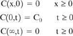
For these boundary conditions, the solution to Equation 6-16 for a saturated, homogeneous porous media is given by
![]()
where erfc is the complementary error function, which is tabulated in mathematical handbooks.
One-dimensional expressions for the transport of dissolved constituents, such as Equation 6-18, are of limited utility in field problems because dispersion occurs in directions transverse to flow as well as in the direction of flow. Baetsle (1969) has described the concentration distribution in a plume of contamination originating as an instantaneous slug at the point x 0, y 0, z 0. As the contamination is carried away from the source in the x-direction, the concentration distribution resulting from instantaneous release of a mass M is given by
![]()
The maximum concentration in the plume occurs at the center of mass of the contaminant cloud where x ut, y 0, z 0, at which the exponential term is equal to unity. The zone in which 99.7% of the contaminant mass occurs is described by the ellipsoid with dimensions, measured from the center of mass, of di (2Dit)1/2 where i x, y, or z.
Example 6.3-5
A rupture of a storage tank containing liquid waste released 100 kg of dissolved arsenic into a shallow saturated groundwater zone in which the flow is horizontal. The average groundwater velocity is 0.5 m/day, the dynamic dispersivity is 0.1 m, and the coefficient of molecular diffusion of arsenic in water is 2 10-8 m2/s. Arsenic is not removed from the groundwater by adsorption or chemical precipitation. Estimate the location and size of the waste plume 90 days after the rupture of the tank.
Solution: After 90 days, the center of gravity of the contaminant plume has moved (0.5 m/day)(90 days) 45 meters from the site of the rupture in the direction of groundwater flow. The dispersivities in the coordinate directions are, in the absence of better data, estimated to be:
Dx = (0.1 m)(0.5 m/day) + (2 × 10⁻⁸ m2/s)(86,400s/day) = 0.0517 m2/day
Dy = Dz = (2 × 10⁻⁸m2/s)(86,400 s/day) = 1.73 × 10⁻³m2/day
The extension of the plume from the center of gravity in the three dimensions are
dx = [(2)(0.0517 m2/day)(90 days)]1/2 = 3.05 m ahead and behind the center of the plume
dy = dz = [(2)(1.73 × 10⁻³ m2/day(90 days)]1/2 = 0.56 m above, below, and to either side
The concentration at the center of the plume is
![]()
Section 6.3 Questions for Discussion
1. What classes of chemicals will be highly mobile in groundwater and what classes of chemicals would be relatively immobile?
2. What classes of chemicals will be likely to be present at high concentrations in sur-face waters, even after treatment in POTWs and other wastewater treatment units?
3. The simple exposure estimation procedures described in this section are useful primarily as screening tools. If these methods indicate potentially high exposures, more sophisticated models should be employed. Describe some of the chemical and physical processes important to determining concentrations of contaminants in surface and groundwaters.
6.4 Designing Safer Chemicals
A challenge for chemical engineers is to use the general principles outlined in this chapter and in Chapter 5 in designing chemicals that will reduce toxicity. The remainder of this chapter presents semi-quantitative principles and guidelines that can be used in designing safer chemicals and is adapted from material presented by DeVito (1996).
In designing safer chemicals, it is useful to think about modifying properties so that
• persistence and dispersion in the environment are minimized, reducing exposures,
• uptake by the body is minimized, reducing dose, and
• toxicity is minimized.
This section will consider property modifications that can lead to reduced exposure, dose, and toxicity. Consider first the issue of dose.
6.4.1 Reducing Dose
Converting an exposure (e.g., inhaling a chemical) into a dose (e.g., absorption by the blood through the lung membrane) generally involves the transport of a chemical across a membrane. The three primary membranes of interest are the lung, which controls uptake of chemicals that are inhaled; the skin, which controls the uptake of compounds from dermal exposures; and the gastrointestinal tract, which controls the uptake of chemicals that are ingested. Some of the characteristics of these membranes are listed in Table 6.4-1.
From Table 6.4-1, it is apparent that the gastrointestinal tract has one of the greatest surface areas available for uptake of chemicals by the body. The uptake of chemicals across this membrane is controlled by lipid solubility, water solubility, dissociation constant, and molecular size.
High water solubility enhances uptake through the gastrointestinal tract because water soluble materials are more easily mobilized in the large and small intestine and the materials therefore experience less mass transfer resistance in migrating to the intestine wall. In contrast, high lipid solubility enhances uptake and transport across the membrane. Thus, the compounds that are likely to be transported from the gastrointestinal tract into the blood streams are compounds with moderate water solubility and moderate lipid solubility. Highly water soluble (lipid insoluble) and highly lipid soluble (log Kow > 5, water insoluble) compounds are less likely to be taken up through the gastrointestinal tract.
Molecular weight also plays a role in determining uptake through the gastrointestinal tract. A general guideline is that molecules with molecular weights less than 300 that are both lipid and water soluble are well absorbed, and those with molecular weights in excess of 1000 are only sparingly absorbed.
The lung also provides a relatively large surface area for uptake of chemicals. The lung is a relatively thin membrane and because the membrane is so thin, lipid solubility plays less of a role in chemical uptake than for the gastrointestinal tract. High water solubility will promote uptake through the lung, as will the delivery of the compound on fine particles (less than 1 micron in diameter). Small particles can be inhaled deeply and will deposit deep in the lung, allowing the chemicals adsorbed on or dissolved in the particles to reside in the lung for very long periods.
The skin presents a formidable barrier to chemicals transport. For a chemical to be taken up through the skin, it must pass through multiple layers. As with the gastrointestinal tract, moderate lipophilicity (log Kow < 5) promotes absorption through the skin because transport must occur through both largely lipid and largely aqueous layers.
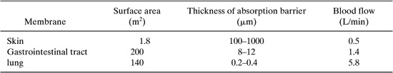
Table 6.4-1 Characteristics of Membranes That Control Chemical Uptake by the Body (DeVito, 1996).
Finally, note that once a compound is absorbed into the blood stream, it must still reach a target organ. Many organs have their own barriers to uptake that may influence dose (e.g., the blood-brain barrier is more easily crossed by lipophilic materials). In addition, chemicals may be removed by the body through urine and feces before the target organ is reached (water solubility enhances elimination via this mechanism).
6.4.2 Reducing Toxicity
Designing safer chemicals by reducing toxicity requires a knowledge of the mechanisms by which compounds exert a toxic effect. While these mechanisms are not known in many cases, there are a few general mechanisms for toxicity that can be examined, leading to safer chemical designs.
One group of mechanisms associated with toxic effects are the reactions of electrophilic species with nucleophilic substituents of cellular macromolecules such as DNA, RNA, enzymes and proteins. Table 6.4-2 presents the possible effects of a number of common electrophiles.
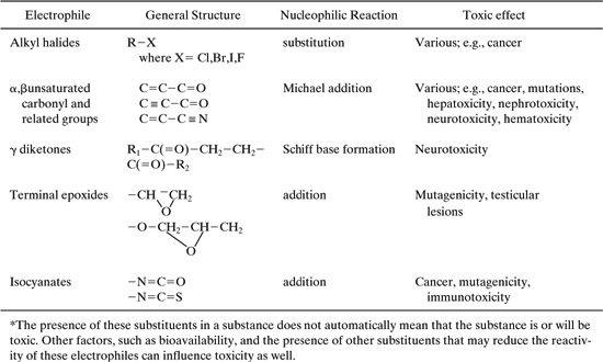
Table 6.4-2 Examples of Electrophilic Substituents and the Reactions They Undergo with Biological Nucleophiles, and the Resulting Toxicity* (DeVito, 1996).
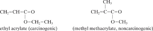
Ideally, the use of these groups would be avoided, however, in many cases the electrophilic groups are necessary to produce a desired property. For example, for the case of the unsaturated carbonyls, the Michael addition reaction that causes the toxic effect may be the desired commercial property. Nevertheless, the toxic effects can sometimes be reduced by introducing selected substituents. For example, the addition of a methyl substituent to ethyl acrylate reduces potential health effects:
Isocyanates present another example. In this case, the electrophilic nature of the isocyanate can be masked in some applications by converting the material to a ketoxime derivative.
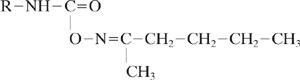
The ketoxime derivative is then removed, in situ, during the use of the compound. This reduces potential exposures and the resultant toxicity.
Clearly, the identification of such structural modifications requires a detailed knowledge of the mechanism of the potential toxicity and the structural sensitivity of that mechanism. Case studies of structural modifications leading to reduced toxicities are available in the US EPA’s Green Chemistry Expert System, which is available at http://www.epa.gov/greenchemistry/gces.htm. Such detailed knowledge is not available for all materials, but the examples cited above demonstrate that there is potential for designing materials with reduced toxicities.
References
Baetsle, L.H., “Migration of radionuclides in porous media,” Progress in Nuclear Energy, Series XII, Health Physics, A.M.F. Duhamel, ed., Pergamon Press, Elmsford, N.Y. (1969).
Clark, B., Henry, J.G., and Mackay, D., “Fugacity analysis and model of organic chemical fate in a sewage treatment plant,” Environ. Sci. Technol., 29, 1488–1494 (1995).
DeVito, S., “General Principles for the Design of Safer Chemicals: Toxicological Considerations for Chemists,” Designing Safer Chemicals, American Chemical Society, Symposium Series 640, Washington, D.C., 1996.
Drivas, P.J., Simmonds, P.G., and Shair, F.H., “Experimental characterization of ventilation systems in buildings,” Environ. Sci. & Tech., 6, 609–614 (1972).
Fenske, R.A., and Birnbaum, S.G., “Second generation video imaging technique for assessing dermal exposure (VITAE system),” Am. Ind. Hyg. Assoc. J., 58, 636–645 (1997).
Fehrenbacher, M.C. and Hummel, A.A., “Evaluation of the mass balance model used by the Environmental Protection Agency for estimating inhalation exposure to new chemical substances” Am. Ind. Hyg. Assoc. J., 57, 526–536 (1996).
Fehrenbacher, M.C., “Dermal Exposure Assessments,” A Strategy for Assessing and Managing Occupational Exposures, J.R. Mulhausen and J. Damiano, eds., AIHA Press, Fairfax, VA (1998).
Groth, K., “Assessment of dermal exposures to 4,4’-Methylene dianaline in aircraft maintenance operations involving advanced technology materials,” Proceedings of the Conference on Advanced Composites, 113–118, ACGIH, Cincinnati, OH (1992).
Hummel, A.A., Braun, K.O., and Fehrenbacher, M.C., “Evaporation of a liquid in a flowing air stream,” Am. Ind. Hyg. Assoc. J., 57, 519–526 (1996).
Jayjock, M.A., “Back pressure modeling of indoor air concentrations from volatilizing sources,” Am. Ind. Hyg. Assoc. J., 55, 230–235 (1994).
Jayjock, M.A., “Estimating airborne exposure with physical-chemical models,” A Strategy for Assessing and Managing Occupational Exposures, J.R. Mulhausen and J. Damiano, eds., AIHA Press, Fairfax, VA (1998).
Klingner, T., “New developments in surface contamination monitoring for aromatic amines,” Proceedings of the Conference on Advanced Composites, ACGIH, 43–46 (1992).
Kumar, A., “Estimating hazard distances from accidental releases,”Chemical Engineering, 121–128 (August 1998).
Kumar, A., “Estimate dispersion for accidental releases in rural areas,” Chemical Engineering, 91–94 (July 1999).
Kusters, E., “Biological monitoring of MDA,” Brit. J. Ind. Med., 49, 72–79 (1992).
Lennart, A. Nielsen, F., and Breum, N.O., “Evaluation of evaporation and concentration distribution models-a test chamber study,” Ann. Occup. Hyg., 41, 625–641 (1997).
Nicas, M., “Estimating exposure intensity in an imperfectly mixed room,” Am. Ind. Hyg. Assoc. J., 57, 542–560 (1996).
OSHA, “Precautions and the order of testing before entering confined and enclosed spaces and other dangerous atmospheres,” 29 CFR 1915.12, US Occupational Safety and Health Administration, Washington, D.C.
OSHA, “Occupational safety and health standards, air contaminants,” 29 CFR 1910.1000, U.S. Occupational Safety and Health Administration, Washington, D.C.
Scheff, P.A., Friedman, R.L., Franke, J.E., Conroy, L.M., and Wadden, R.A., “Source activity modeling of freon emissions from open-top vapor degreasers,” Appl. Occup. Environ. Hyg., 7, 127–134 (1992).
US EPA 1991, Chemical Engineering Branch Manual for the Preparation of Engineering Assessments, US Environmental Protection Agency, Washington, D.C. (1991).
US EPA 1992, Dermal Exposure Assessment: Principles and Applications(EPA/600/8-91/011B), US Environmental Protection Agency, Office of Research and Development, Washington, D.C. (1992).
US EPA 1994, National Primary Drinking Water Standards, US Environmental Protection Agency, Office of Water, Washington, D.C. (1994).
US EPA 1996, Occupational Dermal Exposure Assessment—A Review of Methodologies and Field Data, US Environmental Protection Agency, Office of Pollution Prevention and Toxics (1996).
US EPA 1997, Exposure Factors Handbook (EPA/600/P-95/002), US Environmental Protection Agency, Office of Research and Development, Washington, D.C. (1997).
van Genuchten, M.Th. and Alves, W.J., “Analytical Solutions of the One-Dimensional Convective-Dispersive Solute Transport Equation,” Technical Bulletin Number 1661, US Department of Agriculture, Washington, D.C. (1982).
Problems
1. Using Equation 6-4, calculate the rate of evaporation of a circular pool (1 m2 surface area) of ethylbenzene into a room where the temperature is 80oF and the ventilation produces an air velocity of 0.5 m/s. Use the methods described in Chapter 5 to esti-mate the vapor pressure of the liquid.
2. Calculate the concentration in the room described in Problem 1 under average and poor ventilation conditions, and compare the results to the OSHA PEL. Assume the room has dimensions 4 m × 4 m × 2.45 m.
3. Confirm that Equation 6-3 is the solution to Equation 6-1 for a transient emission source.
4. Derive Equation 6-7, which describes ventilation of a two-compartment room. Describe how you would extend the analysis to a three-compartment room.
5. Assume that the room described in problems 1 and 2 is characterized as a cube, 1.5 meter on each side, centered over the pool of ethylbenzene, that exchanges air at a rate of 1 m3/s with the rest of the room. Develop expressions for the transient and steady-state concentrations of ethylbenzene in the air immediately above the pool, and in the rest of the room.
6. Estimate the dermal and inhalation exposures that might be associated with collecting a sample of ethylbenzene from the pool described in problems 1, 2, and 5. Make reasonable assumptions about the time required to collect the sample and inhalation rates. Is dermal or inhalation the dominant exposure route?
7. A liquid transfer pump is leaking at the seals, releasing 1 milliliter per minute (about two ounces per hour) of an aqueous solution containing 4 percent acrolein (2-butenal). Nearby, a process tank has a leaking seam from which is weeping an aqueous solution containing 5 percent methyl ethyl ketone (2-butanone) at a rate of 30 milli-liters per minute (about 2 quarts per hour). The ventilation rate in the process building where the leaking pump and weeping tank are located is 200 cubic meters per hour. Is either of these releases a potential health hazard to workers in the process building?
8. Use the Green Chemistry Expert System (http://www.epa.gov/greenchemistry/gces.htm) to identify structural modifications that can be made to nitriles to reduce their toxicity.
9. In designing chemicals that will minimize human uptake, you may wish to consider properties such as volatility, octanol-water partition coefficient, and water solubility.
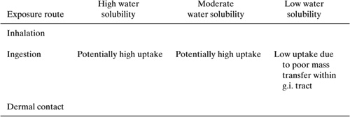
10. The process line shown in Figure Problem 10 delineates the steps in the formulation and packaging of a primer coating for metal parts.
(a) Identify all possible sources of occupational exposure to hazardous chemicals and indicate if exposure is due to inhalation, dermal contact, or other route.
(b) Identify all possible sources of releases to the environment and indicate if the release is to the air, water, or land.
11. The process line shown in Figure Problem 11 delineates the steps in the coloring of leather with dyes.
(a) Identify all possible sources of occupational exposure to hazardous chemicals and indicate if exposure is due to inhalation, dermal contact, or other route.
(b) Identify all sources of releases of hazardous chemicals to the environment and indicate if the release is to the air, water, or land.
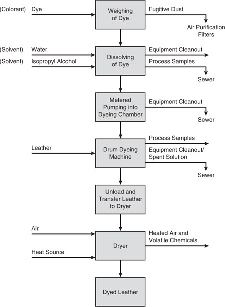
Figure Problem 10 Formulation and packaging of a primer coating for metal parts.
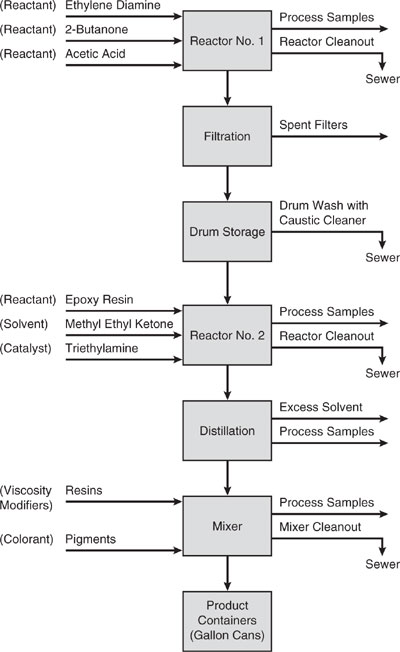
Figure Problem 11 Coloring of leathers and dyes.