
Previous Chapter
Chapter 4: Prediction of photovoltaic power generation output and network operation
Chapter 5
Prediction of wind power generation output and network operation
Ryoichi Hara Graduate School of Information Science and Technology, Hokkaido University, Hokkaido, Japan
Abstract
First, this chapter summarizes the difficulties in power system operation associated with the wind power penetration and the necessity of wind power forecasting that is derived as a solution for these difficulties. Then, the overview of wind power/wind farm output fluctuation characteristics is discussed with various indices showing some related analysis and discussions. Research and development trend in fluctuation suppression techniques is also introduced based on the paper survey results. Finally, the types of wind power forecasting approach is described with example results obtained from the demonstration project conducted in Japan.
Keywords
wind power generation
wind power forecast
fluctuation suppression technology
scheduled generation
5.1. Need for forecasting wind power output in electric power systems
Wind power generation, which can convert the kinetic energy of wind into electric energy without serious environmental damages, is regarded as one of the most promising distributed energy resources in the world. Relatively cheap installation cost accelerates the installation of wind power generation in the world. The Global Wind Energy Council reported that the annual global installed capacity in 2014 exceeded 50 GW and the global cumulative wind power generation capacity has grown exponentially as shown in Fig. 5.1 [1].

Figure 5.1 Global growth of wind power generation.
(a) Annual installed capacity; (b) cumulative installed capacity.
(a) Annual installed capacity; (b) cumulative installed capacity.
Wind power generation appeals because of its merits in cost, ecological compatibility, sustainability, enormousness, and ubiquity natures; however, disadvantages such as intermittency, variability, and uncertainty still remain technological issues. As introduced in Section 5.2.1, power generated from wind power varies depending on the wind speed variation.
In a typical electric power systems, the total generation output of conventional generators such as thermal, hydro, and/or nuclear power plants must meets the total demand (electricity consumption) at every moment to maintain the system frequency. The system operator achieves adequate frequency regulation by the weekly/daily generation scheduling including unit commitments, the online economic load dispatch, and the frequency control based on the speed–droop characteristics, which cover different time domains. The purpose of generation scheduling is to find the most economical generation schedule that can meet the forecasted demand in the coming week/day and satisfy the static and dynamic operational constraints such as capacity limits, voltage limits, procurement of regulation margin, and other criteria on stability, reliability, and security. Here, the demand forecast considered in the scheduling process should be the forecasts for demand that is to be supplied by the conventional generators, or the net demand (the actual demand minus the total output of renewable energy generation systems). That is, the wind power output during the targeted period must be forecast with the same or higher temporal resolution (typically 30 min in daily scheduling process) in the power system with mass penetration of wind power generations. Since the forecast data used in the generation scheduling contains errors, the system frequency deviates even though the generators are running as scheduled. The online economic load dispatch revises the generation schedule based on the short-term (from several minutes to several hours ahead, depending on the country and region) demand and wind power forecasts. Fluctuation of net demand during the scheduling interval also affects the system frequency. As wind power generation grows, the short-term net demand variation is also widened. This short-term frequency deviation is covered by means of the primary and secondary load frequency controls, in which the generator output is automatically regulated within the primary and secondary reserve margin procured in the generation scheduling process. That is, understanding the characteristics of wind power output fluctuation is also an important factor to estimate the adequate level of reserve margins.
As described above, the wind power output forecast is becoming an important technology for the stable operation of power system with mass wind power generations. Actually, some regional system operator (RSOs)/independent system operator (ISOs) and transmission system operator (TSOs) such as Bonneville Power Administration, Electric Reliability Council of Texas, and New York ISO in the United States, Alberta Electric System Operator in Canada, 50Hertz in Germany, EirGrid in Ireland, Energinet in Denmark, Tohoku-EPCO in Japan, and so on, have integrated the wind power output forecasting function into their generation scheduling and/or online economic load dispatch operations [2].
Another need for wind power output forecast is emerging from the wind farm owner/investor side. In some countries and regions, the wind farm is allowed to sell their power at the day-ahead electricity market, to where the market participants have to show their generation schedule in the next day. For wind farms, a generation schedule should be planned based on the day-ahead wind power forecast. If the intraday market becomes more popular, needs for short-term forecast would also emerge.
5.2. Power output fluctuation characteristics
5.2.1. Fundamentals
Theoretically, the available power, Pa (W), in the wind can be expressed as follows:
 (5.1)
(5.1)where, A is the area wind passing through (which is considered perpendicular to the direction of the wind) (m2), ρ is the density of air (kg/m3), and V is the wind speed (m/s). The Eq. (5.2) represents that P is equal to the kinetic energy possessed by the volume of air passing through A per every second. The actual power generation by single turbine generator is, needless to say, less than the above available power. Reasons for this reduction is not only energy conversion losses that consists of mechanical loss associated with bearing and gearbox and cupper and iron losses of generator, but also the electromechanical characteristics of wind power generator; cut-in and cut-out wind speeds and rated power. The cut-in wind speed is the minimum wind speed at which the turbine blades overcome friction and begin to rotate. The cut-out speed is the wind speed at which the pitch angle of turbine blades are regulated to flat to avoid damage from high pressure of wind and the generation is stopped. The actual wind power generation, P (kW), in the steady state is then expressed as follows:
 (5.2)
(5.2)where, Vcut-in and Vcut-out are the cut-in and cut-out wind speeds (m/s), Vrated is the wind speed (m/s) at which the wind power output reaches to the rated power Prated (W), and η is the total conversion efficiency of wind power generator and its associated mechanical transmissions (note that conversion efficiency is also a function of wind speed indeed). For the wind speed Vrated < V < Vcut-out, the pitch angle control maintains the wind power output at Prated. For example, the relationship between P and V, called the power curve, is illustrated in Fig. 5.2. IEC 61400-12 standardizes the wind power output measurement in detail [3]. As observed in Fig. 5.2, the wind power output strongly depends on the wind speed, and therefore, it would vary moment to moment. Fig. 5.3 shows the actual power output of single 1500 kW wind power generator for 10 days [4].
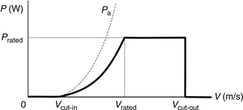
Figure 5.2 Example of power curve of single wind power generator.

For a wind farm, where multiple wind power generators are aggregated together and interconnected to the main grid through the common connection point, the fluctuation of total generation output would be smoothed as shown in Fig. 5.4, which shows the total output of six wind power generators including the generator shown in Fig. 5.3. In detail, the outputs in both figures are similar in trend, but the jaggy (short-term) fluctuation observed in the single generator output disappears in the aggregated output. This is because the short-term fluctuations among generators are uncorrelated due to the spatial dispersion while the long-term trends of output are correlated and similar. Note that the absolute width of fluctuation of synthetic output is statistically wider than those of individual outputs, but the ratio of the fluctuation width to the total capacity (or the mean output), called the relative fluctuation width, becomes narrower than those of individuals. Due to this smoothing effect brought by the geographical dispersion, the shape of the power curve of a wind farm becomes relatively gentle as shown in Fig. 5.5. It can be generally said that a greater number of wind power generators and farther placement would reduce the short-term fluctuation width measured in ratio to the capacity.


Figure 5.5 Example of power curve of a wind farm.
5.2.2. Maximum variation
One of the indices used in fluctuation measurement is the maximum variation, which is defined as a maximum stepwise change of generation output within the specified duration. The maximum variation, which is measured in kW, can represent the impact to the power system directly and intuitively. For stable and safe operation of the power system, the system operator must procure the adequate capacity of reserve, which can cover the maximum variation (more precisely, larger than the maximum variation of net demand) even though the event is an extreme case. The literature [5] summarizes the maximum variations in some countries as shown in Table 5.1. Even in power systems with a large number of sites, the maximum variation of total wind power output is small (about 10%) in shorter timescale (in the order of minutes). In a longer timescale perspective, however, it would reach to 70% in the worst case within 4 h.
Table 5.1
Extreme Variations of Large-Scale Regional Wind Power as a Percent of Installed Capacity
| 10–15 min | 1 h | 4 h | 12 h | |||||||
| Region | Region size (km2) | Number of sites | Max decrease (%) | Max increase (%) | Max decrease (%) | Max increase (%) | Max decrease (%) | Max increase (%) | Max decrease (%) | Max increase (%) |
| Denmark | 300 × 300 | >100 | −23 | +20 | −62 | +53 | −74 | +79 | ||
| West Denmark | 200 × 200 | >100 | −26 | +20 | −70 | +57 | −74 | +84 | ||
| East Denmark | 200 × 200 | >100 | −25 | +36 | −65 | +72 | −74 | +72 | ||
| Ireland | 280 × 480 | 11 | −12 | +12 | −30 | +30 | −50 | +50 | −70 | +70 |
| Portugal | 300 × 800 | 29 | −12 | +12 | −16 | +13 | −34 | +23 | −52 | +43 |
| Germany | 400 × 400 | >100 | −6 | +6 | −17 | +12 | −40 | +27 | ||
| Finland | 400 × 900 | 30 | −16 | +16 | −41 | +40 | −66 | +59 | ||
| Sweden | 400 × 900 | 56 | −17 | +19 | −40 | +40 | ||||
| US Midwest | 200 × 200 | 3 | −34 | +30 | −39 | +35 | −58 | +60 | −78 | +81 |
| US Texas | 490 × 490 | 3 | −39 | +39 | −38 | +36 | −59 | +55 | −74 | +76 |
| US Midwest+OK | 1200 × 1200 | 4 | −26 | +27 | −31 | +28 | −48 | +52 | −73 | +75 |

Denmark, data 2000–2002 from http://www.energinet.dk; Ireland, Eirgrid data, 2004–2005; Germany, ISET, 2005; Finland, years 2005–2007; Sweden, simulated data for 56 wind sites 1992–2001; United States, NREL years 2003–2005; Portugal, INETI.
5.2.3. Umbrella curve
While the maximum variation is used to measure the possible fluctuation deterministically, the distribution of fluctuation magnitude with its occurrence probability is also often used to understand the characteristics of output fluctuation. The umbrella curve, presenting the occurrence frequency of changes in average wind power output during a certain period, is widely used. An example of an umbrella curve is shown in Fig. 5.6, which is reported in Ref. [6]. As illustrated in Fig. 5.6, the distribution of output fluctuation is generally different from the normal distribution and spreads wider.

5.2.4. Standard deviation
One of the important statistical indices for output fluctuation is the standard deviation (SD), defined as follows:
 (5.2.3)
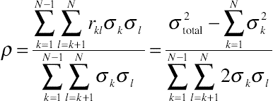
where, Pm is the wind power output (W) measured at mth sampling, Pave is the average output (W), and M is the number of samples. For SD of total output from N generators (σtotal), the following equation can be derived from Eq. (5.2.3):
 (5.2.4)
where, σk is SD of output at kth generator (W), rkl is the correlation coefficient between kth and lth generators. Here, assume that the SD of each generator is identical, that is, σk = σl = σ. When the output from N generators are completely correlated (rkl = 1),
On the other hand, in case of total uncorrelated situation (rkl = 0), total output can be well smoothed, then
In most cases, the outputs of multiple generators are partially correlated as discussed in Section 5.2.5; as a result, ratio of total SD to individual SD stays between  and N. For the aggregation of generators in different size and fluctuation characteristics, the following average correlation coefficient ρ is sometimes used in analysis.
 (5.2.7)
5.2.5. Power spectral density
In some analysis, the fluctuation of wind power generator/wind farm output is studied as the power spectral density (PSD, or simply called the power spectrum in some literature). The terminology “power spectrum” is not the spectrum of power produced, but the square of spectrum magnitude ( ) obtained by the discrete Fourier transform shown in the following equation:
 (5.2.8)
where, f is the frequency (Hz), fs is the sampling rate (Hz), and j is the imaginary unit (j2 = −1).
Literature [4] revealed that the PSD of wind farm output, shown in Fig. 5.7, shows good agreements with Kolmogorov spectrum that can express the characteristics of turbulence of incompressible fluidities and is proportional to  .
.

Figure 5.7 Power spectral density of wind farm with six turbines (gray points) and f − 5/3 spectrum (solid line) [4].
Parseval’s theorem assures that the variance of Pi and the sum of PSD are identical; that is, the PSD can be recognized as the decomposition of variance in the frequency domain. This idea naturally evolves Eq. (5.2.4) into the analogical expression for power spectra of N aggregated output and individuals, as follows.
 (5.2.9)
Where, Stotal and Sk are the power spectra of total and individual outputs, and  and
and  are the coherent and phase angle between two individual outputs. The literature [7] develops a similar extension to Eq. (5.2.7) and reaches to the idea of average coherent (cohav), defined as
 (5.2.10)
Due to the above definition, the average coherence represents the degree of correlation at the specified frequency and ranges from 0 (uncorrelated) to 1 (correlated). The literature [7] also analyzes the average coherent for the 16 wind farms in Hokkaido, Japan, placed over some hundreds of kilometers apart. The major conclusion is that the average coherence for periods longer than 100 min is different day by day, but is relatively high compared with shorter periods. Especially the average coherent for periods less than 10 min is quite small; that is, the smoothing effect by geographical dispersion can only be expected for periods less than 10 min. Distributions of average coherent in different three days reported in Ref. [7] are shown in Fig. 5.8.

5.3. Power output smoothing control
5.3.1. Application of energy-storage system
One of the major fluctuation smoothing approaches is to use the energy-storage system, such as lead–acid, nickel cadmium, lithium ion, sodium sulfur batteries, and ultra capacitor [8–14]. Most energy-storage systems work with DC, therefore, the bidirectional DC/AC converter is needed in principle. Fig. 5.9 shows a typical circuit topology of wind power generator with energy-storage system. Another choice of circuit topology available for a double-fed induction generator or a permanent magnet synchronous generator, which has a DC-link inside, is to embed the energy-storage system into the DC-link as shown in Fig. 5.10. The advantage of the latter topology is to save the system cost and volume, by sharing the DC/AC converter with the generator. For a wind farm consisting of multiple wind power generators, it is beneficial to install single energy system to the farm with the circuit topology as in Fig. 5.9.

Figure 5.9 Circuit topology of wind power generator with energy-storage system connected to AC line.

Figure 5.10 Circuit topology of wind power generator with energy-storage system embedded at DC-link.
A control strategy for an energy-storage system is to charge or discharge the difference between the actual output (P) and the reference output (Pref), as illustrated in Fig. 5.11. The capacity limiter maintains the charge/discharge power with in the inverter capacity. The SOC (state of charge) limiter is also used to avoid overcharging and overdischarging. Several approaches have been developed for deciding reference output; the most major and popular approach is to employ the moving average of actual output. The advantage of moving the average method is the simplicity of the SOC management since the average charged and discharged energy can be balanced automatically in principle. Strictly speaking, the SOC is drifting to empty due to charging/discharging efficiency even if the moving average is applied. For this reason, it is beneficial to implement the SOC feedback control [11] in parallel with Fig. 5.11.

Figure 5.11 Control of energy-storage system for fluctuation smoothing.
5.3.2. Kinetic energy of wind turbines
Needless to say, the wind generator is driven by the wind turbine, whose moment of inertia is relatively large. Thus, the inertia of the wind turbine itself can store energy in the form of kinetic energy. The idea is to store excess wind power by increasing the rotation speed of turbine, and compensate the deficient wind power by decreasing the rotation speed [18,19]. The rotation speed of turbines can be controlled by regulating the generator output while the turbine is receiving the optimal mechanical torque from the wind.
5.3.3. Pitch angle control
Pitch angle control is usually used to maintain the output at rated power for the wind speed higher than the rated speed (Vrated), as shown in Fig. 5.2. Implementation of pitch angle control to the wind speed below the rated speed can realize the constant (or smoothed) output control for wider wind speed range, as shown in Fig. 5.12. The merit of the pitch angle is simplicity of implementation since it does not require any additional devices such as energy-storage system. However, the pitch angle control for smoothing is associated with abandoning the available energy of wind; as a result, this method sacrifices the energy production. In order to avoid unnecessary energy loss, sophisticated pitch angle control schemes have been developed [20–22].

Figure 5.12 Image of power curve with pitch angle control for output smoothing.
5.4. Forecasting methods
5.4.1. Difficulties
Wind power output forecasting is fundamentally the forecasting of wind speed and direction at the location of wind power generator or wind farm during the short time intervals.
For short-term forecasting, which is employed in the online economic load dispatch, atmospheric behavior in a relatively small area must be forecast. Such small area forecasting requires precise and high geographical resolution meteorological measurement data, such as input variables, which are difficult to obtain.
For the day-ahead forecasting, which is used in the generation scheduling, atmospheric behavior in regional size, from mesoscale to synoptic scale, must be forecast. In most region/countries, these are measured, forecast, and provided by a governmental agency; however, their geographical resolution is sometimes coarse to use for the wind generator/farm output forecasting. Furthermore, the length of the temporal horizon (look-ahead period) itself makes forecasting more difficult.
Against the above difficulties, there has been much research and many developments. Of these efforts, there have been two major approaches: physical and statistical. Most wind power forecasting methods fall into one of them, or a combination of both.
Another side to difficulties arises when the system operator tries to forecast the total wind power output in its control area. A straightforward approach is to obtain and sum the output forecasts of all wind farms. In this approach, however, the system operator would handle the mess of the data and require long computation cost. Furthermore, the system operator could not acquire the specifications or online status of some wind farms.
5.4.2. Physical approach
In the physical approach, atmospheric behavior is firstly forecast by numerically solving a set of differential equations representing the state and movement of atmosphere in a the region under consideration, which is modeled by the three-dimensional grid cells with a finite space resolution. In detail, the considered differential equations consist of equations of atmosphere motion (for three dimension), conservation of mass, state equation and thermodynamics of atmosphere, and conservation of water vapor (seven equations) with wind speed (in three dimensions), temperature, pressure, density, and water vapor (seven state variables) for each grid cell. This prediction is called the Numerical Weather Prediction (NWP) and is generally provided by a governmental organization/agency service.
Then, the obtained wind speed at the nearest grid point is scaled considering the hub’s height and the property of terrain, such as the roughness, orography, and obstacles. The refined wind speed is then applied to the power curve of the target wind generator to obtain the wind power output forecast. In order to eliminate the effect of systematic error associated with the NWP modeling and improve the forecast accuracy, a postprocessing named Model Output Statistics (MOS) would be applied. For MOS, one of the statistic approaches described in the next section is applied. The whole organization of the physical approach is illustrated in Fig. 5.13 [23].

Figure 5.13 Structure of physical approach.
5.4.3. Statistic approach
Applying fine temporal and special mesh resolutions in the NWP may improve the forecast accuracy; however, the computation burden would become heavier. In order to shorten the computation time, some statistical approaches have been developed. A statistical approach predicts the wind speed or wind power output simply based on the input data. Statistical approaches are used (1) as a MOS in the physical approach, or (2) as a stand-alone predictor that uses the recent wind condition data (speed and direction). For a MOS application, artificial neural networks (ANNs), multivariable regression models, support vector machines, and fuzzy reasoning techniques are major technologies. For a stand-alone predictor, the autoregressive model or ANN is often employed.
Another form of statistical approach is the forecast ensemble method, in which multiple forecast wind speeds or outputs are composed to obtain the final forecast, as shown in Fig. 5.14. The idea of the ensemble method assumes that the error included in individual forecast is unbiased and uncorrelated, and therefore, composite forecast includes fewer errors. Two strategies can be considered to obtain the multiple forecasts: one is to employ the different forecast methods and another is to vary the input data within their range of uncertainty [24].

Figure 5.14 Structure of ensemble forecast.
5.4.4. Regional forecasting
For the system operator, the target of forecasting would be the total wind power outputs in the control area. However, it is not an easy task for the system operator to sum the output forecasts of all wind farms for several reasons (see Section 5.4.1). Thus, for regional forecasting, the output of reference wind farms is forecast and then the upscaling technique is applied. The literature [23] summarizes the upscaling frameworks in detail.
5.4.5. Probabilistic forecast
In the preceding examples of forecasting, only a single point value is provided for each time interval, which can be regarded as the mean of the conditional distribution of the wind power. However, recent research has focused on forecasting the probabilistic distribution of wind power during the targeted time interval. This type of forecasting is called probabilistic forecast. Major variations of probabilistic forecast provide one or some of the following properties as a forecast: (1) mean, variance, skewness, and or kurtosis, (2) value at risk (quantiles), (3) confident interval, and (4) probability density function or cumulative distribution function. More detailed explanations are found in [23].
5.5. Examples of forecasted results
The Ministry of the Environment of Japan promoted a demonstration project named “wide-area operation systems for multiple renewable energy power plants” in financial year 2012–2014. The primary purpose of this project is the development of a new control system for smoothing the total generation output of multiple wind and solar power plants with the help of weather forecasts and energy storage [25]. The targeted three wind farms are (1) 1980 kW, (2) 2200 kW, and (3) 1200 kW in size and are located in the Hokkaido area of Japan. Two 1000 kW solar power plants are also considered. All five renewable energy power plants are sited at different locations in Hokkaido, and the longest distance is hundreds of kilometers. In this project, day-ahead wind output forecasting system has been developed and run for 1 year to evaluate the forecast accuracy. The developed day-ahead forecasting system can provide average wind power outputs during 30 min intervals in the next day (48 intervals) at 4:00 pm. That is, look-up period ranges from 8–32 h. The developed forecasting system has adopted the physical approach that employs SYNFOS-3D (developed by Japan Weather Association, the spatial resolution is 5 km and the temporal resolution is 1 h) with correction based on the observation data [26].
Fig. 5.15 shows the obtained forecasts and the actual outputs at each wind farm for 1 month. Trends of forecast and actual output are similar, but some large error can be still observed (Jan 17th at site C, for example). A histogram of the normalized forecast errors at each site, shown in Fig. 5.16, presents the quite large (greater than 90%) errors that could be included in the forecast. When all three wind farms results are combined together, as shown in Fig. 5.17, the agreements between the forecast and actual output are improved. This is because the forecast errors at individual sites are not correlated with each other. In statistics, the normalized root mean square errors (RMSE) of each site are 19.5, 19.1, and 18.3%, but in the sum of three sites, the RMSE is reduced to 13.1%.
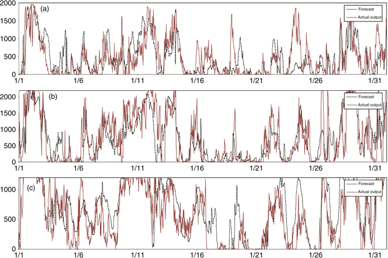
Figure 5.15 Forecast (dash) and actual (solid) wind farm outputs (kW in vertical) in January.
(a) Site A; (b) site B; (c) site C.
(a) Site A; (b) site B; (c) site C.

Figure 5.16 Normalized frequency (vertical) of the normalized forecast errors (percentage in horizontal) counted through 1 year.
(a) Site A; (b) site B; (c) site C.
(a) Site A; (b) site B; (c) site C.

Figure 5.17 (a) Forecast and actual total output in January and (b) the normalized frequency of forecast errors for total output (counted through 1 year).
5.6. Forecasting applications
5.6.1. Scheduled generation of wind farms and solar power plants with energy-storage systems
The literature [25] investigates the scheduled generation operation, in which the total generation output is compensated by the energy-storage systems is regulated to meet the generation schedule, specified 1 day ahead. In this scheduled generation, the generation schedule is made with a 30-min interval based on the day-ahead output forecasts. Both the 30-min energy imbalance and the standard deviation of instantaneous total output during the 30-min interval are used as performance indices. Computer simulations based on the observed field data and output forecasts reveal that, it is not the short-term fluctuation but the error in forecast that has a significant impact on the performance of scheduled generation. As described in Section 5.5, aggregation of wind farms has the potential to mitigate the relative forecast error; therefore, the wide-area forecast and operation are possible solutions in the future. Another option to reduce the effect of forecast error is to introduce the probabilistic forecast. Confident interval or quantile information may provide useful information for more safety side (pessimistic) generation scheduling.
5.6.2. Suppression of ramp variation of wind output
The New Energy and Industrial Technology Development Organization of Japan has launched the demonstration project named “R&D Project on Grid Integration of Variable Renewable Energy: Mitigation Technologies on Output Fluctuations of Renewable Energy Generations in Power Grid” since financial year 2014 (5-year project). One of the primary purposes of this project is to mitigate the wind power output fluctuations, especially the ramp variation (relatively slow output variation, from tens of minutes to several hours) with the help of energy-storage systems. For this kind of application, it is expected that the wind power forecast could contribute considerably. When the ramp variation cannot be forecast, the energy-storage system must begin its compensation behavior right after the detection of ramp variation, as shown in Fig. 5.18a. In this case, the energy-storage system must store or release the energy corresponding to the hatch area. If the occurrence of ramp variation can be anticipated in advance and the compensation by energy-storage system can be initiated earlier, as shown in Fig. 5.18b, the necessary compensation power and energy could be reduced significantly (in Fig. 5.18b, only 50% of the kilowatt capacity and 25% of the energy capacity are required compared with Fig. 5.18a).

Figure 5.18 Image of compensation of step-wise variation of wind power output by energy-storage system.
(a) After the variation detection and (b) before the variation with the support of output forecast.
(a) After the variation detection and (b) before the variation with the support of output forecast.
..................Content has been hidden....................
You can't read the all page of ebook, please click here login for view all page.