
Chapter 6
Energy management systems for DERs
Atsushi Yona Department of Electrical and Electronics Engineering, Faculty of Engineering, University of the Ryukyus, Okinawa, Japan
Abstract
When connecting power plants of distributed energy source to existing power systems, we should consider the energy management. This chapter describes application methods about energy management concentrating on home energy management systems (HEMS), energy storage systems, electric vehicles, and smart meter data. This chapter starts by explaining the basic concepts of HEMS. In Section 6.2, control strategies for energy storage systems are described. Section 6.3 introduces application example of electric vehicles. Finally, Section 6.4 summarizes the use of smart meter data.
Keywords
home energy management systems (HEMS)
storage
smart meters
distributed generators (DGs)
power
When connecting power plants of distributed energy source to existing power systems, we should consider the energy management. This chapter describes application methods about energy management concentrating on home energy management systems (HEMS), energy storage systems, electric vehicles (EVs), and smart meter data. This chapter starts by explaining the basic concepts of HEMS. In Section 6.2, control strategies for energy storage systems are described. Section 6.3 introduces application example of EVs. Finally, Section 6.4 summarizes the use of smart meter data.
6.1. Basic concepts of home energy management systems
Due to a fluctuating power from distributed energy sources such as renewable energy sources and loads, supply/demand balancing of power system becomes unstable. Kenichi Tanaka et al. [1] proposed a methodology for optimal operation of a smart grid to minimize the interconnection point power flow fluctuation. The system consists of basic concepts of HEMS including photovoltaic (PV) generator, heat pump (HP), battery, solar collector (SC), and load. For further research and dissections, Refs. [2–9] review work for basic concepts of HEMS. Marc Beaudin et al. [2] have written a review of modeling and complexity of HEMS. A. Tascikaraoglu et al. [3] introduced the concept for a demand side management strategy of smart home system in Turkey. Yumiko Iwafunea et al. [4] discussed, in considerable detail, cooperative home energy management using batteries for a PV system. Rim Missaoui et al. [5] explained in detail the performance analysis of a global model-based anticipative building energy management. Hanife Apaydın Özkan [6] provided a real-time solution to reduce the electricity cost and to avoid the high peak demand problem simultaneously for a smart home. Phani Chavali et al. [7] presented distributed energy scheduling algorithm as a demand response for the smart grid, and Mohammad Chehreghani Bozchalui et al. [8] proposed hierarchical control approach for energy management of greenhouse. The proposed model incorporates weather forecasts, electricity price information, and the end-user preferences to optimally operate existing control systems. Amjad Anvari-Moghaddam et al. [9] applied a multiobjective mixed integer nonlinear programming model to optimal energy in a smart home considering a balance between energy saving and a comfortable lifestyle.
This section summarizes Ref. [1] as an example of HEMS. In the Ref. [1], the authors present an optimal operation method of the direct current (DC) smart house group with the controllable loads in the residential houses as a smart grid. The DC smart house consists of a SC, a PV generator, a HP, and a battery. The HP and the battery are used as controllable loads in this research. The proposed method has been developed in order to achieve the interconnection point power flow within the acceptable range and the reduction of max–min interconnection point power flow error as low as possible to smooth the supply power from distribution system. Power consumption of the controllable load is determined to optimize the max–min interconnection point power flow error based on the information collected from power system through communication system. By applying the proposed method, we can reduce the interconnection point power flow fluctuation, and it is possible to reduce electricity cost due to the reduction of the contract fee for the electricity power company. Also, by using battery as the power storage facility, which can operate rapidly for charge and/or discharge, the rapid output fluctuations of DC load and PV generator are compensated. The smart grid model is shown in Fig. 6.1. The smart grid has six smart houses, and is connected to the power system and control system through a transmission line and communication infrastructures. The control system sends required control signals to the smart house group which response to the system’s conditions. Each smart house determines the operation of controllable loads. The interconnection point power flow is the power flow from the power system to the smart grid in Fig. 6.1. The DC smart house model is shown in Fig. 6.2, which consists of a DC load, a PV generator, an SC, an HP, and a battery. The HP and the battery are used as controllable loads.


Fig. 6.3 shows the numerical model of SC system. It is assumed that sum of total solar radiation will be falling on the SC and array, and it does not consider the incidence angle of SC array. Optimal operation of smart grid is determined to minimize the interconnection point power flow fluctuations. Due to reduce the interconnection point power flow fluctuation, it is possible to suppress the harmful effects to power system, and it is possible to reduce electricity cost.

Furthermore, the proposed configuration of electricity price as shown in Fig. 6.4 assumes the smart grid system in the future. If the interconnection point power flow within the bandwidth (Region A) has an electricity purchase cost of 10 Yen/kWh, and if the interconnection point power flow departs from the bandwidth (Regions B and C), the electricity purchase costs are 20 and 30 Yen/kWh, respectively. Moreover, the electricity selling cost to the power system is 10 Yen/kWh. The bandwidth is given by power system to smart grid as power reference. Therefore, it is important that the customer follows the power reference and interconnection point power flow within the bandwidth.

Tabu Search (TS) with local search methodology, which always moves neighborhood solution, is used as the optimal technique to address the problems of determining the charge/discharge power of battery and HP operation time for each smart house. It is possible to determine heating time of an HP by assuming power consumption, except controllable loads and heat load which could be forecast. Therefore, the charge/discharge power of the battery and HP operation time for each smart house are calculated by using TS under the objective function and constraints. Simulation results for sunny, cloudy, and rainy weather conditions are shown in Figs. 6.5, 6.6, and 6.7, respectively. Assuming power consumption except controllable loads and PV output power in each weather conditions are shown in Figs. 6.5(a), 6.5(b), 6.6(a), 6.6(b), 6.7(a) and 6.7(b), respectively. These figures show power consumption except controllable loads and PV output power in smart grid and each smart house, respectively.

Figure 6.5 Simulation results in sunny weather condition [1].
(a) Power consumption except controllable loads; (b) PV output power; (c) water temperature of HP; (d) power consumption of HP; (e) supplying power from infinite bus; (f) remaining energy capacity of battery.
(a) Power consumption except controllable loads; (b) PV output power; (c) water temperature of HP; (d) power consumption of HP; (e) supplying power from infinite bus; (f) remaining energy capacity of battery.
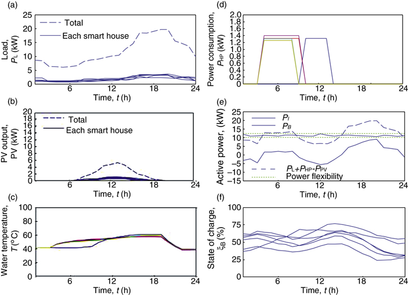
Figure 6.6 Simulation results in cloudy weather condition [1].
(a) Power consumption except controllable loads; (b) PV output power; (c) water temperature of HP; (d) power consumption of HP; (e) supplying power from infinite bus; (f) remaining energy capacity of battery.
(a) Power consumption except controllable loads; (b) PV output power; (c) water temperature of HP; (d) power consumption of HP; (e) supplying power from infinite bus; (f) remaining energy capacity of battery.

Figure 6.7 Simulation results in rainy weather condition [1].
(a) Power consumption except controllable loads; (b) PV output power; (c) water temperature of HP; (d) power consumption of HP; (e) supplying power from infinite bus; (f) remaining energy capacity of battery.
(a) Power consumption except controllable loads; (b) PV output power; (c) water temperature of HP; (d) power consumption of HP; (e) supplying power from infinite bus; (f) remaining energy capacity of battery.
It is possible to reduce the cost with the proposed control because the interconnection point power flow is controlled within the bandwidth by operating controllable loads. In sunny weather conditions, PV power output and SC heat generation are high due to sufficient solar radiation. Therefore, it is not necessary to heat by HP and the power consumption for each house is not increased any more. So, the sunny weather condition is the lowest cost in the three cases. Power consumption in smart grid is smoothed by achieving the proposed method, so we can suppress the impact of PV against the power system. Consequently, we can expect high quality power supply and reduce the cost by cooperative control in the smart grid.
6.2. Control strategies for energy storage systems
When renewable distributed generators (DGs) are connected to the power system, there is a concern about their harmful effects as most of their power fluctuates with weather conditions. Therefore, many researchers have been working on practical application of microgrids. Kyohei Kurohane et al. [10] proposed a DC microgrid with renewable energy. The proposed method is composed of a gearless wind power generation system and a battery in a DC distribution system. The battery helps to avoid DC overvoltages by absorbing the power of the permanent magnet synchronous generator (PMSG) during line fault. The proposed system presents a control strategy based on the maximum power point tracking (MPPT) control to generate the maximum power for the variable wind speed and a pitch angle control to smooth the output fluctuation at low wind speed. The system consists of control strategies for energy storage systems. For further research and dissections, Refs. [11–15] discuss control strategies for energy storage systems. Yu Zheng et al. [11] proposed battery energy storage system (BESS)-based energy acquisition model for the operation of distribution companies in regulating price considering energy provision options, and the results show that the capacity requirement is reduced. Sathish Kumar Kollimalla et al. [12] introduced the concept of a hybrid energy storage system. In the method, batteries are used to balance the slow changing power surges, whereas supercapacitors are used to balance the fast changing power surges. Ayman B. Eltantawy et al. [13] discussed in method for increasing the capacity of small-scale renewable distributed generation sources that can be installed in distribution systems based on both a technical and economic assessment. Xinda Ke et al. [14] discussed in detail the control algorithms and sizing strategies for using energy storage to manage energy imbalance for variable generation resources. Zhaoyu Wang et al. [15] presented a decentralized power dispatch model for the coordinated operation of multiple microgrids and a distribution system.
This section summarizes Ref. [10] as an example of energy storage systems. The DC distribution system has the following advantages over the alternating current (AC) distribution system. (1) Each power generator connected to the DC distribution system can easily be operated in coordination because it controls only the DC bus voltage. (2) When the AC grid system is faulty, the DC distribution system is disconnected from the AC grid. It is then switched to the stand-alone operation in which the generated power is supplied to the loads connected to the DC distribution system. (3) The system cost and loss can be reduced because only a single AC grid-side inverter unit is needed. With the rapid growth of the wind turbine generator (WTG) systems, it is difficult to stabilize the operation of the power system by disconnecting WTGs when there are line faults. Under the line fault, the dispersed power sources are disconnected from the power system, requiring much more time and energy to compensate for the power supply–demand balance. In addition, with the recovery of the power system, disconnected WTGs need to be restarted. Thus, the frequency of the power system rise as many WTGs return to the system. As a countermeasure, in Europe, large WTGs are required to remain connected to the power system under line fault, and supply power to the power system after fault clearing. This requirement is called fault ride-through. Moreover, under the line fault, the DC bus voltage in the DC distribution system experiences overvoltage. Therefore, unstable power supply from DC distribution system and an overvoltage problem of semiconductor devices of the power converter occur. It is important to solve these problems of the stable operation for DC distribution system. Stable power supply strategies for DC distribution system and stable control strategies for PMSG under the line fault are proposed. The proposed method uses a battery for the DC distribution system. Under the line fault, a chopper circuit is used to avoid DC bus overvoltage by absorbing energy from the PMSG and by supplying to the battery. By means of the proposed method, stable operation of the DC power system under the line fault becomes possible, and a highly reliable power supply can be achieved from the grid-side inverter to the AC grid after the line fault is cleared.
The DC power system used in this study is shown in Fig. 6.8. The wind power generator is a gearless 2 MW PMSG. The PMSG has a simple structure and high efficiency. In addition, the DC distribution system consists of a gearless 2 MW PMSG, a grid-side inverter, a 576 Ah battery and 100 kW DC loads. The DC system is connected to a 10 MVA diesel generator and 5 MW AC loads through the grid-side inverter. Wind power energy obtained from the windmill is sent to the PMSG. In order to generate maximum power, the rotational speed of the PMSG is controlled by the pulse width modulation (PWM) converter and the generated power is leveled by a pitch angle control. This power is then supplied to the DC load. The rest of the power is supplied to the AC load through the grid-side inverter.

The power converter control systems are shown in Figs. 6.9 and 6.10. Generator-side converter achieves variable speed operation by controlling rotational speed of the PMSG. On the other hand, the grid-side inverter supplies electrical power and its frequency is synchronized with the frequency of the power system. Each of the power converters is a standard three-phase two-level unit, is composed of six insulated gate bipolar transistors (IGBTs), and is controlled by the triangle wave PWM law. In addition, the DC distribution system includes a battery, in order to avoid DC bus overvoltages under line fault.


The battery model is considered for battery’s discharge and charge characteristics. In this study, the authors consider a lithium ion battery. The state of charge (SOC) is calculated by the integration of the discharge and charge power of the battery. The proposed constant DC bus voltage control is achieved by using a bidirectional DC chopper in connection with a battery. The control systems are shown in Figs. 6.11 and 6.12. The bidirectional DC chopper controls the duty ratio for normal operation (SWnormal) or line fault (SWfault). The switching determinations for SWnormal and SWfault are performed by considering the AC grid voltage, vt. When the AC grid voltage is vt ≥ 0.8 pu, the bidirectional DC chopper performs the normal operation. If the AC grid voltage is vt < 0.8 pu, the bidirectional DC chopper performs under the fault operation. Under the line fault, this chopper circuit helps to avoid DC bus overvoltage by absorbing energy from PMSG and supplying it to the battery, keeping the DC bus voltage constant. The rapidly rising DC bus voltage is difficult to keep constant using the only proportional–integral (PI) controller of the AC grid side inverter. The control system under the line fault is shown in Fig. 6.12. In this system, the PWM reference signal 2 is determined by the output of PI11 controller. The output of the comparator 4 depends on the comparison of PWM reference signal 2 and carrier wave signal. The carrier wave signal is 1 when the carrier wave signal is greater than the reference signal, and is 0 when the carrier wave is less than the reference signal. IGBTs are used as switching devices for the DC chopper circuit.


The effectiveness of the proposed method is examined by a switching simulation with the system model shown in Fig. 6.8. This simulation considers that the three-line to ground fault occurs at the middle of transmission line of Fig. 6.8 and electrical power supply to the load is shut down. The sequence of simulation is described further:
1. At t = 5.0 s: The three-line to ground fault occurs at the middle of transmission line.
2. When the AC grid voltage is within vt < 0.8 pu, the gate signals for grid-side inverter are stopped.
3. At t = 5.1 s: The line fault is cleared.
4. When the AC grid voltage is within vt ≥ 0.8 pu, the gate signals for grid-side inverter are restarted.
The simulation results are shown in Figs. 6.13 and 6.14.

Figure 6.13 Simulation results during three-line to ground-fault [10].
(a) Wind speed; (b) active power of PMSG; (c) reactive power of PMSG; (d) DC bus voltage; (e) DC load; (f) terminal voltage of DC load; (g) terminal voltage of battery; and (h) output power of battery.
(a) Wind speed; (b) active power of PMSG; (c) reactive power of PMSG; (d) DC bus voltage; (e) DC load; (f) terminal voltage of DC load; (g) terminal voltage of battery; and (h) output power of battery.
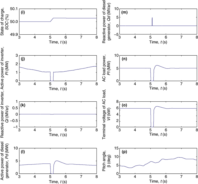
Figure 6.14 (i) State of charge; (j) active power of AC grid-side inverter; (k) reactive power of AC grid-side inverter; (l) active power of diesel generator; (m) reactive power of diesel generator; (n) AC load; (o) terminal voltage of AC load; and (p) pitch angle [10].
In normal operation, the proposed system presents a control strategy based on the MPPT control to generate the maximum power for the variable wind speed and a pitch angle control to smooth the output fluctuation at low wind speed. Besides, at high wind speeds, it is possible to control the output power of the PMSG by the pitch angle control system. In addition to these control strategies, the DC bus voltage is controlled by using a bidirectional chopper and battery under the line fault. From the simulation results, it was confirmed that the DC distribution system with the proposed method can stabilize power system operation under the line-fault and can supply stable power from the grid-side inverter to the power system after the line-fault clearing.
6.3. Control strategies for EVs as storage
In the installation area of a large renewable energy sources, such as a PV system, appropriate operation is required, and it is better to minimize the size of the battery and its capital cost. Atsushi Yona et al. [16] proposed an optimization approach to determine the operational planning of the power output for a large PV system. The approach includes the method of determination of the charge/discharge amount for the battery of an EV as a demand response. The method aims to obtain a more beneficial deal with the sale of electrical power. The operation consists of control strategies for EVs as storage. For further research and dissections, Refs. [17–21] are related with control strategies for EV as storage. Mingrui Zhang et al. [17] proposed a pricing scheme through a fuzzy control method to facilitate the energy management for EVs and battery swapping station based on islanded operation of the microgrid. Preetham Goli et al. [18] proposed a unique control strategy based on DC link voltage sensing with integration of PV and plug-in EVs for efficient transfer energy. Tan Ma et al. [19] have written in detail the economic analysis of a real-time power flow control algorithm for charging a large-scale plug-in EVs network. Kan Zhou et al. [20] introduced decentralized random access framework with charging plug-in EVs to avoid bus congestion and large voltage drop in the distribution grid. Uwakwe Christian Chukwu et al. [21] performed to investigate the real-time management of power systems with vehicle-to-grid (V2G) facilities.
This section summaries Ref. [16] as an example of control strategies for EVs as storage. The authors described an optimal operational planning strategy applying demand response (DR) for a large PV/battery system. The authors assume that the objective function is to maximize the obtained benefit of electrical power selling from the combined power output from the PV system developer and demand from EVs users. At present, the contribution of EVs as a DR is quantified. The required electric power for the initial SOC of the battery is described by simulation, with the result that the purchased power at nighttime is assumed to be available. The forecast power output errors of the PV system for the case of over/under fitting are assumed. The PV power output by MPPT is restrained, considering the variation of combined power output, inverter capacity, and its conversion efficiency, and then the combined power output is smoothed according to the command for charge/discharge of the BESS. A genetic algorithm is applied as the optimization technique to determine the combined power output and initial SOC of BESS. In order to decrease the battery capacity, the proposed technique should be implemented by the aggressive introduction of EVs. The simulation results show the potential of DR as an option to compensate for the PV power output forecast errors for optimal operational planning.
6.4. Use of smart meter data
Due to global warming and the depletion of fossil fuels, we are required to reduce CO2 emissions and energy consumption. To solve these problems, the installation of PV and SC systems in residential houses has been proposed for the demand side. Moreover, the introduction of the HP is also expected as an efficient water-heating appliance. The general electric utility company sets a time-of-use electricity rate system to absorb peak power demand and to operate the thermal power generator at the highest efficiency. Much research has been carried out regarding this matter, pertaining to decreasing peak power demand and to the control of house loads. Consequently, houses with an HP have benefited from the electricity pricing system in residential areas. In addition, if a fixed battery is introduced to houses under this electricity pricing system, the electricity cost for the houses would further decrease because it would be possible to recharge the battery using cheap electricity in the middle of the night. Another recent trend is the increase of occupants who have EVs and who are able to implement the vehicle to home system, which can compensate the power consumption of the houses with the EV battery by attaching it to the grid (V2G). Thus, it is expected that users will be likely to install EVs and fixed batteries with effective utilization strategies in the coming decades. Unfortunately, the investment cost for these appliances is quite high. Thus the installation cost to the consumer is likely to increase. Akihiro Yoza et al. [22] proposed an expansion-planning model of PV and battery systems for the smart house. The expansion-planning period is 20 years and ranges from 2015 to 2035 in Japan. The operation consists of using smart meter data. The proposed method clarifies the optimal installation year, capacity, and appliances during the 20-year period considering variable characteristics such as investment cost, selling price, and purchasing price which change year by year. For further research and dissections, Refs. [23–26] discuss smart meters. Waleed Aslam et al. [23] discussed in detail the smart meter technology and applications across residential, commercial and industrial sectors. Sabine Erlinghagen et al. [24] discussed in considerable detail the identifying wired and wireless communication standards for smart metering in Europe, and described a comprehensive set of criteria for standard selection compared with the existing standards. Myriam Neaimeh et al. [25] have written a probabilistic method to combine two datasets of real EV charging profiles and residential smart meter load demand. Franklin L. Quilumba et al. [26] presented the efforts involved in utilizing the advanced metering infrastructure data to improve the load forecasting accuracy at the system level.
This section shows summary of the Ref. [22] as an example of use of smart meters data. The authors proposed a model of optimal expansion planning of PV and battery systems in a smart house for a 20-year period. The optimization method employs the TS algorithm which is known to be metaheuristic and a model to reduce calculation time is devised. It is assumed that the expansion-planning period ranges from 2015 to 2035. In advance, the smart house contains HP and SC systems. It is assumed that the occupant in the smart houses has a plan to install PV and battery systems. By solving this optimization problem, the optimal installed year, and the most beneficial capacity for the appliances are revealed for 20-year period, and the minimal total payment cost during the expansion period for the consumer is calculated. The yearly varying electricity purchasing price for the consumer and the selling price for the general utility company are considered. In order to verify the effectiveness of the proposed system, MATLAB® is used for simulations.
The smart house system model is shown in Fig. 6.15. The smart house model, which consists of SC, HP, PV, and battery, is used for the expansion problem of the PV and battery on the residential side. The authors assumed the occupant has a plan to introduce PV and a fixed battery system in the house within 20 years, where the HP and the battery are used as controllable loads. From Fig. 6.15, PIt, PLt, PBt, PPVt, and PHPt represent power flow from the power supply to the smart house, power consumption other than controllable loads, charge/discharge power of the battery, PV output power, and power consumption of the HP respectively.

The HP is used for a hot water supply and the standard is a 370 L type with 1.0/4.0 kW heater with a coefficient of performance of 4.0. Moreover, the examined capacity of the PV varies from 0 to 10 kW, and the examined inverter capacity and battery capacity vary from 0 to 3 kW and 0–10 kWh, respectively. It is assumed that the simulation is carried out in Okinawa in Japan where the temperature is comparatively warm and the solar intensity is strong. In addition the season is summer-like in October. Weather data of the Japan Meteorological Agency is used.
The objective function and the constraints for optimization of expansion planning of the appliances are described as follows.
The total cost during an expansion period of 20 years for the occupants is defined as summation of investment and operational cost in the smart house. It is assumed that the expansion-planning period ranges from 2015 to 2035. The optimization problem is to solve for when, what capacity, and which appliances (PV and/or battery) are installed during the two-decade period. Thus, the objective function is set to minimize the total cost and described as follows.
Objective function:
where TC: total cost during 20 years; CINVEST: investment cost for the appliances; COPE: operational cost for the consumer; T: expansion planning period (T = 20, inaugural year is 2015); te: time index (by year); EPV (te): binary variable for PV to be installed in year te; EBA (te): binary variable for battery to be installed in year te; CPV (te): investment cost for PV in year te; CBA (te): investment cost for battery in year te; CPAY (te): electricity payment for the consumer in year te; CPS (te): benefit of sold by PV output power in year te; and CBS (te): benefit of sold by battery discharge power in year te.
The first and second terms mean the investment cost, which is existent according to binary variable representing whether or not the PV or battery system has been installed in year te. The third term means the electricity cost which the occupant pays the utility company in year te. The fourth and fifth term mean the benefit obtained by sold power generated by the PV and battery in year te according to the binary variable, respectively.
The objective function of the constraints for optimal scheduling is depicted as follows.
For the objective function of the optimization of expansion planning, if the installation year is determined, the investment cost can be calculated as CINVEST for the appliances in year te for a short while. However, the operational cost, COPE, which the occupant of the smart house pays during a 20-year period must be simulated at hourly time, t. Thus, the following objective function means minimization of operational cost during a 20-year period in the simulation at hourly time, t.
Objective function:

where T: expansion planning period (T = 20, inaugural year is 2015); te: time index (by year); TY: represents the four seasons in year; TM: days in 1 month including fair, cloudy and rainy day; t: time index (by hour); CP(t,TM,TY,T): cost of purchased power in hour t, month TM, season TY, year T; CS(t,TM,TY,T): benefit of sold power in hour t, month TM, season TY, year T; UP(t,TM,TY,T): unit price for purchased power in hour t, month TM, season TY, year T; and US (t,TM,TY,T): unit price for sold power in hour t, month TM, season TY, year T.
The TS is a metaheuristic global optimization method discovered by Glover, which has been effectively used for a combinational optimization such a scheduling problem. TS can find the optimal solution by carrying out the iteration step until a criterion is achieved. However, this simple iteration may cause the cycling in which the search moves within the same loop among local solutions. In order to prevent this cycling from occurring, a memory system called the tabu list, which records the latest moves, is applied in the searching procedure. The utilization of the tabu list can reduce the probability of going into a local iteration since the highest evaluated solution is selected by referring to the tabu list for the next solution xnex. The following implementation parameters are used for the TS. The global iteration max is 4000 and the length of the tabu list is 500. The optimization problem is encoded into the program based on the algorithm and simulated on MATLAB.
The simulation time becomes very long because an optimal hourly scheduling must be solved for many optimization variables and the operational cost of the smart house during 20 years is calculated with the optimization procedure in hourly steps for a long-term simulation of 20 years. A solution methodology for shortening the simulation time is cubic spline interpolation. The function which calculates the operational cost of smart house for 1 year is used in order to shorten the simulation time. The procedure to derive the function is described in this subsection. First, an optimization for hourly scheduling of controllable loads in the house is solved for many variables with a specific small interval. The variables are the capacity of the PV, battery, electricity purchasing price, and selling price from consumer to utility. The minimum operational costs of the house are obtained from the optimal scheduling of appliances for a year. However, an operational cost which has not been investigated cannot be obtained in combinations of small intervals for these variables. Thus, operational costs for the variables which have not been investigated are estimated with cubic spline interpolation, which is a useful technique to estimate the unknown data from the obtained data. The cubic spline interpolation uses piecewise polynomials such that three order polynomials are each divided into small intervals, continuing for a finite interval.
The optimization flow chart is depicted in Fig. 6.16. At first, the minimal operational cost in various cases is revealed in determining the optimal scheduling of the appliances. After that, the function is then derived as piecewise continuous polynomial by cubic spline interpolation. Next, the solution of the optimization problem of expansion planning for the PV and battery is determined by TS.

Figure 6.16 Flow chart for optimal scheduling and expansion planning [22].
Equation (29) is operational cost (COPE) for the consumer; equation (10) is objective function (TC) for total cost during 20 years.
Equation (29) is operational cost (COPE) for the consumer; equation (10) is objective function (TC) for total cost during 20 years.
Four simulation cases are carried out for the optimization of expansion planning for PV and battery systems. Case 1 has neither PV nor battery installed during the planning period (20 years). Case 2 is the scenario in which the occupant has a plan to install only the PV system during the planning period. Case 3 is the scenario in which the occupant has a plan to install only a battery during the planning period. Case 4 includes both PV and battery installation during the planning period. The detailed simulation conditions are described as follows for the optimization problem of expansion planning.
▪ The selling unit price by feed in tariff (FIT) is kept the same from the year installed until after 10 years, that is, when the contract is finished. After that, the selling unit price of the year is applied and is guaranteed for 10 years.
▪ Once the appliances are installed in the smart house, they are kept as set. Furthermore, the same appliances are not reintroduced (such as two or three times) during the expansion-planning period.
▪ It is assumed that three people use 30 L and 150 L of hot water for showers from 7:00 to 8:00 and from 19:00 to 22:00, respectively, in a smart house. The HP is operated in such a manner that the temperature does not fall below 50°C in the storage tank.
Fig. 6.17 shows that the operational cost of the smart house for each year, which is calculated by solving for optimal scheduling of the appliances at time index hour, t, in advance before the optimization for expansion planning is investigated. It is observed that the operational cost has a trend of increasing from 2015 to 2034 since the purchased electricity unit price becomes expensive. Moreover, if the battery is installed, the operational cost rises since in this case, the sold electricity unit selling price is lower than the unit price of PV due to price system of double generation which means the selling price for a PV only owner is higher than that for the PV and battery owner or battery only owner. This price rate is actually applied in Japan, even if one battery is set in the smart house. Thus, in the case which includes a battery with a capacity of 0 kWh and PV capacity of 10 kW, the operational cost is very beneficial.

Figs. 6.18–6.21 depict the optimal installation year, capacity, investment cost, operational cost during 20 years, and variation during a period of 20 years, respectively. In Fig. 6.20 and Fig. 6.21, a positive cost means that the occupant pays the cost, and a negative cost means that the occupant obtains a benefit. In Case 1, although the investment cost is 0 Yen (see Fig. 6.19), the operational cost becomes expensive during 20 years, and in Fig. 6.20 the total cost is more expensive than any other case (see Fig. 6.21). It can be seen that the case in which the total cost is the least expensive among Cases 2–4 is Case 2 (see Fig. 6.21). The reason for this is that only the PV is installed and the electricity unit selling price is high. In addition, if the PV is installed in 2015, which is beginning year of the expansion planning period, the operational cost would be more reasonable since the selling price decreases year by year. Actually, from Figs. 6.18–6.21, in Case 2 the PV is installed in 2015 and the capacity is 10 kW. On the other hand, in Case 3 the optimized results indicate that the battery should be installed in 2024 and the best capacity is 3 kW/6 kWh. The simulation time to solve the optimal expansion planning of the PV and battery is significantly reduced by 50% to the conventional method.


The optimization problem was separated into two parts, and the optimal scheduling of the appliances is solved in time indices 1 h in advance. In expansion planning optimization, the cost function is derived by scheduling optimization by cubic spline interpolation, and TS is employed as an optimization tool. This research clarified the optimal installation year, capacity, and type of appliances which make a better choice, and solved for the total cost during a period of 20 years in each case for the consumer side.
..................Content has been hidden....................
You can't read the all page of ebook, please click here login for view all page.