Chapter 11

Stability problems of distributed generators

Toshihisa Funabashi*
Jinjun Liu**
Tomonobu Senjyu
*    Institute of Materials and Systems for Sustainability (IMaSS), Nagoya University, Nagoya, Japan
**    Xi’an Jiatong University, Xi’an, China
    Department of Electrical and Electronics Engineering, University of the Ryukyus, Okinawa, Japan

Abstract

Voltage stability covers a wide range of phenomena in power systems. In this chapter, voltage stability problems of distributed generators (DGs) are briefly described. Then, a new voltage-stability-analysis method for DGs connected to a weak power system is explained. An example of analysis is shown. The method uses active and reactive power information of power transmission lines in accordance with the voltage stability. Two proposed stability criteria are explained. Based on the comparison between two proposed stability criteria, a comprehensive understanding about the stability issues of multimodule system is illustrated. For a microgrid composed of inverter-based DGs, transient characteristics are explained. These analyses consider whether microgrid can be self-sustained operation without interruption at fault event.

Keywords

voltage stability
stability criteria
microgrid
inverter-based distributed generators
transient characteristics
self-sustained operation

11.1. Voltage stability in distribution systems

Voltage stability covers a wide range of phenomena and means different things to different engineers [1]. It is a fast phenomenon for engineers involved with induction motors and it is a slow phenomenon for other engineers. Some engineers and researchers have discussed whether voltage stability is a static or dynamic phenomenon. Voltage instability and voltage collapse are used somewhat interchangeably. Voltage stability or voltage collapse has often been viewed as a steady state problem. It was viewed suitable with static power flow type analysis. A CIGRE report [2] recommends analysis methods and power system planning approaches based on static models for voltage collapse prevention. However, the network maximum power transfer limit is not necessarily the voltage stability limit. Voltage instability or voltage collapse is a dynamic problem. Of course, the power system is a dynamic system. In contrast with rotor angle stability (synchronous stability), the dynamics mainly involves the loads and the voltage controllers. The definition of voltage stability is given in CIGRE report [3]. Voltage stability is a subset of power system stability.

11.1.1. Definitions [1]

A power system at a given operating states is small disturbance voltage stable if, following any small disturbance, voltages near loads are identical or close to the predisturbance values. (Small disturbance voltage stability corresponds to a related linearized dynamic model with eigenvalues having negative real parts. For analysis, discontinuous models for tap changers may have to be replaced with equivalent continuous models.)
A power system at a given operating state and subject to a given disturbance is voltage stable if voltages near loads approach postdisturbance equilibrium values. The disturbed state is within the region of attraction of the state postdisturbance equilibrium.
A power system at a given operating state and subject to a given disturbance undergoes voltage collapse if postdisturbance equilibrium voltages are below acceptable limits. Voltage collapse may be total (blackout) or partial.

11.2. Stability problem with DGs connected to a weak power system

Recent liberalization of the power market combined with growing concern about the depletion of energy resources has led to an increase in the introduction of solar power generation in the electric power grid. Moreover, the move to all-electric home systems in the interest of economic benefits results in an increase of demand, causing the power system to operate near power transmission capacity in severe situations [4]. With more efficient use of transmission lines, it is possible that the power systems can be operated near voltage stability limits. As a result the possibility of voltage collapse will increase [1,5]. Therefore, voltage stability analysis is a major consideration in the stable operation of the power system.
Voltage stability has been analyzed in a variety of ways. Some of the analysis techniques include P (Active power)–V (Voltage) analysis, which concerns the relationship of the voltage and active power in the transmission system, and Q (Reactive power)–V analysis, which concerns the relationship of the voltage and reactive power [611]. Indicators of voltage stability proposed in these papers include finding the change in active and reactive power with respect to the change in voltage from the P–V and Q–V characteristics, the proximity of the high and low voltage vectors from the PV characteristics, and the voltage stability margin of the active power that can be consumed by the load. There has been little work done with regards to voltage stability considering both the active and reactive power at the same time because analysis becomes difficult. However, it is expected that accurate voltage stability analysis can be performed considering both the active and reactive powers simultaneously. Because active and reactive power are both main values regarding transmission characteristics, the P–Q characteristics, should also be considered.
We have previously proposed a voltage stability limit index that takes into account the active and reactive power in the transmission [12].
In this section, a method to improve the voltage stability of the power system is presented by using active and reactive power information of power transmission lines in accordance with the voltage stability [13]. Simulation results show that from the actions of charging and discharging with active and reactive power control, the voltage stability of the system can be improved with an appropriately large capacity storage battery installed at substation.

11.2.1. Voltage stability analysis

The model assumed in this section is shown in Fig. 11.1. The Institute of Electrical and Electronics Engineers 5-bus system is used [14]. In a transmission line model, Vi is the sending end voltage and Vj is the receiving end voltage, Pk is the active power being sent to the receiving side, and Qk is the reactive power being sent. The power flow equation of the 2-bus system is expressed by the simple equation. There is a limit to possible transmission power for any given time; that power is called the power stability limit and the voltage is called the voltage stability limit [15]. The P–Q characteristics of the power stability limit are shown in Fig. 11.2. From the P–Q characteristics the relationship between Vi and Pj at the voltage stability limit can be shown. Then, the (P,Q)−V characteristics of a stable power limit is shown in Figs. 11.3 and 11.4.
image
Figure 11.1 IEEE 5-bus system model [13].
image
Figure 11.2 P−Q characteristics [13].
image
Figure 11.3 (P, Q)−V characteristics [13].
image
Figure 11.4 (P, Q)−V characteristics [13].

11.2.2. Voltage stability index

From the current point K of P, Q an unstable point on the curve is obtained using Lagrange multiplier. The distance between the current point K and the nearest point of voltage instability D, can be obtained. Using these points, the nearest operating point is determined. Distances ∆P and ∆Q in Fig. 11.5 denote the distance to the nearest point from the operating point as the voltage stability index.
image
Figure 11.5 P−Q characteristics [13].
Therefore, the voltage stability index in each bus is evaluated as the largest of the voltage stability indices of the transmission lines connected to the corresponding bus. It should be noted that the voltage stability deteriorates as the index approaches 1.0 [12].

11.2.3. Battery control method

A method was proposed to improve voltage stability by using a large capacity battery, which is introduced to each load substation [13]. The slope of the tangent ∂Q/∂P at the closest point D(Po,Qo) on the voltage stability limit surface to the operating point K(PLk,QLk) is determined as shown in Fig. 11.5, where PLk,QLk are the active and reactive power flowing through the transmission line k.
It is possible to determine the slope at the nearest point D(Po,Qo). Using the aforementioned idea, it is then possible to obtain an appropriate value for reactive power compensation ∆QB for the battery with respect to the increase in active power ∆PLk flowing through the transmission line [13].

11.2.4. Simulation results

From the start of the simulation for a time interval of t = 300 min the load power connected to bus 5 was increased at a rate of 1 × t (MW). The storage battery is connected to bus 5, the compensated reactive power were calculated for cases with/without compensating battery. The results show that the injection volume of the reactive power increases correspondingly with the increase in the load active power. It is also seen that the voltage stability index correspondingly increasing with the increase in load active power. It is possible to improve the system voltage stability by introducing a large battery in the time range from t = 0300 min.
It is shown by simulation that it is possible to improve the voltage stability by controlling the reactive power of the storage battery based on the voltage stability limit indicators with respect to an increased load. Considering the control of active power of the battery, further improvement of voltage stability is possible for more severe cases, but for the sake of simplicity the conditions here only include reactive power control of the battery.

11.3. Stability problem with power electronics in DGs [32]

Compared with traditional power conversion system, the multimodule distributed system has the following benefits: (1) it can provide the possibility to coordinate several sources and loads; (2) the power and voltage rating can be easily increased by connecting different module in cascade or parallel; (3) the production and maintenance are more easily due to the standardized design. Based on these benefits, the multimodule distributed system has been widely adopted in practical applications. However, the dynamic characteristics of each submodule in the system are quite different, thus the interaction among different submodules will deteriorate the performance of the total system. Although each submodule is stable in standalone mode, the total system may be unstable due to the interaction.
The stability issues of the multimodule system have been discussed by some researchers [1621] and also for AC systems [2224]. Following the impedance-based stability criterion in cascade DC system [25], the multimodule system is divided into two groups: source group and load group. The interaction between source group and load group is considered. The equivalent output impedance of source group and the equivalent input impedance of load group are utilized to judge the system stability. In recent years, it has been discovered that the stability issues of cascade system are not relying on the distinction of source and load any more [2628]. Instead, the terminal property of each submodule turns out to be the key point in the stability analysis. According to this recognition, the study about the terminal characteristics of submodule is carried out [29]. Based on the study about the behavior of submodule, two generalized stability criteria for multimodule distributed system have been proposed [3033].
In this section, [32] two proposed stability criteria are explained, based on a paper. Based on the comparison between two proposed stability criteria, a comprehensive understanding about the stability issues of multimodule system is illustrated.

11.3.1. Terminal characteristics of submodule

When the electrical interaction is analyzed, external behavior of each submodule is of more interest than its internal loop stability. In a DC system there are only two variables at the common terminal: current and voltage. Hence, the relationship between terminal current and voltage describes the terminal characteristic of each module. The terminal impedance or admittance of the converter is the linearized model of terminal behavior around a certain operating point. When the terminal property of active module is considered, it is clear that the terminal characteristics do not only depend on power stage but also on the controller as shown in Fig. 11.6.
image
Figure 11.6 Structure of active module [32].
It is very important to distinguish disturbance variables from response variables in the controller design. In normal conditions, only one kind of ideal source is appropriate at the input or output terminal of the active converter due to the limitation in topology design. For example, if a capacitor is connected in parallel with an ideal voltage source, the effect of capacitor is attenuated by the voltage source and the capacitor may be damaged due to the overcurrent when there is a steep change in the voltage source. Therefore, the capacitor should avoid being connected with ideal voltage source in parallel directly. For a similar reason, the inductor should avoid being connected with ideal current source in series directly.
According to the type of available source at the common terminal, the active converter can be classified into two groups: current-fed (CF) converter and voltage-fed (VF). In VF converters, the terminal voltage is treated as the disturbance variable, while the terminal current is treated as the response variable. Thus, the terminal characteristic is equivalent to admittance (Y). Since the VF converter should be stable in standalone mode, no right hand pole (RHP) is allowed in terminal admittance. There are still CF converters in practical applications. The terminal current should be treated as the disturbance variable and the terminal voltage should be treated as the response variable in CF converter. The terminal characteristic of CF converter is equivalent to impedance (Z).
It is easy to draw the equivalent circuit of each module according to the basic circuit theory when the type of terminal property is fixed. The terminal property of common bus terminal is more attractive in the stability analysis, so only the characteristics of common bus terminal of each module are concerned. The Thevenin equivalent circuit is used to model the terminal characteristics of Z-type module while Y-type module is represented by the Norton equivalent circuit in general cases. This set makes the following analysis clear. Otherwise, if the Norton equivalent circuit is used for Z module where the terminal voltage is regulated tightly, an infinite current source is needed because the terminal impedance is almost 0 Hz. However, the infinite source is not acceptable in both practical application and theoretical analysis.

11.3.2. Stability criteria

In a multimodule system all the Z-type modules are represented by the Thevenin equivalent circuit and all the Y-type modules are represented by the Norton equivalent circuit. In the simplified equivalent circuit of the total system is shown in Fig. 11.7. All the Z-type modules are replaced by an equivalent Z-type module and all the Y-type modules are replaced by an equivalent Y-type module.
image
Figure 11.7 Equivalent circuit of multimodule system [32].
Based on the equivalent circuit, two stability criteria can be derived.

11.3.2.1. Stability criterion 1 [30]

The submodules are divided into two groups and the mathematical expression of DC bus voltage can be expressed. Since each submodule is stable in standalone mode, it is clear that there should be no RHP in the numerator of DC bus voltage equation. Then, the stability of the total system depends on the numbers of right hand zero (RHZ) in the denominator of the equation.
In practical application, detailed models of some modules are unknown sometimes. In that case, it is impossible to derive the mathematical transfer function. However, the terminal characteristics of these modules can be estimated according to the measured data by network analyzer. When the measured data are analyzed, graphic stability analysis methods such as Nyquist stability criterion are more suitable.
Since all the modules are required to be stable in standalone mode, there is no RHP in the equivalent admittance of all Y-type modules. Hence, only the numbers of RHP in the equivalent impedance of all Z-type modules should be estimated. Due to the stability requirement for submodules in standalone mode, there is no RHP in the numerator. Therefore, only the numbers of RHZ in the denominator need to be estimated. Similarly, the Nyquist criterion is applied to the denominator of Zeq to assess the numbers of RHZ
Based on the analysis, a two-step stability criterion is proposed. The first step can be explained as the assessment of the interaction among all the Z-type modules. If there is only one Z-type module in the system, there is no interaction. Then, the first step can be neglected and only the second step is needed. The second step is used to assess the interaction between the equivalent Z module and equivalent Y module.

11.3.2.2. Stability criterion 2 [31]

All the submodules can be treated as connected in parallel. Then, the small signal expression of DC bus voltage can also be expressed. Similar to the analysis procedure in criterion 1, the Cauchy theorem is employed to develop the stability criterion. Based on the aforementioned analysis, a two-step stability criterion is proposed.

11.3.3. Comparison between stability criteria

The validities of criterion 1 and 2 in stability assessment have been proved in [30] and [31]. In some cases, the stability criterion is used to design the parameters to realize specific gain margin and phase margin in addition to stability assessment. In classical control theory, the definitions of gain margin (GM) and phase margin (PM) relate to the distance between system trajectory and critical point (−1, 0), as shown in Fig. 11.8.
image
Figure 11.8 Definitions of gain margin and phase margin [32].
It is clear that the second step of criterion 1 is based on the Nyquist criterion and the critical point is (−1, 0). However, the second step of criterion 2 is based on Cauchy theorem and the critical point is (0, 0). Therefore, the criterion 2 is not suitable for parameter design unless the definitions of GM and PM are modified with the point (0, 0). There are also big differences between these two criteria in some applications. For example, an individual submodule A will be added to an existing system B. Both the individual submodule A and the system B are stable before integration. The stability status of integrated system needs to be assessed before the integration.
If the detailed structure of the system B is known, then both criterion 1 and 2 can be used to assess the stability. However, the effect of criterion 1 and 2 are different if the detailed structure of the system B is unknown. It should be noted that the criterion 1 is based on the concept that the total system can be divided into equivalent Z-type group and equivalent Y type group. If the detailed system is unknown, then it is impossible to divide the total system into two equivalent groups. Therefore, criterion 1 will fail in this case.
However, criterion 2 is based on another concept that all the submodules are connected in parallel. Therefore, if the system B is stable, then it can be derived that there is no RHZ in the sum of equivalent admittance of each submodule. Since the admittance is the reciprocal of impedance, it can be explained as that there is no RHP in the equivalent impedance of system B. Based on the terminal characteristics defining method in Section 2, the system B can be regarded as a Z-type module. Then, the system integration problem turns into the stability issue of a two-module system. If module A is a Y-type module, then the system can be regarded as a Z + Y-type system. If module A is a Z-type module, then the system can be regarded as a Z + Z-type system. Therefore, the stability criterion of two module system in [34] can be used to solve stability problem caused by system integration. Based on the aforementioned discussion, it is clear that criterion 1 is more advantageous in system parameter design and criterion 2 is more useful in system integration application.

11.3.4. Conclusions

Comparisons between two existing generalized stability criteria of multimodule distributed system have been made. It is clear that criterion 2 is more useful in system integration application. This is because that criterion 1 is developed based on a partial recognition about the system behavior. Meanwhile, the understanding about the system behavior in criterion 2 is clearer. In distributed multimodule system, the bus voltage for each submodule is the same, thus all the submodules should be regarded as in parallel connection. This is the key point of system behavior study and all the other existing stability criteria are just equivalent mathematical tools. It should be noted that there are some potential problems due to the nonideality in practical application. The measuring range and resolution of the network analyzer will influence the accuracy in measurement. The noise in measurement will also affect the accuracy. These practical problems may lead to wrong stability assessment when the trajectory is very close to the critical point so that it is very hard to make sure whether the trajectory encircle the critical point or not. In the study of stability of cascade system, this problem is solved by setting different forbidden regions to keep the trajectory off the critical point.

11.4. Stability problems in microgrids

In recent years, the microgrid which is a small-scale power grid with renewable and clean DGs has attracted a lot of attention and is studied actively all over the world for exhaustion of fossil fuels and global warming. The primary advantage of microgrid is reduction of transmission loss and cost of power lines construction, improvement of the stability of energy supply for diversification of energy sources and suppression of power variation due to renewable energy. Furthermore, microgrid can be switched from grid-connected mode to isolated mode at fault events in utility grids [35,36]. Therefore, since the Great East Japan earthquake occurred, penetration of microgrid is important in Japan. However, it is difficult to maintain voltage and frequency and suppress harmonic because of small system at isolated mode [12,32]. In the microgrid composed of only inverter-based DGs, these problems are especially serious because there are no rotating machines. Also switching from the grid connected mode to the isolated mode at fault events in utility grid may have significant influence on voltage and frequency fluctuation beyond the standard permissible levels depending on the condition of supply and power [37,38]. In addition, the fluctuation ranges change by types of microgrid load. When a microgrid switches from grid connected mode to isolated mode uninterrupted, investigation of the transient characteristics is also required. Microgrid has to be constructed in consideration of these well.
In previous research, it was confirmed that microgrid composed of only inverter-based DGs can be a self-sustained operation [39,40]. In addition, transient characteristics of switching from grid-connected mode to isolated mode have been investigated in microgrid including rotating machines [41]. However, in microgrid composed of only inverter-based DGs, the transient characteristics have not been investigated. Furthermore, inverter-based DGs of the aforementioned references do not take the fault ride through (FRT) requirements into consideration.
In this study, assuming a microgrid composed of inverter-based DGs, these transient characteristics were investigated to consider whether microgrid can be self-sustained operation without interruption at fault event.

11.4.1. Microgrid model

Fig. 11.9 shows a single-line layout of the utility grid and the microgrid system. A microgrid model, simulated on eXpandable Transient Analysis Program [42] software, is analyzed including a mix of photovoltaic system (PVS) rated 60 kW, energy storage system (ESS) rated 150 kW, and a combination of passive RL. Voltage and frequency are respectively 6.6 kV and 60 Hz in microgrid.
image
Figure 11.9 Microgrid system.
In grid connected mode, based on the DQ-current control strategy, power conditioning subsystems (PCSs) control real power and reactive power. Subsequent to islanding condition detection and confirmation, the DQ-current controller of the PCS of storage battery is disabled and voltage controller is made active. Thus, voltage and frequency in microgrid is decided by the PCS of storage battery.

11.4.1.1. PVS

PV is represented using the equivalent circuit. This PV is interconnected to the utility grid through PCS, transformer, and filter. Fig. 11.10 shows the PVS model. The DC–DC converter in PCS performs maximum power point tracking control. Therefore PVS always outputs maximum power and power output control such as the output suppression and reactive power output are not carried out.
image
Figure 11.10 PVS model.

11.4.1.2. ESS

Power storage unit is presented by the DC voltage source. It is interconnected to the utility grid through PCS and transformer, filter. Fig. 11.11 shows the ESS model. This ESS model has grid connected mode and isolated mode. Usually ESS is grid connected for controlling on the basis of frequency and voltage in utility grid. When fault accident and disturbance occur, ESS switches from grid connected mode to isolated mode uninterruptedly. Then inverter is in constant voltage constant frequency control and determines voltage and frequency in the microgrid.
image
Figure 11.11 ESS model.

11.4.1.3. High-speed circuit breaker

After voltage drop detection, the utility grid and microgrid is cut off after several milliseconds. At the same time as high-speed circuit breaker operates, the information is transmitted to the ESS and the ESS switches to isolated mode automatically.

11.4.1.4. Load

There are two loads: general load (150 kVA) and important load (50 kVA). These loads are both constant impedance load (PF = 0.9). The general load is disconnected from utility grid when ESS becomes isolated mode at fault accident.

11.4.2. Inverter control method

11.4.2.1. Grid connected mode

Fig. 11.12 shows the inverter control system of grid connected mode. Here, va,b,c and ia,b,c are the inverter output voltages and output currents. Inverter control system consists of power control using the instantaneous active power and the instantaneous reactive power and current control at grid connected mode. Instantaneous active and reactive powers p and q are determined by v and i in the d and q axes and using a dq transformation. idref and iqref are determined from deviation of p and pref, q and qref, respectively, through PI control. Further PI control is executed in current control. In addition, a noninteracting control must be adopted in there.
image
Figure 11.12 Grid connected mode.

11.4.2.2. Isolated mode

Fig. 11.13 shows the inverter control system of isolated mode. Here, V is the effective value of the inverter output line voltage. As the frequency is 60 Hz fixed, inverter control system consists of voltage control at isolated mode. Voltage amplitude signal is determined from deviation of V and Vref (1 p.u.) though proportional-integral (PI) control.
image
Figure 11.13 Isolated mode.

11.4.3. FRT requirements

Fig. 11.14 shows the FRT requirements which were decided recently in Japan similarly to requirement in USA and Europe. When a fault accident occurs in the utility grid, distributed generations are disconnected from there. However, voltage and frequency may be affected seriously because of imbalance between demand and supply by fault accident at mass introduction of renewable energy. In order to prevent this, FRT requirements are necessary to continue the operation.
image
Figure 11.14 FRT requirements.
In this study, PVS meets the FRT requirements [43]. PVS must block unwanted parallels off to continue operation of 0.3 s using FRT function when momentary terminal voltage drops. If the fault event is removed within 0.3 s and voltage in the microgrid recovers to the proper range, PVS continues to work. However, if the fault event continues more than 0.3 s, PVS is disconnected from microgrid.

11.4.4. Criteria of power quality

The targets of power quality control at grid connected mode and isolated mode are shown in Table 11.1 [44]. Voltage and frequency drop are unavoidable from fault event occurrence to the time ESS becomes isolated mode. Therefore, these control targets do not consider its reduction.

Table 11.1

Criteria of Power Quality

Contents Grid Connected Mode Isolated Mode
Voltage

1 p.u. ± 5%

(Base: 6.6 kV)

1 p.u. ± 5%

(Base: 6.6 kV)

Frequency ±0.1 Hz ±0.5 Hz
Harmonic

Overall current distortion factor

Less than 5%

Overall voltage distortion factor

Less than 5%

11.4.5. Simulation and results

11.4.5.1. Sensitivity analysis of cutoff delay time of circuit breaker

The simulation model is the same as that in Fig. 11.9. Islanding takes place as a result of a three-phase fault occurring at point F after 0.93 s from the start of the simulation and voltage of the utility grid is dropped to 0.3 pu. A circuit breaker is opened after several milliseconds and, at the same time, the ESS is switched to isolated mode and general load is disconnected from utility grid. By changing the cutoff, the delay time from fault event occurs and the ESS makes isolated mode a parameter, simulation in three cases (Case 1: 3 ms, Case 2: 15 ms, Case 3: 27 ms) is carried out. In addition, the PVS output is 60 kW and ESS did not perform charge and discharge at grid connected mode for simplicity.
Various waveforms in Case 1 are calculated. In addition, the comparison result of the effective value voltage and frequency of the microgrid of each case are made and maximum values of effective value voltage and frequency are derived.
From these results, the microgrid can transfer into isolated mode without uninterruption. Furthermore, it is shown that the microgrid can be in isolated mode operation while maintaining the power quality in case1. As the cutoff delay time becomes longer, the maximum value of the effective value voltage and frequency increases, and exceeds the standard permissible levels in Cases 2 and 3. Harmonics are within it in all cases.

11.4.5.2. Sensitivity analysis of cutoff delay time of circuit breaker with IM load

Important load is changed to IM load (26 kW × 3) from constant impedance load and the same simulation is performed. By changing cut off delay time as a parameter, simulation in three cases (Case 1: 10 ms, Case 2: 30 ms, Case 3: 50 ms) is carried out. The comparison results of the effective value voltage and frequency of the microgrid of each case are made and maximum value of effective value voltage and frequency are derived.
From simulation results, it is shown that the microgrid can be transferred to isolated mode operation while maintaining the power quality in case1. In Case 2, although microgrid can be transferred to isolated mode operation, the frequency exceeds the criteria. In case 3, the voltage decreases and becomes 0.65 p.u. in 1.25 s and it does not recover to prefault value. This is because voltage recovery takes more time than 0.3s, and PVS is disconnected from utility grid by FRT.

11.4.6. Conclusions

In this section, it was investigated whether the microgrid can be a self-sustained operation without interruption at fault events considering FRT functions in inverter-based DGs. It can be confirmed that the microgrid can be a self-sustained operation. Furthermore, the microgrid can be a self-sustained operation while meeting criteria of power quality depending on the load. In addition, the influence that the IM load gives to the voltage is greater and the voltage cannot be restored to prefault values by disconnecting the PVS by FRT when the voltage recovery is slow. In the future, we will use fine sensitivity analysis, and make conditions that ensure the microgrid can be a self-sustained operation.

References

[1] Taylor CW. Power system voltage stability. New York: McGraw-Hill; 1994.

[2] CIGRE Working Gropup 38.01. Planning against voltage collapse. Electra. 1987;111:5575.

[3] CIGRE Task Force 38-02-10. Modeling of voltage collapse including dynamic phenomena; 1993.

[4] Yuan-Kang W. A novel algorithm for ATC calculations and applications in deregulated electricity markets. Int J Elec Power. 2007;29(10):810821.

[5] Ajjarapu V, Lee B. Bibliography on voltage stability. IEEE Trans Power Syst. 1998;13(1):115125.

[6] Leonardi B, Ajjarapu V. An approach for real time voltage stability margin control via reactive power reserve sensitivities. IEEE Trans Power Syst. 2013;28(2):615625.

[7] Corsi S, Taranto GN. Voltage instability – the different shapes of the “nose”, “bulk power system dynamics and control – VII. Revitalizing operational reliability, 2007 iREP symposium; 2007. pp. 1–16.

[8] Lin L, Wang J, Gao W. Effect of load power factor on voltage stability of distribution substation. IEEE power and energy society general meeting; 2012. pp. 1–4.

[9] Okamoto H, Tanabe R, Tada Y, Sekine Y. Method for voltage stability constrained optimal power flow (VSCOPF). IEEJ Trans Power Energ. 2001;121(12):16701680.

[10] Glavic M, Lelic M, Novosel D, Heredia E, Kosterev DN. simple computation and visualization of voltage stability power margins in real-time, transmission and distribution conference and exposition. 2012 IEEE PES. 2012; 17.

[11] Mousavi OA, Bozorg M, Ahmadi-Khatir A, Cherkaoui R. Reactive power reserve management: preventive countermeasure for improving voltage stability margin. Power and energy society general meeting 2012 IEEE; 2012. pp. 1–7.

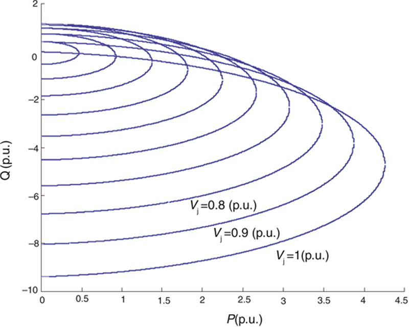
[12] Tachibana M, Palmer MD, Senjyu T, Funabashi T. Voltage stability analysis and (P,Q)–V characteristics of multibus system. CIGRE AORC technical meeting 2014; 2014.

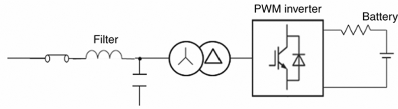
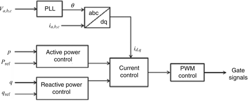
[13] Tachibana M, Palmer MD, Matayoshi H, Senjyu T, Funabashi T. Improvement of power system voltage stability using battery energy storage systems. 2015 International conference on industrial instrumentation and control (ICIC), College of Engineering Pune, India; May 28–30, 2015.

[14] Venkatesh P, Rajendra O, Yesuraj A, Tilak M. Load flow analysis of IEEE14 bus system using MATLAB. Int J Eng Res Technol. 2013;2(5):149155.

[15] Venkatesh B, Rost A, Chang R. Dynamic voltage collapse index – wind generator application. IEEE Trans Power Del. 2007;22(1):9094.

[16] Panov Y, Rajagopalan J, Lee FC. Analysis and design of N paralleled DC-DC converters with master-slave current-sharing control. Applied power electronics conference and exposition, 1997. APEC ’97 conference proceedings 1997, Twelfth Annual, Feb 23–27, 1997, vol.1, 1997. pp. 436–442.

[17] Thottuvelil VJ, Verghese GC. Analysis and control design of paralleled DC/DC converters with current sharing. IEEE Trans Power Electron. 1998;13(4):635644.

[18] Xie X, Yuan S, Zhang J, Qian Z. Analysis and design of N paralleled DC/DC modules with current-sharing control. Power electronics specialists conference, 37th IEEE, June 18–22, 2006. PESC ’06, 2006. pp. 1–4.

[19] Hou D, Liu J, Wang H, Huang W. The stability analysis and determination of multi-module distributed power electronic systems. Power Electronics for Distributed Generation Systems (PEDG), 2010 2nd IEEE international symposium, June 16–18; 2010. pp. 577–583.

[20] Liu F, Liu J, Zhang H. Comprehensive study about stability issues of multi-module distributed system. Proceedings of the 7th international power electronics conference, Hiroshima, Japan; 2014.

[21] Wang H, Liu J, Huang W. Stability prediction based on individual impedance measurement for distributed DC power systems. 2011 IEEE 8th international conference on power electronics – ECCE Asia, Jeju, Korea, May 30–June 03, 2011. pp. 2114–2120.

[22] Liu Z, Liu J, Bao W. A novel stability criterion of AC power system with constant power load. In: Proceedings of 27th annual IEEE applied power electronics conference and exposition; 2012 Orlando, FL, USA. 19461950.

[23] Liu Z, Liu J, Wang H. Output impedance modeling and stability criterion for parallel inverters with average load sharing scheme in AC distributed power system. In: Proceedings of 27th annual IEEE applied power electronics conference and exposition; 2012 Orlando, FL, USA. 19211926.

[24] Liu Z, Liu J, Zhao Y. Output impedance modeling and stability criterion for parallel inverters with master-slave sharing scheme in AC distributed power system. In: Proceedings of 27th annual IEEE applied power electronics conference and exposition; 2012 Orlando, FL, USA. 19071913.

[25] Middlebrook RD. Design techniques for preventing input-filter oscillations in switched-mode regulators. Proceedings of Powercon 5; 1978. pp. A3-1–A3-16.

[26] Suntio T, Leppaaho J, Huusari J, Nousiainen L. Issues on solar-generator interfacing with current-fed MPP-tracking converters. IEEE Trans Power Electron. 2010;25(9):24092419.

[27] Sun J. Impedance-based stability criterion for grid-connected inverters. IEEE Trans Power Electron. 2011;26(11):30753078.

[28] Liu F, Liu J, Zhang B, Zhang H, Hasan SU, Zhou S. Unified stability criterion of bidirectional power flow cascade system. Applied power electronics conference and exposition (APEC), 2013 28th Annual IEEE, March 17–21; 2013. pp. 2618–2623.

[29] Liu F, Liu J, Zhang B, Zhang H, Hasan SU. General impedance/admittance stability criterion for cascade system. ECCE Asia Downunder (ECCE Asia), 2013 IEEE, June 3–6; 2013. pp. 422–428.

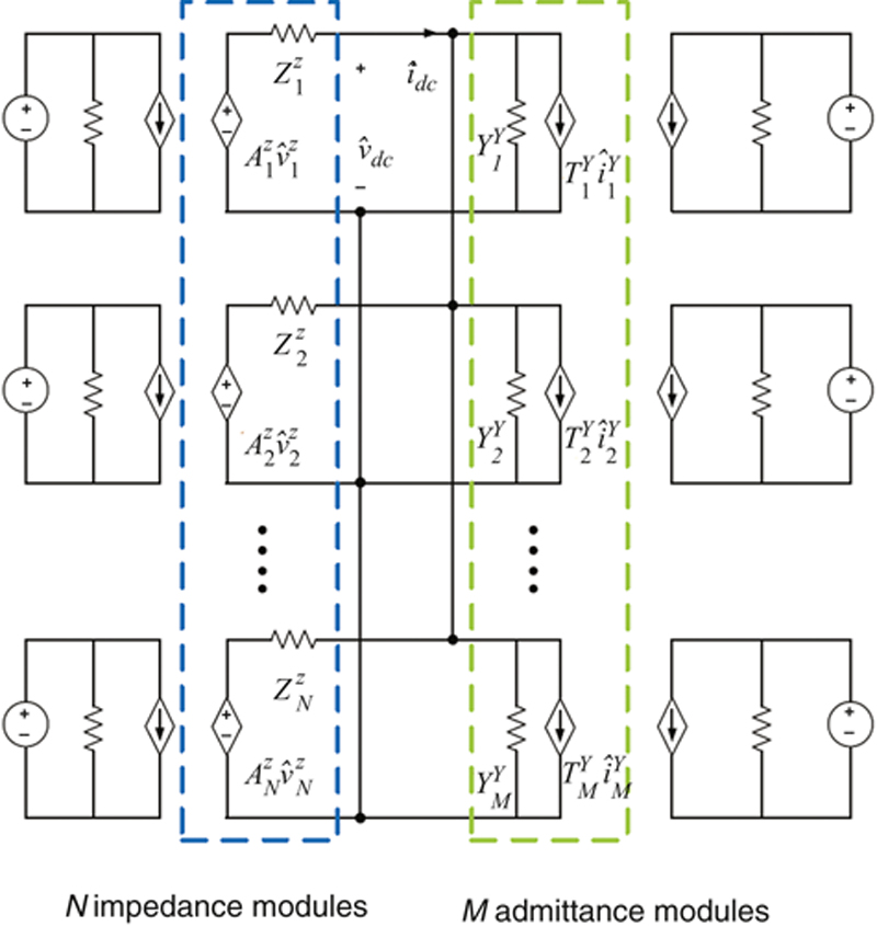
[30] Liu F, Liu J, Zhang H, Xue D. Generalized stability criterion for multi-module distributed DC system. J Power Electron. 2014;14(1).

[31] Liu F, Liu J, Zhang H, Xue D. Terminal admittance based stability criterion for multi-module DC distributed system. Applied power electronics conference and exposition (APEC), 29th Annual IEEE; 2014.

[32] Liu F, Liu J, Zhang H. Comprehensive study about stability issues of multi-module distributed system. In: Proceedings of 7th international power electronics conference; 2012 Hiroshima, Japan.

[33] Liu F, Liu J, Zhang H. Stability issues of Z + Z type cascade system in hybrid energy storage system (HESS). IEEE Trans Power Electron. 2014;29(11).

[34] Liu F, Liu J, Zhang B, Zhang H, Hasan SU, Zhou L. Stability issues of Z + Z or Y + Y type cascade system. Energy conversion congress and exposition (ECCE), 2013 IEEE, September 15–19; 2013. pp. 434, 441.

[35] Schwaegerl C, Tao L. Quantification of technical, economic, environmental and social benefits of microgrid operation, Chapter 7. In: Hatziargyriou N, editor. Microgrids architechtures and control. Chichester, West Sussex, UK: Wiley, IEEE Press; 2014.

[36] Gabbar H, Bower L, Pandya D, Islam F. Resilient micro energy grids with gas-power and renewable technologies, ICPERE, Bali, Indonesia; 2014.

[37] Hojo M, Ikeshita R, Yamanaka K, Ueda Y, Funabashi T. Frequency regulation in a microgrid by voltage phasor regulation of a photovoltaic generation unit, 2015 IEEJ PES – IEEE PES Thailand Joint Symposium, Thailand; 2015.

[38] Ota T, Mizuno K, Yukita K, Nakano H, Goto Y, Ichiyanagi K. Study of load frequency control for a microgrid, power engineering conference, AUPEC 2007, Australasian Universities; 2007.

[39] Sumita J, Nishioka K, Noro Y, Ito Y, Yabuki M, Kawakami N. A verification test result of isolated operation of a microgrid configured with new energy generators and a study of improvement of voltage control, IEEJ Trans, PE, vol. 129. 2009. pp. 57–65 (in Japanese).

[40] Arai J. New inverter control in an isolated microgrid composed of inverter power sources without synchronous generator, IEEE, PES, Thailand Joint Symposium; 2015.

[41] Kasem A, Zeineldin H, Kirtley J. Microgrid stability characterization subsequent to fault-triggered islanding incidents, IEEE Trans, PE, vol. 27. 2012. pp. 658–669.

[42] Noda T, Ametani A. XTAP, chapter 5. Numerical analysis of power system transients and dynamics IET; 2015.

[43] JEAC. Grid-interconnection code, JESC E0019; 2012 (in Japanese).

[44] Takano T, Kojima Y, Temma K, Simomura M. Isolated operation at Hachinohe micro-grid project. IEEJ Trans PE. 2009;129:499506: (in Japanese).

..................Content has been hidden....................

You can't read the all page of ebook, please click here login for view all page.
Reset
3.144.31.163