Chapter 10

AC/DC microgrids

Kazuto Yukita    Aichi Institute of Technology, Department of Electrical Engineering, Toyota, Japan

Abstract

In recent years, the severity of worldwide environmental problems such as global warming and extreme weather events has intensified, while efforts to reduce adverse environmental impacts and to introduce alternative energy sources to replace fossil fuels have been actively promoted. In the field of electrical energy, distributed power sources that utilize natural and renewable energy sources, such as photovoltaic and wind power generation, as well as biomass power generation and fuel cell technology, continue to be active areas of research and development.

Keywords

microgrids
energy
power
photovoltaic
wind
In recent years, the severity of worldwide environmental problems such as global warming and extreme weather events has intensified, while efforts to reduce adverse environmental impacts and to introduce alternative energy sources to replace fossil fuels have been actively promoted. In the field of electrical energy, distributed power sources that utilize natural and renewable energy sources, such as photovoltaic (PV) and wind power generation (WG), as well as biomass power generation and fuel cell technology, continue to be active areas of research and development.
Power generation systems that use natural energy have been highly anticipated; however, with some distributed power sources, it is difficult to achieve stable power generation owing to the dependence of the energy sources on weather and other natural conditions. Thus, research into power supply systems configured from distributed power sources that have already been introduced within specific areas is being actively pursued with the aim of achieving both environmental compatibility and power supply stability. Furthermore, with the widespread popularization of information and communication technology, consumers have adopted stringent requirements with regard to power quality (frequency, voltage, and harmonics).
In this chapter, AC/DC microgrids that have introduced an electrical generating system supplied with renewable energy are described.

10.1. Basic concept of AC microgrids [1]

The concept of the typical AC microgrid is shown in Fig. 10.1. It consists of DGs (PV, WG, FC, etc.), a bidirectional converter, an ACSW, and Valve-Regulated Lead-Acid battery (VRLA) batteries. The bidirectional converter and the DGs are connected to an AC grid, and the ACSW is inserted between the utility and the AC grid. The VRLA batteries are connected through the DC bus to the bidirectional converter. The system changes between each operational mode easily and without any interruptions. The transition of the system is shown in Fig. 10.2. Table 10.1 shows the operational modes. This system has three modes, and their details are explained subsequently. Then, in all modes, the inverter and the converter for DGs are operated using maximum power point tracking.
image
Figure 10.1 Basic concept of AC microgrid.
image
Figure 10.2 State transition diagram of the system

Table 10.1

System Operation Mode

Mode ACSW Bidirectional Converter Operation AC Voltage/Frequency DGs Harmonics
Islanding OFF

Asynchronous operation

Asynchronous AC output with utility grid
Constant Maximum power point tracking (MPPT) Repression of voltage distortion in AC-grid

Synchronous operation

Synchronous AC output with utility grid
N/A
Connected ON
Active filter for harmonics current
Battery charging
Depends on utility grid Repression of harmonic current as AC input
Back up OFF
Asynchronous AC output with utility grid
Constant Repression of voltage distortion in AC grid

10.1.1. Islanding mode

When the system operates in the islanding mode, it is disconnected from the utility grid by turning off the ACSW. The operator then chooses either asynchronous or synchronous operation.

10.1.1.1. Asynchronous operation

The output of a bidirectional converter is a waveform that has constant voltage and constant frequency. The voltage is adjusted so that it does not deviate from the nominal voltage (200 V) by more than 2%, and it also does not deviate from the typical frequency (60 Hz) by more than 0.1%. In this mode, even if the bidirectional converter has a problem, the ACSW will be turned on after an interval.

10.1.1.2. Synchronous operation

The output of a bidirectional converter is a waveform that is synchronous to the utility grid. Voltage amplitude and voltage phase in the AC grid are synchronized with the utility grid. Thus, if the voltage and the phase of the utility grid vary, so do the voltage and the phase of the system. Even though the bidirectional converter may have a problem, the system continues to supply power to the load when in connected mode. When the ACSW are turned on, there is no phase jump.

10.1.2. Connected mode

When the VRLA batteries discharge, the voltage of the DC bus drops to the lowest threshold, and the system starts to charge the VRLA batteries. In that case, the operation mode is changed to the connected mode. In this mode, the thyristors (SCR) serving as ACSW are turned on alternately every half cycle. In the connected mode, the bidirectional converter operates not only as a rectifier for batteries charging but also as an active filter for rejecting harmonic current from loads. When the bidirectional converter charges the VRLA batteries, the bidirectional converter is initially operated by constant current (CC) control. When the DC bus voltage increases to the highest threshold, the system changes to the islanding mode. Furthermore, we can change each value of the current via CC control.

10.1.3. Backup mode

During the charge operation, any problems in the utility grid, for example, a dip in voltage, can turn the ACSW off. Then, the operational mode of bidirectional converter is changed to asynchronous operation of the islanding mode, the system continues to supply power.

10.1.4. Experiment field and device specification

Fig. 10.3 shows the two sets of microgrid systems used in the study. Both systems are almost the same, except for the capacity of the VRLA batteries. One of the systems was set up in Building 12, a building with five floors, with rooms usually used as classrooms and offices. The electric loads are lights and air conditioners. The other system is installed in a library. The library has four floors with book storerooms and reading rooms. The electric loads are lights and PCs. Because 50 kVA transformers were put into the buildings, the capacities of the bidirectional converters were set to 50 kW. We also set up two kinds of PV panels. One of them is a polycrystal silicon type that has a typical output power of 10 kW. The other type is monocrystal silicon, with a voltage of 10 kW. We use VRLA batteries because they are a commonly used energy source.
image
Figure 10.3 AC/DC microgrid systems.

10.1.5. System operation

The load duration curves and frequency distributions of the PVs’ output are shown in Fig. 10.4. The data were collected in May 2008. The data were taken every 5 s for 24 h, that is, at 17,280 points. As shown in Fig. 10.3, the measurement points are “A,” “B,” “C,” and “D.” Points “A” and “C” are outputs of the PVs. Points “B” and “D” are inputs of the loads. We can see that the load consumption of the library is fixed in both operation and nonoperation modes. At Building 12, the connected loads were controlled. Therefore, the total load consumption was smaller than the amount of electric power generated by PV.
imageimage
Figure 10.4 Load duration curve and PV output.
(a) Building 12; (b) library.
However, at the library, the total load consumption is greater than the electric power generated by PV, because the connected loads were not controlled. The power flows in the AC grid of Building 12 (i.e., those of the utility grid), PV output, and load consumption are shown in Fig. 10.5. The utility grid power increased from 5 to 8 am, which indicates the battery charging in the connected mode. Further, the power supplies to loads continued for a whole day, which shows that state migrations were complete.
image
Figure 10.5 Daily load curve of Building 12.

10.1.6. Measurement of power quality

To measure power quality, the PV power is connected through the PV inverter, and the bidirectional converter and ACSW are connected with the AC grid. Further, the VRLA batteries are connected through the DC bus to the bidirectional converter. The loads are the lights and the air conditioners in Building 12. The load power was set in the range from 5 to 8 kW, and the PV output ranged from 2 to 8 kW. The system operated in the islanding and connected modes.

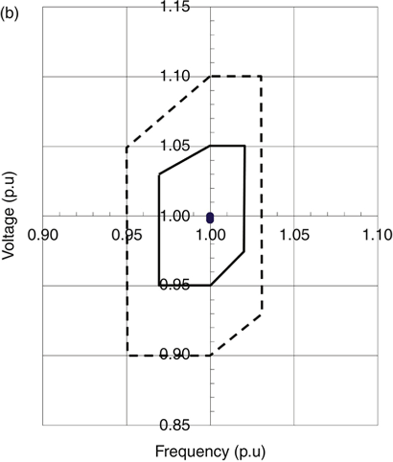
10.1.6.1. Voltage and frequency

The voltage–frequency characteristics are shown in Fig. 10.6 for asynchronous operation and asynchronous operation in the islanding mode. The root mean square (RMS) voltage of the AC grid in Building 12 (Point “F” in Fig. 10.3) is plotted on the vertical axis, and the frequency is plotted on the horizontal axis. In addition, the areas enclosed by the dashed line and the solid line show how much operational voltage is required for the induction motor, written as JEC-2137-2000 in Japanese. The first area shows the short-term operational requirement, and the second shows the long-term operation requirement. Although both modes meet each requirement, in the case of the asynchronous mode, the improved power quality is clear.
imageimage
Figure 10.6 Voltage–Frequency characteristics.
(a) Synchronous; (b) asynchronous. Samples: 14,400 points (for 12 h period in 2008).
10.1.6.1.1. Voltage harmonics
The total harmonic displacement (THD) and the rate of content that is in accordance with the degree of voltage harmonics at the AC grid in Building 12 (Point “F” in Fig. 10.3) is shown in Fig. 10.7. There is a guideline in Japan requiring that the THD of harmonic voltage in a high-voltage line be limited to 5%. Although both operational modes meet this requirement, when the synchronous mode is compared to the asynchronous one, we can see the THD decreases by 0.25% and several higher degrees also decrease. In addition, the cause of the increased 7th harmonics is under investigation.
image
Figure 10.7 Distortion rate and THD of harmonic voltage.
10.1.6.1.2. Current harmonics
The THD and several degrees of harmonic currents, which are the load sides (Point “F” in Fig. 10.3) and the utility-grid sides (Point “E” in Fig. 10.3), are shown in Fig. 10.8. By comparing both sets of data, we can see the effect of using the active filter with a bidirectional converter. As shown in Fig. 10.8, the THD decreases by 1.27%, and there is also a decrease of several higher degrees.
image
Figure 10.8 Distortion rate and THD of harmonic current.

10.2. Battery charge pattern and cost [2]

In this section, we focus on receiving power from the utility grid and study ways to reduce the cost of electricity. When this microgrid system receives power from the utility grid, most of the power is used to charge the battery. Therefore, we tested several patterns for charging the battery and calculated the cost of electricity based on these test results. As a result, we found that when we reduce the peak power and extend the charge times, the cost of electricity is reduced.
Fig. 10.9a details the utility power that is shown in Fig. 10.9b. The AC microgrid system is based on supplying to the load with the minimum utility power necessary. However, it is difficult for the PV system to supply stable power generation to the load. Therefore, in fact, we have relied on receiving power from the utility grid. Table 10.2 shows the average battery charge times from Jan. to Dec. 2008. This table shows that it is charged more than once per day on average. We can see that it is difficult to supply power only by PV generation and the battery. Considering this, our focus was on the economical operation of this system and a reduction of the cost of electricity. In particular, when this system receives power from the utility grid, its purpose is to charge the battery. Therefore, we changed the charge pattern for the battery, focusing on the following.
1. The cost of electricity is decided based on the peak power from the utility grid. We studied charge patterns to reduce the use of peak power.
2. The price of electricity is lower at night than at other times of day. We studied the charge pattern to make maximum use of the night rate.
imageimage
Figure 10.9 Daily power load curve.
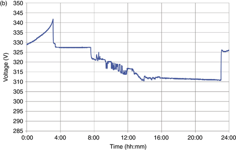
(a) Utility power in a day; (b) power flow and load curve in a day.

Table 10.2

Average Battery Charge Times

Operated Days Charged Times Average Per Day
169 (days) 269 (times) 1.59 times/days
Based on these two points, we supposed that charging the battery is done at the night rate. We also calculated the effect of charge patterns on the cost of electricity used. In practice, because the PV power and load change from day to day, the battery energy does not stay constant.

10.2.1. Battery charge method

The battery is initially charged by constant current (CC) control. Then, the DC bus voltage increases to specified values, and the charge mode automatically changes to constant voltage (CV) control. Taking this into consideration, to reduce the commercial power received, we reduce the CC charge value in CC control. However, if this continues, the amount of battery energy is expected to be insufficient. Therefore, we will make up for the energy shortfall to extend the time of the CV control. To use the night rate more, we set the charge terms of CV control at 8 h. In this test, the charge for the battery is controlled by the bidirectional converter, so we change the setup value. The test results are described further.

10.2.2. Test results

10.2.2.1. Charge pattern

We set the following three cases as charge patterns for the battery. We measured the voltage, current, peak power, and charge energy for the battery.
Pattern (A), CC charge value: 25 A, CV control time: 2 h
Pattern (B), CC charge value: 18 A, CV control time: 2 h
Pattern (C), CC charge value: 25 A, CV control time: 8 h
Fig. 10.10a–c shows the battery voltage and current for the aforementioned patterns.
imageimageimage
Figure 10.10 Current and voltage during battery charge.
(a) CC charge value 25 A, CV charge time 2 h; (b) CC charge value 18 A, CV charge time 2 h; (c) CC charge value 25 A, CV charge time 8 h.
The test circuit was the same as in Fig. 10.3, and the specification was the same as in Table 10.3. The load curve was almost the same as described in Fig. 10.9. The peak demand was about 5 kW.

Table 10.3

Device Specifications

Devices Quantity Capacity Remarks
Photovoltaic (PV) panels 2 10 kW
PV inverter 2 10 kW
PV converter 2 10 kW
Bi-directional converter 2 50 kW
VRLA batteries 2

2V 200Ah

2V 100Ah

168 (cells/set)

10.2.2.2. Test result

Fig. 10.10 shows the period from beginning to measure the data. After 4 hours, the direction of the battery current changes from negative to positive, changing the operating mode of the system from islanding to connected and charging the battery. Immediately after the connected mode starts, the battery begins to be charged by the CC control mode. After the battery voltage approaches a constant value, the charge mode changes to CV control. Furthermore, from the results shown in Fig. 10.10, we could ensure that the system is operated accurately with this CC and CV control mode.
Fig. 10.11 shows a comparison of the charge power of the battery under different circumstances. Fig. 10.11a shows the case of reducing CC value, and Fig. 10.11b shows the case of extending CV terms. Furthermore, the results of calculating electric energy are shown in Table 10.4. From Fig. 10.11, we see the effect of peak power reduction on reducing the CC charge value. We also investigated changing the CV control time from 2–8 hours when the CC charge value was the same. It is clear that the charge power of 8 hours was less than that of 2 hours. As Table 10.4 suggests, when we changed the charge pattern, the charge power required was reduced by 17% from 38.52–31.74 kWh. The reason is thought to be that distinguishing the discharge value before the battery is charged affects the charge power.
imageimage
Figure 10.11 Comparison of the charge power.
(a) The case of reducing CC value; (b) the case of extending CV terms.

Table 10.4

Charge Pattern

CC Charge Value (A) CV Charge Value (h) Peak Power (kW) Electric Energy (kWh)
1 25 2 8.9 38.52
2 18 2 6.27 34.07
3 25 8 9.22 31.74

10.2.2.3. Effect on electric rate

We estimated the cost of electricity for one month based on the test results in the previous paragraph. As a prerequisite for this calculation, the charge power was almost the same the entire time. In this situation, we studied the effect on reducing the cost of electricity used. When we changed the CC charge value arbitrarily, we would also change the CV control time so that the charge power was always kept constant. We used the following conditions to calculate the cost of electricity:
Basic charge = peak power × basic unit price
Energy charge = total charge times × energy unit price (total charge times = CC charge time + CV charge time)
Receiving power is considered to be as follow: 1 day of test data × 30 days
The battery finishes charging at the night rate.
The charge power is constant the entire time. (Prices set by Chubu Electric Power.)
The calculation results are shown in Fig. 10.12. We see that, if we assume that the charge power for the battery is always the same, lengthening the total charge times and lowering the peak power is effective for reducing the cost of electricity. In this system, we changed the total charge times from 4.5–6 hours, reducing the cost of electricity by 10%. It is preferable to charge the battery at the night rate, and it is much better for it to finish charging before the PV generator starts to generate power.
image
Figure 10.12 Effect of charge times on electricity rate.

10.3. Supply and demand control of microgrids [3,4]

The peak cut/peak shift mode operation and the receiving constant power mode operation are described as an example of the control of a supply and use of a demand control in this section.

10.3.1. Peak cut/peak shift mode operation

Fig. 10.13a shows the electricity demand that can be put in the grid using an energy storage system during a peak of electricity demand. Then, Fig. 10.13b shows the relationship between the electricity rate and the charge pattern for the VRLA batteries. It is important to charge the batteries during times when the electricity rate is low and to discharge the batteries during times when the electricity rate is high. In this manner, a reduction in electricity cost can be expected. A concrete instance follows.
image
Figure 10.13 Daily load curve and electricity rate.
(a) Day load curve of the peak cut/peak shift operation; (b) electric rate.
Fig. 10.14 shows the result of the experiment in the case of the peak cut/peak shift for the AC microgrid system. Fig. 10.14a shows the daily load curve. Fig. 10.14b shows the DC voltage curve. Between 8:30 and 15:10, the load was over 5 kW. The maximum receiving power was about 5 kW, and it was confirmed that the system was performing the peak cut operation. The batteries were charged from 23:00 to 24:00 and from 0:00 to 3:10. The batteries made up for a power shortage by discharging when the utility power exceeded 5 kW. It was confirmed that the system performed the peak shift operation. We investigated whether a reduction of electric power cost and a smoothing of the received power occurred by the peak cut/peak shift operation.
imageimage
Figure 10.14 Daily power load curve and DC voltage curve.
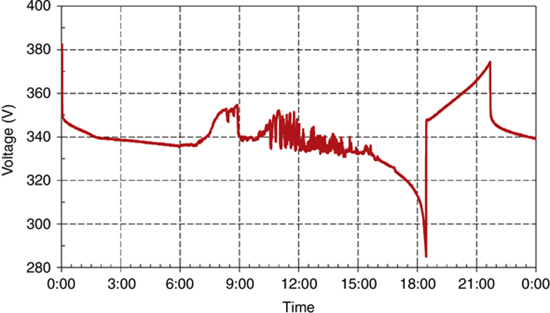
(a) Daily load curve; (b) DC voltage curve.

10.3.2. Receiving constant power mode operation

When the receiving constant power mode operation is put into effect, an adjustment of supply and demand is put into effect by the energy storage system in the microgrid. As a result, influence on the utility power system of the microgrid can be reduced. Predictions of the amount of distributed generation and the electric load power quantity are needed for the implementation of this operation mode. The quantity of constant power received is calculated based on the prediction results.
Fig. 10.15 shows the output of solar power generation and daily load power curve when receiving a constant amount of power from the utility power system. On this day, the predicted amount of PV power was forecast to be insufficient to meet load demand, even though we charged the batteries from 7:00 to 23:00 on the previous day.
image
Figure 10.15 Daily load curve.
Therefore, it was possible to maintain battery capacity while reducing the amount of power received during the day. On this day, the amount of charge and discharge of the battery is a discharge of 8 kWh, the prediction errors are much better than the aforementioned results. Battery voltage on this day is shown in Fig. 10.16. It can be seen that it was possible to maintain the battery voltage between 315 and 335 V.
image
Figure 10.16 Battery voltage.

10.4. Basic concept of DC microgrids

Recently, distributed generation and energy storage technology have become a point of focus for various reasons based on consideration forwards the environment and energy. These technologies can improve energy efficiency of DC loads and electric loads that contain a DC link, such as light-emitting diode (LED) light, LED television, and air conditioning. The use of a DC power supply can be expected to reduce the number of AC/DC converters, as shown in Fig. 10.17. Because a DC distribution grid can do without a DC–AC inverting link in distributed generation, the DC load, power electronic equipment, etc. are merged into the AC grid, with the ability to improve power distribution reliability and power quality.
image
Figure 10.17 AC and DC distributed systems.
Next, we consider the applicability of the DC power supply. There are two types to change electric power in home electric appliances.
Type 1: Equipment with AC motors and heaters, etc.
Type 2: Equipment with a rectifier and an inverter.
Type 1 is suitable for an AC power supply, and Type 2 is feasible by adopting an appropriate direct current voltage, showing the merit of a DC power supply. Therefore, the efficiency improvement when putting a DC power supply into use with equipment that can be put in the home was calculated as a test. Test results of electricity supply efficiency using a direct current electricity supply are shown in Table 10.5. As a result, it seems possible to reduce the power consumption by about 4.7%. The power consumption at home make up about 1/3 of the power consumption in the whole of Japan. By using DC power supply, it expect that power consumption in the whole Japan can be reduced by about 2-3%.

Table 10.5

Calculation Result of the Energy Saving Effect by the Direct Current Electricity Supply [5]

Equipment Number of Units Consumed Power of One (Wh/year) Consumed Power (Wh/year) Amount of Efficient Improvement by the Power Supply Side in DC/AC Reduction (%) Efficiency Ratio of a Household (%)
Air conditioning (2.2 kW) 3 700 2100 3.0 2.66
Refrigerator (500 L) 1 300 300 3.0 0.24
Hot water supply 1 600 600 3.0 0.47
Induction Heating Cooking Heater 1 600 600 3.0 0.57
Microwave 1 70 70
Rice cooker 1 100 100
LED illumination 5 120 480 3.0 0.76
Liquid crystal television (40 in.) 2 150 300
Recorder 1 80 80
Other 1696
Total 6326 4.70

Figs. 10.18 and 10.19 show the main DC microgrid demonstration tests in Japan and the USA. Thus, the DC microgrid experiments aim at a more efficient use of energy.
image
Figure 10.18 Demonstration tests in Japan [6].
image
Figure 10.19 Demonstration tests in the USA [6].

10.4.1. System operation of DC microgrid [7]

Fig. 10.20 shows the configuration of a DC microgrid system. The DC power system consists of PV and WG generation systems, DC/DC converters, a bidirectional converter, storage batteries, DC load, and AC load. The DC power produced by PV and WG generation is connected through a DC/DC converter to the DC bus, and power is supplied through the bidirectional converter to the AC load and the DC load. At this point, if the demand for load power is larger than the amount of power supplied via PV and WG generation, an amount equal to the power shortage is supplied from the storage batteries via the bidirectional converter. If the load power demand is less than the amount of power generated by the PV and WG, the surplus power is used to charge the storage batteries. Furthermore, in situations where the discharge of power from the batteries continues until there is a shortage of stored power, the system transitions to the interconnection mode and the batteries are charged.
image
Figure 10.20 DC microgrid system.
Fig. 10.21 shows the power flow and the load curve data for this system in a day. Fig. 10.22 shows the battery voltage. The horizontal axis is the time of day. The curves show the utility power, PV power, load power, and battery voltage. The main AC load is caused by lighting and an air conditioner. The main DC load is used for the computer servers. In Figs. 10.21 and 10.22, this means that the system is connected to the utility grid. During the hours from 0:00 to 18:30, it is not connected to the utility grid, and the power supply to the load is covered by PV and battery discharge or battery discharge alone. Then, it is proven that there is a correlation between the fluctuation of power variation of the solar PV generation and the output of the converter. In the fluctuation of an output of the converter, this adjusts the balance of power supply and power demand.
image
Figure 10.21 Power flow and load curve in a day.
image
Figure 10.22 Battery voltage in a day.

10.5. Examples of microgrids in the world

A microgrid may also be defined as a self-contained subset of an area electric power system with access to indigenous distributed generation sources, energy storage devices, power loads, and control system. Microgrids possess several advantages, such as the potential for higher power supply availability and security for critical loads, investment deferrals in transmission and centralized generation plants, the provision of ancillary services to a business continuity plan, and opportunities for economic incentives for customers. Therefore, a multilateral match is accomplished throughout the world for microgrids. A typical match is shown in Table 10.6.

Table 10.6

Some Examples of Microgrid Deployments in Different Parts of the World [8]

Location Microgrid
North America Fort Zed, Fort Collins. Colorado; University of San Diego. California; Santa Rita jail, Santa Rita. California; Perfect Power. Chicago, Illinois; BCiT microgrid, Vancouver, BC, Canada; Balls Gap Station, Milton, West Virginia
South America Robinson Crusoe Island, Chile; OHagUe’s microgrid, Chile; Huatacondo’s microgrid. Chile
Europe Model City of Manheim, Germany; Cell Controller Project, Denmark; CRES-Gaidouromanlra, Kythnos, Greece; Liandcr’s Holiday Park at Bronsbcrgen, Zuiphcn, The Netherlands; RSE-DER test facility. Italy; TECNALIA-DRR test facility. Bilbao, Spain; PIME’S project. Dale. Norway; Szentendre, Hungary; Salburua. Spain; La Graciosa Island microgrid, Spain; Optimagrid, Spain; iSare project, Guipiizcoa, Spain
Asia Rural PV hybrid microgrid. West Bank; Hangzhou Dianzi University, China; NbDO microgrid. Aichi, Kyotang, Elaciiinohc. Japan; NEDO Tohoku Fukushi University, Sendai. Japan; Shimi/u Corp. microgrid. Tokyo Gas microgrid, Aiclii Institute of Technology microgrid, Japan; INER microgrid, Taiwan
Africa Diakha Madina, Senegal
Australia CSIRO. Kings Canyon, Coral Bay, Brcmer Bay, Denhem, Esperence, Hopctoun, King Island, Roltnest Island

Note: Information from the US Department of Energy Renewable and Distributed Systems Integration projects and C1GRE WGC6.ll.

10.6. Conclusions

In this chapter, exchange electricity supply and DC electricity supply were explained along with the microgrid, which is a small-scale utility grid into which renewable energy has been introduced. I hope that the use of AC/DC microgrid systems will become increase in future.

References

[1] Takashi T, Keiichi H, Yoshiaki O, Kazuto Y, Ichiyanagi K. Development of uninterruptible power supply system with distributed generators (DGs). INTELEC. 2008;30:574578.

[2] Murai H, Takeda T, Hirose K, Okui Y, Iwase Y, Yukita K, Ichiyanagi K. A study on charge patterns for uninterruptible power supply system with distributed generators. INTELEC. 2009;31:534538.

[3] Hiroaki M, Takashi T, Kazuto Y, Hiroshi M. Comparative study of peak cut/peak shift operation using microgrid. ICEE. 2014; SPGP-2357.

[4] Tomoki K, Kazuto Y, Yasuyuki G, Katsuhiro I, Tomohito U, Keiichi H, Yoshiaki O. Operation method of micro grid using the forecasting method by neural network. ISAP 2013;929

[5] Hiroshi K. Technology and problem of direct current power supply in the home using the 300 voltage. EMC 2013; 2.5(298): 25–38 (in Japanese).

[6] Kazuto Y, Takashi T. Technical trends on the development of DC power system. IEEJ. 2015;135(6):366369.

[7] Yukita K, Shimizu Y, Goto Y, Yoda M, Ueda A, Ichiyanagi K, Hirose K, Takeda T, Ota T, Okui Y, Takabayashi H. Study of AC/DC power supply system with DGs using parallel processing method. IPEC. 2010;(22A2–3):722725.

[8] Abbey C, Cornforth D, Hatziargyriou N, Hirose K, Kwasinski A, Kyriakides E, Platt G, Reyes L, Suryanarayanan S. Powering through the storm: microgrids operation for more efficient disaster recovery. IEEE Power Energy Mag. 2014;12(3):6776.

..................Content has been hidden....................

You can't read the all page of ebook, please click here login for view all page.
Reset
3.15.226.120