
Chapter 3
Operational aspects of distribution systems with massive DER penetrations
Tomonobu Senjyu*
Abstract
Distributed generators (DGs) encompass a huge economical and environmental potential, especially if these DGs are based on renewable energy sources. However, high penetration of DGs into distribution systems can trigger voltage deviations beyond the statutory range, and can reverse power flow toward the substation transformer. Consequently, DGs can increase energy losses if they are not well controlled. Coincidentally, the demand of plug-in electric vehicles (PEVs) is increasing and PEVs will be well spread in distribution systems in the near future. Thus, the aggregated power of the PEVs will play an important role in the power system. However, the mismanagement of this potential power may cause serious losses. Thus, a power scheduling method of photovoltaics (PVs), PEVs, and tap transformers is proposed in this chapter to reduce the total energy losses in the distribution systems. In order to achieve the lowest possible total loss, reconfiguration of the distribution system is considered within every hour at the optimization. In order to show the effectiveness of the proposed method, 1 day ahead power and configuration schedules are generated by using the particle swarm optimization which are based on the weather and load demand predictions. The total expected energy loss from the optimal schedule by considering the system reconfiguration is compared to other losses which are obtained from optimal schedules for different fixed configurations. Other important objectives are also considered such as keeping the voltage within the statutory range and the prevention of reverse power flow to protect the substation transformer.
Keywords
voltage control
distribution system
distributed generator
battery energy storage system
interconnection point power flow
electric vehicle
3.1. Introduction
World primary energy consumption enlarged by 2.3% in 2013, an acceleration of over 2012 (+1.8%). Conventional fossil fuels such as coal, oil, and gas remain the largest sources of world energy. Oil, coal, and natural gas supply the 32.9, 30.1, and 23.7% of global energy consumption, respectively. Unreliable nuclear power provides 4.4% of global energy consumption, and hydroelectric contributes for 6.7% of global energy consumption. The green renewable energy sources deliver a record 2.7% of global energy consumption [1]. According to the BP Energy Outlook 2035, the world’s population is expected to reach 8.7 billion which means an additional 1.6 billion people will require energy. Primary energy consumption of the world will be increased by 37% between 2013 and 2035, with averaging 1.4% per annum (p.a.) growth rate. Therefore, energy production will increase at 1.4% p.a. from 2013 to 2035, matching the expansion of energy consumption. Fossil fuels in cumulative lose share but remain the dominant form of energy in 2035 with a share of 81%, down from 86% in 2013. Renewable energies (eg, wind, solar, tide, biofuel) gain share rapidly, from around 3% today to 8% by 2035, overtaking nuclear in the early 2020s and hydro in the early 2030s. Total carbon emissions from energy consumption will rise by 25% between 2013 and 2035 (1% p.a.), with the rate of growth declining from 2.5% over the past decade to 0.7% [2].
Renewable energies are expected to play a vital role for the reduction of emission and to meet the future energy demand [3]. High penetration of renewable energy sources is required to integrate with the existing power grid. Therefore, the conventional power grid has to be reconfigured for the integration of renewable sources. The reconfiguration form of the existing power grid with renewables is known as the smart grid (SG). Distributed generations (DGs) will play an important role for the future SG [4,5]. DGs consist of wind generator, PV generator, fuel cell, biofuel, smart house, electric vehicle, battery energy storage system (BESS), and so on and are sources of energy which can transport a variety of benefits including improved reliability if they are operated properly by the SG [6]. Furthermore, DGs are energy cost saving [7]. In addition, DGs can improve power system efficiency as well as prosper the power quality of the distribution network [8]. Generation of most DGs mainly depends on the weather conditions. When a large number of DGs are integrated with the power system, there are adverse effects such as power fluctuation, voltage flicker inside the power grid, frequency deviation, energy losses, and so on. Sometimes these problems become severe which cannot be solved by only the tap changing of a load ratio control transformer (LRT) in the substation and step voltage regulators (SVRs) in the distribution line.
To solve that, some control methodologies, which mainly use reactive power controllers such as additional reactive power compensators [9–10] or the reactive power control of DGs [11–12], have been proposed in some literatures. However, these control methods are subject to the power factor control of DGs in spite of being a detriment to the DGs operators by causing a reduction in the active output power. On the other hand, interfaced inverters which are used for variable speed wind turbines and PV generators can control the reactive output power independently within their capacity [13]. Furthermore, a BESS is introduced to the power system to compensate the power quality loss, voltage, and frequency fluctuations [14–16]. In recent years, BESS technologies have been developed to achieve cost reduction, longer operating life, and higher efficiency [17,18]. Therefore, introducing a BESS into the power distribution systems may help to solve some problems caused by a large-scale integration of DGs, based on renewable energies and to achieve some economic operation goals. Centralized control methods and decentralized autonomous control methods have been proposed [19,20] which use the reactive power control function of PV generators. However, in these works, reverse power flows occur at daytime when the output power is large. In addition, interconnection power flow fluctuates considerably, which has a harmful effect for the operation of the modern SG systems.
In the next few years, due to the commercialization of PEVs, an expansion in high market shares is expected [21,22]. The overall fuel conversion efficiency of PEVs is approximately at 22.5–45%, while that of conventional vehicles is estimated at only about 20% [23]. PEVs are environmental friendly because they emit no tailpipe pollutants. With PEVs, electric motors provide quiet, smooth operation and stronger acceleration and require less maintenance than internal combustion engines [24]. Another beneficial feature of the PEVs is that they can perform charge and discharge operations while connected to the home. Therefore, it can be considered as a controllable load, and the use of the PEV as the controller of distribution systems is expected. Another way to reduce distribution losses is to reconfigure the distribution system using electromagnetic switches between specific buses. Much research has been conducted on the optimal network reconfiguration problem for the power loss reduction [25]. Some studies have focused on the loss reduction using only the reconfiguration of the system, some of them have been considered the existence of tap transformers, and others have been taken DGs into consideration. However, none of the studies has combined the usage of PVs, BESS, PEVs, and tap transformers together with reconfiguration for reducing distribution losses. Thus, this problem is addressed in this chapter. It is formulated as an optimization problem and solved to find the best feeder configuration and power references of PVs, PEVs, and tap transformer positions in order to reduce distribution losses of DGs for the SG applications.
3.2. Control objectives
Nowadays, electric power grids are slowly getting smarter. The use of DGs is increasing in the modern power grid. Though SG promoters tout the ability of a smarter grid to enable greater consumption of DGs, the benefits could flow in both directions [26]. A zero emission-based smart DG system is shown in Fig. 3.1. From this figure, all renewable sources, that is, wind farm, PV, smart houses, electric vehicles, and energy storage are connected in a power network which are controlled by an intelligence power controller.

Figure 3.1 A zero emission-based smart distributed system.
3.2.1. Importance of distributed generations
The conventional power generation system depends on the centralized generation system but there are numerous benefits of DGs. The benefits of DGs are as follows [27,28]:
▪ Reduction the transmission loss. Usually, the DGs are located near the demand side. Therefore, they can avoid the expensive and inefficient long-distance transmission of power. A strong power grid is required to transmit power where it is consumed. Installation and maintenance costs of the power grid are expensive. On the other hand, long-distance energy transmission is inefficient due to the transmission loss. Generation and distribution in the locally can improve the power system efficiency.
▪ Lessening peak load demand. Due to the generation in the consumer-side, the DGs can decrease peak demand of a power network. It is an effective solution of the problem of high peak load shortages.
▪ Impacts on local economics and communities. DGs generate clean power locally, which creates job opportunities within the local community. Usually, DGs provide more job opportunities than developing traditional, centralized power stations. DGs can develop within underused spaces such as parking lots, unused fields, and rooftops. Therefore, they do not require the cost involved in building large power plants on undeveloped land. Also, DGs can play an important role to supply power for remote and inaccessible areas which develops the economy of remote communities. In addition, smart houses are gaining interest as a DG. The house receives power from the power grid when generation is lower than the load demand. On the other hand, the house can transmit power to the power grid when generation is more than the load demand. As a result, a house owner can be benefited to sale extra power to the power company.
▪ Faster response to new power demands. The centralized power plant requires a long installation time to deliver power for new demands. However, DGs are small scaled and often require lower installation period, it enables faster response when additional power demands are required.
▪ Improvement of energy security. DGs provide more energy security than the large centralized power plants in case of severe weather condition, natural disasters, human error, and acts of terrorism. If the centralized power plants collapsed, a huge blackout may occur in the large residential area and it becomes disaster for the residents. For example, following an earthquake, tsunami, and the failure of cooling systems at Fukushima I Nuclear Power Plant and issues concerning other nuclear facilities in Japan on March 11, 2011, a huge blackout occurred for a long period of time. A nuclear emergency had been declared in Japan and 140 thousand residents within 20 km (12 mi) of the plant were vacated [29,30].
▪ Improved supply reliability and power management. Each DG of the power system is controlled by the independence utility of grid system which offers easy maintenance of power, voltage, and frequency. It also provides the possibility of combining energy storage and management systems, with reduced obstruction.
▪ Enhancement of the power system. An intelligent grid can support high levels of renewable energy, reducing our dependence on fossil fuels which also reduces emissions of greenhouse gases. A modern power grid incorporating with clean local energy that can fully support electric vehicles which can reduce the reliance on foreign oil.
3.2.2. Challenges of distributed generations system
Conventionally, power generation, transmission, distribution, and load demands have been managed as independent processes. Due to the large amount of DGs in the power network, the traditional approach of the power system management has gradually been shifting [31]. DGs are a vital part of the modern smart power system but integration of DGs in the conventional power network is challenging for the power system engineers. The following are issues regarding the DGs network:
▪ High renewable energy penetration. Renewable energy resources are considered as power generation sources of DGs. Because of high penetration of renewable energy resources in DGs network, active energy resources such as loads, storages, and electric vehicles will be increased. Integration of active power resources into the DGs increases the complexity of power system. Furthermore, generation of renewable sources depends on the weather condition. Power fluctuation from the renewable energy sources is serious concern for the DG networks because it may create frequency deviations, voltage flicker inside the power grid, and power system instability [32–35]. Research has been conducted in order to resolve this problem using energy storage devices [36–40]. However, installation and maintenance costs of energy storage devices are high. If power fluctuation of the DGs is increased, the capacity of the energy storage devices will be increased. Power fluctuations of some DG networks are very high and sometimes it is very difficult to install a large capacity of energy storage in power networks.
▪ Power balancing. DGs may offer operational challenges for a power system. The irregular natural power sources such as wind power and solar always provide a variable energy supply with both predictable (day–night and seasonal) fluctuations and unpredictable fluctuations driven by medium-term weather conditions and forecast errors. Such power fluctuations will require complex power-balancing mechanisms between demand and supply. Hence, alternative power capacities such as conventional generation and energy storage are used to fill up demand/supply gaps when production from renewables is low and high.
▪ Power losses. DGs such as wind farms and PV may be located far from the demand side which requires a long transmission line to deliver the electric power. It may increase the system costs and transmission losses.
▪ Impacts of real-time power market. Many electrical sources have been taken over by independent power producers. This trend leads to the competition in power trades and power sectors [41,42]. Therefore, electricity producers should use conventional fossil fuels based power units efficiently so that they can reduce the operational cost and maximize the profit. Optimum operation of conventional units incorporated with DGs is an important issue for the SG system. Hence, unit commitment programs are introduced in order to deliver the optimum operation of the smart power system [43–47]. On the other hand, power-forecasting error of the DGs system is challenging for the real-time power market. It may increase the energy price of the power company. A reconfiguration or replanning approach of the power system can lessen the forecasting error and expansion the benefits of the power company.
3.2.3. Overview of control system
The objective of this chapter is to perform cooperative control between existing voltage control devices such as LRTs and SVRs, PVs, and BESSs introduced to interconnection points and at the part of a distribution system where it is assumed to have important loads. The proposed method aims to achieve voltage regulation within the acceptable range, smooth the power flow at the interconnection point, to ensure output power if a power outage occurs, and to reduce the total distribution losses.
According to the Electricity Law in Japan, the statutory range of voltage at the residential consumer side must be within 101 ± 6 V. In the distribution systems, between pole transformers, for the 6.6 kV high-voltage distribution system, and on the consumer side, for the 100 V system, when the load is heavy, it can cause up to the 6.5 V voltage drop and flow in reverse. Also, when the power flows to the system from distributed generators (DGs), it can cause up to 2 V voltage rise [48]. Thus, the range of voltage at the residential consumer side is from 101.5 V (0.967 pu) to 105 V (1.0 pu). If all pole transformers are setup at 6.6 kV:105 V, the system should maintain the voltage range within 6.380 kV (0.967 pu) to 6.6 kV (1.0 pu), that is, the high-voltage distribution system. This is the defined acceptable voltage range in this chapter.
In order to smooth interconnection point power flow and to increase the flexibility in the distribution system operation, a bandwidth is defined. In this research, the bandwidth of the interconnection point active power flow is defined as ±0.1 pu (500 kW) from the average of a daily load curve, and the interconnection point reactive power flow range is defined to keep the power factor between 0.8 and 1.0. The interconnection point power flow is controlled by the BESS introduced at that point.
Therefore, the purpose of this research is to maintain the node voltages within the acceptable range which is defined previously, reduce total distribution losses, and interconnect point power flow smoothing.
3.3. Control method
The following section describes the decision technique for the tap changing of existing voltage control devices, and the reactive power control method, using inverters interfaced with PVs, BESSs, and PEVs.
3.3.1. The objective function and constraints
The objective function is used to minimize distribution losses in terms of the node voltages, the tap positions and the reactive output power of the inverters interfaced with PV and BESS. It can be formulated as follows:
3.3.1.1. Objective function
 (3.1)
(3.1)3.3.1.2. Constraints
These constraints are the voltage constraints in the distribution system, active power flow constraints, and reactive power flow constraints, respectively. The bandwidth of voltage and active power flow are already mentioned. The reactive power flow bandwidth is as follows.
 (3.8)
(3.8)
These constraints are the large capacity BESS inverter constraints, considering the loss in charging and discharging of the BESS for each power constraint, and state of charge (SOC) constraints for the purpose of rapid degradation control of the BESS, respectively.
 (3.13)
These constraints are the PV inverter capacity constraints, PEV inverter constraints, SOC of the PEV constraints, and tap transformer’s tap position constraints, respectively. The symbols of the aforementioned equations indicate as follows:
| P B | Active power of the battery |
| Q B | Reactive power of the battery |
| P PV | Active power of the PV |
| Q PV | Reactive power of the PV |
| P EV | Active power of the PEV |
| Q EV | Reactive power of the PEV |
| T K | Tap position |
|
|
Minimum tap position |
|
|
Maximum tap position |
| P L | Total power flow to the distribution network |
| V i | Node voltage |
| V i_min | Minimum node voltage |
| V i_max | Maximum node voltage |
| P f | Active power flow to the interconnection point |
|
|
Minimum active power flow to the interconnection point |
|
|
Maximum active power flow to the interconnection point |
| Q f | Reactive power flow to the interconnection point |
|
|
Minimum reactive power flow to the interconnection point |
|
|
Maximum reactive power flow to the interconnection point |
| S B | Marginal capacity of the inverter for BESS |
| ζ B | SOC of the battery |
| ζ EV | SOC of the PEV |
| S PV | Marginal capacity of the inverter for PV |
| S EV | Marginal capacity of the inverter for PEV |
| η | Efficiency of the system |

3.4. Particle swarm optimization
There are many methods to solve the aforementioned optimization problem. In this work, particle swarm optimization (PSO) [49,50] was chosen. PSO is an optimization method which uses the general idea that a flock of birds can find the path to food by cooperation. This is modeled by the particle swarm which has the search position and velocity information in multidimensional space. The PSO algorithm is follows:
| Step 1 | Generate an initial searching point for each swarm. |
| Step 2 | Evaluate the objective function using each swarm’s searching point. |
| Step 3 | Finish searching if stopping conditions are satisfied. If not, go to Step4. |
| Step 4 | Search the next point considering the best of the current swarm’s searching point and every swarm’s best searching point. Go to Step2. |
The searching algorithm communicates the best positions information to all swarms, and each continues updating their own positions and velocities until finished searching. The updating of velocity and search position is decided by following equation:
where,
| V k+1 (i) | ith particle velocity in k + 1th search |
| rand 1 | Uniform random numbers from 0 to 1 |
| S k+1 | Search position of ith particle in kth search |
| w | Weighting of inertia |
| c 1 | Weighting for best position of self particle |
| c 2 | Weighting for best position of particle swarm |
| pbest | Best position of self particle |
| gbest | Best position of particle swarm. |
3.4.1. PV generator system
In this chapter, the DGs are considered based on PV generators which are becoming more popular in smart houses. The reactive output power from the inverters interfaced to the DGs is used to control the distribution system voltage. The reactive power is maintained within the capacity of the DG inverters while maximizing the PV active power. The reactive power control system scheme is shown in Fig. 3.2. The active power, PPV, from the PV feeds to the maximum power point tracking (MPPT) control system to generate the maximum output power [51]. Then, the output power range is generated from the active power of the PV generator, PPV. It determines the margin of the inverter capacity, SPV. The optimal scheduling reactive power reference, Q*PV adapts the range of the reactive power for the PV generator. The active and reactive powers of the PV generator are estimated the dq to abc conversion [52]. The three-phase voltage reference (abc) is the input of a voltage source inverter, and the inverter delivers the active PPV and reactive power QPV to the distribution networks.

Figure 3.2 Reactive power control system for the PV.
3.4.2. BESS at the interconnection point
To suppress large variations of power flow at the interconnection point, the active and reactive powers are controlled using the BESS at the interconnection point. Fig. 3.3 shows the active and reactive powers control systems of the BESS. The control strategy of the BESS system is similar as the PV system.

Figure 3.3 BESS control system.
In this control system, active power reference signal P*B and the reactive power reference signal Q*B are used for the optimal schedule algorithm. Based on the control references, the PSO-based optimization method considering the forecast information of the BESS is controlled to satisfy the power flow bandwidth constraints at the interconnection point. In this chapter, the BESS is assumed to have a sodium–sulfur battery, and the efficiency of the BESS is 80% without considering self-discharging of the BESS.
3.4.3. Plug-in electric vehicle
The PEV assumed in this chapter is based on commercial PEVs, and the parameters are described in Table 3.1. When the PEV is connected to the grid, we can control the active and reactive powers of the grid. In addition, this chapter considers two different demand areas. Moreover, when the PEV is connected to the grid, the SOC of the PEV corresponding to each area has been taken into consideration. The PEV’s SOC are assumed with a percentage of ownership in a residential area of 80%, and office area of 30%. To cope with the reverse power flow, PEVs are charging in daytime and discharging at nighttime.
Table 3.1
Parameters of the Distribution System
| Parameter | Comparison Method | Proposed Method |
| Line impedance of each section | 0.04 + j0.04 pu | |
| Rated capacity of PV node | 0.08 pu (400 kW) | |
| Rated capacity interfaced inverter of PV | 0.08 pu (400 kW) | |
| Large BESS capacity | 5.0 pu (25 MWh) | 2.0 pu (10 MWh) |
| Rated capacity interfaced inverter of BESS | 0.4 pu (2 MW) | 0.03 pu (1.5 MW) |
| PEV capacity | 0.24 pu (1200 kW) | |
| Rated capacity interfaced inverter of PEV | 0.06 pu (300 kW) | |

3.5. Simulation results
In this chapter, in order to show the effectiveness of the proposed cooperative control method based on optimal reference control, simulations are performed based on the distribution system model which is shown in Fig. 3.4. The system consists of total 15 DGs nodes at two different areas (ie, residential and office areas). In DGs, all nodes are connected to the PEVs and 10 nodes are connected to the PVs (circles indicate of these nodes). Due to the electromagnetic contactor in Fig. 3.4, the distribution systems can be considered as the reconfigurable distribution systems. Line impedances, power factor of the load demand, rated capacity of the inverters interfaced PVs, BESSs, and rated capacity of PEVs for DGs are listed in Table 3.1, where the nominal capacity of the DG and the nominal voltage are 5 MVA and 6.6 kV, respectively.

Figure 3.4 Model of distribution system.
MC, Magnetic connector.
MC, Magnetic connector.
This research assumes to get the high accuracy forecast information of the PV output power and load demand for the next day. The actual PV output power profile for an hour average value is shown in Fig. 3.5a. This power profile has been used for the optimum scheduling method. The load demand profile of a day is shown in Fig. 3.5b, and it is assumed that nodes 11–24 are considered for residential area, while nodes 31–35 are considered for the office area.
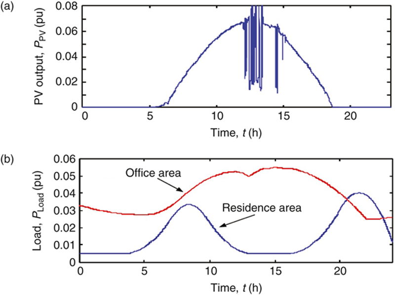
Figure 3.5 (a) PV output power, (b) load demand.
The proposed system (Fig. 3.4) is a reconfigurable distribution system, thus, the distributions can consider for eight cases. The configuration and optimized distribution loss for the 24-h of each case are listed in Table 3.2. It is confirmed from the Table 3.2, that case 2 contains the smallest distribution loss (1469 kWh) among the all cases. Therefore, case 2 is selected for the comparison method. The comparison method considers the optimize approach where the distribution loss is the smallest. Finally, the proposed method considers the 1-h optimization for all cases. After comparing the all cases results, the proposed method selects the best case where the distribution loss is minimal. This action repeats for 24 h.
Table 3.2
Distribution Loss of Each Case
| Case | Close EC | Distribution Loss (kWh) | Case | Close EC | Distribution Loss (kWh) |
| 1 | 1,2,3 | 1541 | 5 | 1,2,5 | 1910 |
| 2 | 2,3,4 | 1469 | 6 | 1,3,4 | 2920 |
| 3 | 2,3,6 | 1451 | 7 | 1,4,5 | 2422 |
| 4 | 1,2,6 | 1757 | 8 | 1,3,6 | 2242 |

Table 3.3 shows the selected case for every hour of the proposed method. From this table, case 1 and case 3 are selected relatively more than other cases. However, there is a very important matter to select case 8 at time 10–18 h. The reason behind this is that all DGs are connected in series for case 8. Usually, in that time, the output power of the PV is maximum, and it is difficult to reduce the distribution loss of the system. Since, the DGs are connected in series for case 8, it is more flexible for the voltage control using the reactive power control from these DGs. From Table 3.3, the distribution loss of the proposed method (1129 kWh) is smaller than the comparison method (1469 kWh). The simulations have been conducted in three patterns as follows: without optimization method (ie, without any control devices), comparison method, and proposed method. The dynamic responses of each method are described in the following subsection.
Table 3.3
Results of the Proposed Method
| Time | 1 | 2 | 3 | 4 | 5 | 6 | 7 | 8 | 9 | 10 | 11 | 12 |
| Case | 3 | 3 | 1 | 1 | 1 | 2 | 1 | 1 | 4 | 3 | 7 | 8 |
| Time | 13 | 14 | 15 | 16 | 17 | 18 | 19 | 20 | 21 | 22 | 23 | 24 |
| Case | 8 | 8 | 8 | 3 | 3 | 3 | 3 | 3 | 1 | 3 | 1 | 1 |
| Distribution loss | 1129 kWh | |||||||||||

3.5.1. Dynamic responses for the without optimization approach
Simulation results for the without optimization method are shown in Fig. 3.6. Fig. 3.6a shows the node voltages of the distribution system, where the dashed lines indicate the acceptable voltage range or constraint of the node voltages. From this figure, the acceptable range of the node voltages is very narrow and fluctuates over the acceptable range. Therefore, the without optimization approach cannot control the node voltages and the system may fall into an imbalance situation. From Fig. 3.6b–c, active and reactive powers of the system are also fluctuated over the acceptable ranges. Therefore, the without optimization method cannot control the system appropriately.

Figure 3.6 Simulation results of without optimization control.
(a) Node voltages, (b) active power flow at interconnection point, and (c) reactive power flow at interconnection point.
(a) Node voltages, (b) active power flow at interconnection point, and (c) reactive power flow at interconnection point.
3.5.2. Dynamic responses for the comparison method
Simulation results of the comparison method are shown in Fig. 3.7. The dashed lines of these figures mean the acceptable range or constraint of the system. Fig. 3.7a shows the node voltages of the comparison method. From this figure, the node voltages satisfy the constraint of the system, and due to the active output powers of the PV generators, the node voltages are high at the time 10–18 h. If the lower-node voltages are required at this time, the distribution must be controlled by the active powers of the PV generators. The active and reactive powers at the interconnection point are shown in Fig. 3.7b–c, respectively. Both figures also fulfill the constraints. Again, from Fig. 3.7b, the active power flow is always in the lower acceptable range. It means that the active power flow satisfies the constraint even if the acceptable range is lower. The dashed lines in Fig. 3.7c are always a constant value because the active power flow is almost constant at every time.


Figure 3.7 Simulation results of the comparison method.
(a) Node voltages, (b) active power flow at interconnection point, (c) reactive power flow at interconnection point, (d) active and reactive output powers from BESS, (e) state of charge of the BESS, (f) active and reactive output powers of PEV at residence area, (g) active and reactive output powers of PEV at office area, (h) state of charge each area of PEV, (i) reactive output power of the interfaced DGs, and (j) tap positions.
(a) Node voltages, (b) active power flow at interconnection point, (c) reactive power flow at interconnection point, (d) active and reactive output powers from BESS, (e) state of charge of the BESS, (f) active and reactive output powers of PEV at residence area, (g) active and reactive output powers of PEV at office area, (h) state of charge each area of PEV, (i) reactive output power of the interfaced DGs, and (j) tap positions.
The active and reactive powers of the BESS are depicted in Fig. 3.7d. Most of the time, the active power is larger than the reactive power of the battery. Therefore, it can confirm that the main work of the BESS is the active power control at the interconnection point. At the time 10–18 h, the active power of the battery is negative (which means battery is charging at this period) because the generation of the PV is high in this period. The SOC of the BESS is indicated in Fig. 3.7e. From this figure, the SOC satisfies the constraint of the BESS. Therefore, it is possible to construct a stable charge and discharge actions of the BESS. Figs. 3.7f–g show the active and reactive powers from the PEV at residence and office areas, respectively. It is confirmed that the reactive power is higher than the active power in both areas. It means the voltage control by the reactive power is more effective than the active power control to improve the distribution qualities.
The SOC of each PEV is shown in Fig. 3.7h. It can be seen from this figure, the SOC of each area is almost same. Therefore, it reflects that the SOC of the PEV is in balance at each area. Fig. 3.7i shows the reactive output power from the PV generator. The reactive output power is positive for the voltage enlargement. The tap positions of LRT and SVRs are depicted in Fig. 3.7j. The limit of the tap position is defined as 0.90 ≤ Tk ≤ 1.10. From Fig. 3.7j, the tap position can be controlled within constraints. From the comparison method, the voltage control is accomplished by the reactive power from PV and PEV, and power flow control is achieved by the active power control of the BESS.
3.5.3. Dynamic responses for the proposed method
Fig. 3.8 shows the simulation results for the proposed method. The constraints of the proposed method are followed as similar as the comparison method (Fig. 3.7). In spite of the same SOC of the PEV (Figs. 3.8h and 3.7h) in both methods, the SOC of the BESS for the proposed method in Fig. 3.8e is around 10% higher than the comparison method (Fig. 3.7e). Therefore, it is confirmed that the proposed method can reserve the energy of the BESS.


Figure 3.8 Simulation results of the proposed method.
(a) Node voltages, (b) active power flow at interconnection point, (c) reactive power flow at interconnection point, (d) active and reactive output powers from BESS, (e) state of charge of the BESS, (f) active and reactive output powers of PEV at residence area, (g) active and reactive output powers of PEV at office area, (h) state of charge each area of PEV, (i) reactive output power of the interfaced DGs, and (j) tap positions.
(a) Node voltages, (b) active power flow at interconnection point, (c) reactive power flow at interconnection point, (d) active and reactive output powers from BESS, (e) state of charge of the BESS, (f) active and reactive output powers of PEV at residence area, (g) active and reactive output powers of PEV at office area, (h) state of charge each area of PEV, (i) reactive output power of the interfaced DGs, and (j) tap positions.
3.6. Conclusions
This chapter analyses an optimal control method of PV interfaced inverters, LRTs and SVRs, house BESSs, large BESSs, and PEVs in reconfigurable distribution systems. This chapter also introduces distributed energy sources, energy storages, and SG application. From the simulations, it is confirmed that the proposed method can reduce the distribution losses as compared with the comparison method. The reference schedule is optimized based on constraints of these control devices. Comparisons of the results are analyses in different cases. The distributed energy sources are an important element of the SG systems. Therefore, analyses of this chapter are effective to reduce the overall losses for the SG systems.
..................Content has been hidden....................
You can't read the all page of ebook, please click here login for view all page.