4 FEM Analysis

Search in book...
Toggle Font Controls
Create new playlist

Name your new playlist

Playlist description (optional)
Sign In

Email address

Password

Forgot Password?

or

Continue with Facebook

Continue with Google
Sign Up

Full Name

Email address

Confirm Email Address

Password

or

Continue with Facebook

Continue with Google

Linear-motion electromagnetic systems have been widely studied using electric circuit approach, e.g., [24, 63, 71, 142, 160]. Their operation can be simulated more accurately on the basis of electromagnetic field analysis [48, 101, 173]. Accurate estimation of electromagnetic parameters is very important. The inductance of the stator windings and the propulsion force (thrust) can be calculated from the field differential parameters such as magnetic potential and magnetic flux density distributions.

The finite element method (FEM) analysis allows for calculating the magnetic field distribution in all regions, i.e., air gap, reaction rail, armature core and armature winding. To effectively use the FEM for electromagnetic field analysis, an adequate discretization of the analyzed regions should be done. The most important is the selection of an appropriate mesh in each region using the so-called mesh generators. A certain number of mesh generation attempts leads to the required refinement of each region. After calculating the integral parameters of the magnetic field, the dynamic characteristics can be simulated (Appendix D) using a set of electrical and mechanical balance equations, which are solved simultaneously.

This chapter deals with the mathematical modeling of the electromagnetic field in PM LSMs using the 2D and 3D FEM. The 2D computer program has been based on the magnetic vector potential. For the 3D field simulation, the FEM computations have been done using total and reduced magnetic scalar potentials.

4.1 Fundamental Equations of Electromagnetic Field

4.1.1 Magnetic Field Vector Potential

Neglecting the displacement currents, which are of no significance at power frequencies (50 or 60 Hz), convection currents, and motion of polarized dielectric, Maxwell equations can be written in the following simplified form:

\nabla \times H = J; \nabla \times E = - \nabla \times (B \times v) (4.1)

$\begin{matrix} \nabla \times H = J; & \nabla \times E = - \nabla \times (B \times v) \end{matrix} (4.1)$

where B is the vector of magnetic flux density, H is the vector of magnetic field intensity, E is the vector of electric field intensity, and v is the vector of linear velocity. The electric current density

J = σ E (4.2)

$J = σ E (4.2)$

where σ is the electrical conductivity, −∂B/∂t = 0 and −∇×(B×v) represent the motion of PMs with respect to the armature system.

The magnetic vector potential A satisfies the equations

\nabla \cdot A = 0 and B \cdot \nabla \times A (4.3)

$\begin{matrix} \nabla \cdot A = 0 & and & B \cdot \nabla \times A \end{matrix} (4.3)$

Assuming nonlinear magnetic permeability μ(B) of the ferromagnetic material, the magnetic field intensity H = B/μ(B) can be calculated on the basis of the flux density (B) distribution [26]. However, to obtain the magnetic flux density (B) values, the nonlinear Poisson’s differential equation must be solved, i.e.,

\nabla \times (1 μ ( B ) \nabla \times A) = J (4.4)

$\nabla \times (\frac{1}{μ (B)} \nabla \times A) = J (4.4)$

which governs the magnetic field in an LSM.

Excluding the PM domains and strongly anisotropic domain, ferromagnetic materials can be assumed isotropic. If they are modeled as magnetically linear materials, the above Poisson’s equation (4.4) governs the whole analyzed domain. For rare earth PMs, their properties can be modeled with magnetization vector M, e.g., see [70].

In the 3D Cartesian coordinate system, the curl = ∇ of the magnetic vector potential A is expressed by the formula

B = \nabla \times A = (\partial A z \partial y - \partial A y \partial z) 1 x + (\partial A x \partial z - \partial A z \partial x) 1 y + (\partial A y \partial x - \partial A x \partial y) 1 z (4.5)

$\begin{matrix} B = \nabla \times A \\ = (\frac{\partial A_{z}}{\partial y} - \frac{\partial A_{y}}{\partial z}) 1_{x} + (\frac{\partial A_{x}}{\partial z} - \frac{\partial A_{z}}{\partial x}) 1_{y} + (\frac{\partial A_{y}}{\partial x} - \frac{\partial A_{x}}{\partial y}) 1_{z} \end{matrix} (4.5)$

The magnetic flux density distribution can also be calculated after solving the partial differential equation (PDE) with the vector potential in 3D.

In the case of a planar symmetry x, z, i.e., in the 2D system as shown, e.g., in Fig. 3.4, only the A_y component exists. In this case, the simplified differential equation describing the magnetic field is

\partial \partial x [1 μ ( B ) \partial A y \partial x] + \partial \partial z [1 μ ( B ) \partial A y \partial z] = J y (4.6)

$\frac{\partial}{\partial x} [\frac{1}{μ (B)} \frac{\partial A_{y}}{\partial x}] + \frac{\partial}{\partial z} [\frac{1}{μ (B)} \frac{\partial A_{y}}{\partial z}] = J_{y} (4.6)$

The magnetic flux density is calculated as a curl of the vector A (∇ × A), i.e.,

B = \nabla \times A = - \partial A y \partial z 1 x + \partial A y \partial x 1 z (4.7)

$B = \nabla \times A = - \frac{\partial A_{y}}{\partial z} 1_{x} + \frac{\partial A_{y}}{\partial x} 1_{z} (4.7)$

In the cylindrical coordinate system r, φ, z, the curl of the magnetic vector potential A can be written in the following generalized form:

B = \nabla \times A = (1 r \partial A z \partial φ - \partial A φ \partial z) 1 r + (\partial A r \partial z - \partial A z \partial r) 1 φ + 1 r (\partial ( r A φ ) \partial r - \partial A r \partial φ) 1 z (4.8)

$\begin{matrix} B = \nabla \times A \\ = (\frac{1}{r} \frac{\partial A_{z}}{\partial φ} - \frac{\partial A_{φ}}{\partial z}) 1_{r} + (\frac{\partial A_{r}}{\partial z} - \frac{\partial A_{z}}{\partial r}) 1_{φ} + \frac{1}{r} (\frac{\partial (r A_{φ})}{\partial r} - \frac{\partial A_{r}}{\partial φ}) 1_{z} \end{matrix} (4.8)$

For cylindrical symmetry, the components A_r and A_z of the magnetic vector potential will vanish. Owing to the only J_φ component of the excitation current density, the A_φ component governs the field in the considered domain, and the elliptic PDE can be expressed as

\partial \partial r [1 μ ( B ) (\partial A φ \partial r + A φ r)] + \partial \partial z [1 μ ( B ) \partial A φ \partial z] = - J φ (4.9)

$\frac{\partial}{\partial r} [\frac{1}{μ (B)} (\frac{\partial A_{φ}}{\partial r} + \frac{A_{φ}}{r})] + \frac{\partial}{\partial z} [\frac{1}{μ (B)} \frac{\partial A_{φ}}{\partial z}] = - J_{φ} (4.9)$

Thus, the magnetic flux density can be calculated from the magnetic vector potential, i.e.,

B = \nabla \times A = - \partial A φ \partial z 1 r + (\partial A φ \partial r + A φ r) 1 z (4.10)

$B = \nabla \times A = - \frac{\partial A_{φ}}{\partial z} 1_{r} + (\frac{\partial A_{φ}}{\partial r} + \frac{A_{φ}}{r}) 1_{z} (4.10)$

The nonlinear system of difference equations, obtained after discretization of the analyzed domain, can be solved with a variety of iterative conjugate gradient solvers (CGS). According to the third author [211], it is convenient to use the preconditioned conjugate gradient (PCG) code method.

4.1.2 Electromagnetic Forces

Simulation methods offer two techniques for the electromagnetic force calculation:

Maxwell stress tensor approach
The virtual work method

For the 2D and 3D problems, the Maxwell stress tensor can be written as [25, 41, 226]

F e = \int Ω f d Ω = \oint Γ [T] \cdot d Γ (4.11)

$F_{e} = \int_{Ω} f d Ω = \oint_{Γ} [T] \cdot d Γ (4.11)$

The Greek letter Γ denotes the normal vector to the closed surface embracing the 3D region. For the 2D region, it becomes a closed contour.

In the 3D Cartesian coordinate system, the stress tensor can be expressed as

[T] = ⎡ ⎣ ⎢ ⎢ μ (B)(H 2 x - 1 2 H 2) μ (B) H y H x μ (B) H z H x μ (B) H x H y μ (B)(H 2 y - 1 2 H 2) μ (B) H z H y μ (B) H x H z μ (B) H y H z μ (B) (H 2 z - 1 2 H 2) ⎤ ⎦ ⎥ ⎥ (4.12)

$[T] = [\begin{matrix} \begin{matrix} μ (B)(H_{x}^{2} - \frac{1}{2} H^{2}) \\ μ (B) H_{y} H_{x} \\ μ (B) H_{z} H_{x} \end{matrix} & \begin{matrix} μ (B) H_{x} H_{y} \\ μ (B)(H_{y}^{2} - \frac{1}{2} H^{2}) \\ μ (B) H_{z} H_{y} \end{matrix} & \begin{matrix} μ (B) H_{x} H_{z} \\ μ (B) H_{y} H_{z} \\ μ (B) (H_{z}^{2} - \frac{1}{2} H^{2}) \end{matrix} \end{matrix}] (4.12)$

where the magnetic permeability μ(B) is a nonlinear function of B. For the 2D x-z system with planar symmetry, the stress tensor can be written as

[T] = [μ (B)(H 2 x - 1 2 H 2) μ (B) H z H x μ (B) H x H z) μ (B)(H 2 z - 1 2 H 2] (4.13)

$[T] = [\begin{matrix} \begin{matrix} μ (B)(H_{x}^{2} - \frac{1}{2} H^{2}) \\ μ (B) H_{z} H_{x} \end{matrix} & \begin{matrix} μ (B) H_{x} H_{z}) \\ μ (B)(H_{z}^{2} - \frac{1}{2} H^{2} \end{matrix} \end{matrix}] (4.13)$

In the 3D cylindrical coordinate system r, φ, z, Maxwell stress tensor can be expressed in the following matrix form:

[T] = ⎡ ⎣ ⎢ ⎢ μ (B)(H 2 r - 1 2 H 2) μ (B) r H r H φ μ (B) H r H z μ (B) r H r H φ μ (B) r 2 (H 2 φ - 1 2 H 2) μ (B) r H φ H z μ (B) H r H z μ (B) r H φ H z μ (B) (H 2 z - 1 2 H 2) ⎤ ⎦ ⎥ ⎥ (4.14)

$[T] = [\begin{matrix} \begin{matrix} μ (B)(H_{r}^{2} - \frac{1}{2} H^{2}) \\ μ (B) r H_{r} H_{φ} \\ μ (B) H_{r} H_{z} \end{matrix} & \begin{matrix} μ (B) r H_{r} H_{φ} \\ μ (B) r^{2} (H_{φ}^{2} - \frac{1}{2} H^{2}) \\ μ (B) r H_{φ} H_{z} \end{matrix} & \begin{matrix} μ (B) H_{r} H_{z} \\ μ (B) r H_{φ} H_{z} \\ μ (B) (H_{z}^{2} - \frac{1}{2} H^{2}) \end{matrix} \end{matrix}] (4.14)$

In the case of a cylindrical symmetry, the Maxwell stress tensor is [216]

[T] = [μ (B)(H 2 r - 1 2 H 2) μ (B) H r H z μ (B) H r H z μ (B)(H 2 z - 1 2 H 2)] (4.15)

$[T] = [\begin{matrix} \begin{matrix} μ (B)(H_{r}^{2} - \frac{1}{2} H^{2}) \\ μ (B) H_{r} H_{z} \end{matrix} & \begin{matrix} μ (B) H_{r} H_{z} \\ μ (B)(H_{z}^{2} - \frac{1}{2} H^{2}) \end{matrix} \end{matrix}] (4.15)$

4.1.3 Inductances

The magnetic flux that links the N-turn armature coil can be calculated as the sum of the fluxes inside each turn (wire loop) [213]. This is done by integration of the magnetic flux density components bounded by the turn. Using Stokes theorem for the 2D region, the surface integral is replaced with the line integral, i.e.,

Ψ = \sum k = 1 N \int Γ B n d Γ = \sum k = 1 N \int l A t d l (4.16)

$Ψ = \sum_{k = 1}^{N} \int_{Γ} B_{n} d Γ = \sum_{k = 1}^{N} \int_{l} A_{t} d l (4.16)$

where A_t is the component of the magnetic vector potential tangential to the line l. The static inductance of the N-turn coil is defined as the flux linkage Ψ divided by the current I in the coil (1.10), i.e.,

L s = Ψ I (4.17)

$L_{s} = \frac{Ψ}{I} (4.17)$

where Ψ is given by eqn (4.16). The dynamic inductance

L d = \partial Ψ \partial i (4.18)

$L_{d} = \frac{\partial Ψ}{\partial i} (4.18)$ is more important in the modeling and simulation of transient operation of an LSM.

In most cases, the magnetic flux is calculated by integration over the surface penetrated by the flux. However, when the magnetic potential vector is used [144], the magnetic flux linked with the armature winding can be calculated with the aid of the formula

Ψ = \int A \cdot J d V I (4.19)

$Ψ = \frac{\int A \cdot J d V}{I} (4.19)$

4.1.4 Magnetic Scalar Potential

In regions without electric current, the total magnetic scalar potential ψ is expresses as

\nabla \cdot μ \nabla ψ = 0 (4.20)

$\nabla \cdot μ \nabla ψ = 0 (4.20)$

The scalar magnetic potential has been used, e.g., in the Opera 3D FEM package [162].

If the scalar potential values in the nodes of the FEM mesh are known, the magnetic field intensity vectors can be calculated as

H = - \nabla ψ (4.21)

$H = - \nabla ψ (4.21)$

The reduced scalar potential φ is used in regions with currents. In such regions, the resultant magnetic field intensity is a sum of two components:

H = H m + H S (4.22)

$H = H_{m} + H_{S} (4.22)$

where

H m = - \nabla φ (4.23)

$H_{m} = - \nabla φ (4.23)$

and

H S = \int Ω J J \times R | R | 3 d Ω J (4.24)

$H_{S} = \int_{Ω_{J}} \frac{J \times R}{| R |^{3}} d Ω_{J} (4.24)$

The second component H_S in eqn (4.22) is calculated using Biot—Savart law. Thus, the PDE for the current-carrying regions can be written as

\nabla \cdot μ \nabla φ - \nabla \cdot μ (\int Ω J J \times R | R | 3 d Ω J) = 0 (4.25)

$\nabla \cdot μ \nabla φ - \nabla \cdot μ (\int_{Ω_{J}} \frac{J \times R}{| R |^{3}} d Ω_{J}) = 0 (4.25)$

The electromagnetic force developed by an electromagnetic device is calculated by integration of the normal (to the surface S) component of the magnetic flux density over each side of the reaction rail, e.g. ([70], p.104). In the 3D Cartesian coordinate system, the components of the electromagnetic force are

F d x = \int S [1 μ B x (B \cdot n) - 1 2 μ | B | 2 n x] d S (4.26)

$F_{d x} = \int_{S} [\frac{1}{μ} B_{x} (B \cdot n) - \frac{1}{2 μ} | B |^{2} n_{x}] d S (4.26)$

F d y = \int S [1 μ B y (B \cdot n) - 1 2 μ | B | 2 n y] d S (4.27)

$F_{d y} = \int_{S} [\frac{1}{μ} B_{y} (B \cdot n) - \frac{1}{2 μ} | B |^{2} n_{y}] d S (4.27)$

F d z = \int S [1 μ B z (B \cdot n) - 1 2 μ | B | 2 n z] d S (4.28)

$F_{d z} = \int_{S} [\frac{1}{μ} B_{z} (B \cdot n) - \frac{1}{2 μ} | B |^{2} n_{z}] d S (4.28)$

The other integral parameter of the magnetic field — the static inductance of the winding — can be calculated either with the aid of the flux linkage (see eqn (4.17))

L s = N Φ I = N \int S B \cdot d s I (4.29)

$L_{s} = \frac{N Φ}{I} = \frac{N \int_{S} B \cdot d s}{I} (4.29)$

or the total energy W expressed by eqn (1.12). The magnetic energy can be obtained by performing the integration over the whole analyzed volume V, so that the static inductance is

L s = 2 W I 2 = 1 2 \int V B \cdot H d V I (4.30)

$L_{s} = \frac{2 W}{I^{2}} = \frac{\frac{1}{2} \int_{V} B \cdot H d V}{I} (4.30)$

4.1.5 Magnetic Energy and Coenergy

When the energy stored in the electric field is negligible as compared with the magnetic field energy, the mechanical force for an arbitrary displacement x of the moving part of an electromechanical device can be calculated on the basis of the magnetic coenergy W' [145], i.e.,

F = \partial W ' \partial ξ (4.31)

$F = \frac{\partial W'}{\partial ξ} (4.31)$

where ξ is a generalized coordinate. See also eqn (1.13). Including nonlinearity, the coenergy [145, 160, 212] is expressed as

W' = \int V ⎡ ⎣ ⎢ \int 0 H B d H ⎤ ⎦ ⎥ d V (4.32)

$W' = \int_{V} [\int_{0}^{H} B d H] d V (4.32)$

where V is the sectional volume of the calculated region.

The inductance of the stator coil can also be found either on the basis of the energy stored in the coil or from the flux linkage Ψ. The energy stored in the magnetic field is expressed as

W = \int V ⎡ ⎣ ⎢ \int 0 B H d B ⎤ ⎦ ⎥ d V (4.33)

$W = \int_{V} [\int_{0}^{B} H d B] d V (4.33)$

Obviously, for a linear magnetic system, the energy must be equal to the coenergy [145]. In this case, when the moving part is partially saturated, the expressions (4.32) and (4.33) have to be used.

When the system is slightly saturated, the average inductance of the stator can be obtained from the magnetic energy W given by eqn (1.11).

4.2 FEM Modeling

In the FEM approach, the considered region Ω is divided into a number of nonoverlapping subdomains Ω^(e) called elements, and then an approximation function u^(e) over each element is determined [25, 189]. The elements can be of different shape so that different approximation functions can be used. The most popular elements are 3D tetrahedral and 2D triangular elements. Owing to simplifications in the modeling, linear approximation functions are useful.

In the 3D FEM, a cubic approximation is frequently used. After setting up the boundary and interface conditions, the system of linear equations is created [253]. Linear equations can be solved using special numerical methods, which are very effective for coarse and diagonal matrices that are obtained in the FEM algorithm.

4.2.1 3D Modeling in Cartesian Coordinate System

For simulation of the magnetic field distribution in LSMs, the boundary problems for PDE in the 3D or 2D regions should be solved. In a 3D region, the Poisson’s PDE for the scalar potential function φ (x, y, z) can be written as

a x \partial 2 φ \partial x 2 + a y \partial 2 φ \partial y 2 + a z \partial 2 φ \partial z 2 = - g (4.34)

$a_{x} \frac{\partial^{2} φ}{\partial x^{2}} + a_{y} \frac{\partial^{2} φ}{\partial y^{2}} + a_{z} \frac{\partial^{2} φ}{\partial z^{2}} = - g (4.34)$

where g = g (x, y, z) is an arbitrary function of variables x, y, z, while a_x, a_y, a_z are constants.

According to the weighted residual method, in order to obtain a variational form of eqn (4.34), it has to be multiplied by the weighted function υ, while a_x = a_y = a_z = 1. Thus,

\int Ω(e) {v (\partial 2 φ \partial x 2 + \partial 2 φ \partial y 2 + \partial 2 φ \partial z 2) + v g} d V = 0 (4.35)

$\int_{Ω(e)} {v (\frac{\partial^{2} φ}{\partial x^{2}} + \frac{\partial^{2} φ}{\partial y^{2}} + \frac{\partial^{2} φ}{\partial z^{2}}) + v g} d V = 0 (4.35)$

where dV = dxdydz is the volume of an element.

After some mathematical transformations, the variational form of eqn (4.34) for a finite element e can be written as

\int Ω(e) [- (\partial v \partial x \partial φ \partial x + \partial v \partial y \partial φ \partial y + \partial v \partial z \partial φ \partial z) + v g] d V + \oint Γ(e) v \nabla φ .n d s = 0 (4.36)

$\int_{Ω(e)} [- (\frac{\partial v}{\partial x} \frac{\partial φ}{\partial x} + \frac{\partial v}{\partial y} \frac{\partial φ}{\partial y} + \frac{\partial v}{\partial z} \frac{\partial φ}{\partial z}) + v g] d V + \oint_{Γ(e)} v \nabla φ .n d s = 0 (4.36)$

where Γ is the boundary surface of the element, and n is the unit vector, normal to the boundary surface Γ.

The surface integral of eqn (4.36) denotes the Neumann boundary condition, which is defined as

\nabla φ \cdot n = (\partial φ \partial n) Γ = f (Γ) for Γ \in Ω (4.37)

$\nabla φ \cdot n = {(\frac{\partial φ}{\partial n})}_{Γ} = f (Γ) for Γ \in Ω (4.37)$

The Neumann boundary condition simulates the field lines direction at the boundary points. In addition, the Dirichlet boundary condition

φ (Γ) = f (Γ) for Γ \in Ω (4.38)

$φ (Γ) = f (Γ) for Γ \in Ω (4.38)$

is assigned by fixing known values of the potential at boundary nodes. When the potential function φ is interpolated with the linear combination of node potentials, i.e., the so-called shape functions N_j, the method of solution becomes simpler. The function φ can be interpolated as

φ = \sum j = 1 n φ j N j (4.39)

$φ = \sum_{j = 1}^{n} φ_{j} N_{j} (4.39)$

where n is the total number of nodes in each element.

After combining eqns (4.39) and (4.36) and assuming that the shape functions N_j are equal to the weighted function (Bubnov–Galerkin’s method), the following system of equations is obtained for each finite element e:

F (e) i = \sum n j = 1 \int Ω e [(\partial N i \partial x \partial N j \partial x + \partial N i \partial y \partial N j \partial y + \partial N i \partial z \partial N j \partial z) d V] φ j - \int Ω(e) g N i d V - \oint Γ(e) N i q n d s = 0 (4.40)

$\begin{matrix} F_{i}^{(e)} = \sum_{j = 1}^{n} \int_{Ω^{e}} [(\frac{\partial N_{i}}{\partial x} \frac{\partial N_{j}}{\partial x} + \frac{\partial N_{i}}{\partial y} \frac{\partial N_{j}}{\partial y} + \frac{\partial N_{i}}{\partial z} \frac{\partial N_{j}}{\partial z}) d V] φ_{j} \\ - \int_{Ω(e)} g N_{i} d V - \oint_{Γ(e)} N_{i} q_{n} d s = 0 \end{matrix} (4.40)$

where q_n = ∇φ · n is the Neumann boundary condition (4.37), and i, j are numbers of nodes of an element. Thus, for each element e, a system of equations in matrix form can be written, i.e.,

[K] (e) [φ] (e) = [f (e)] (4.41)

$[K]^{(e)} [φ]^{(e)} = [f^{(e)}] (4.41)$

where the element K(e)ij $K_{i j}^{(e)}$ of the coefficient matrix [K]^(e) is

K (e) i j = \int Ω (e) (\partial N i \partial x \partial N j \partial x + \partial N i \partial y \partial N j \partial y + \partial N i \partial z \partial N j \partial z) d V (4.42)

$K_{i j}^{(e)} = \int_{Ω^{(e)}} (\frac{\partial N_{i}}{\partial x} \frac{\partial N_{j}}{\partial x} + \frac{\partial N_{i}}{\partial y} \frac{\partial N_{j}}{\partial y} + \frac{\partial N_{i}}{\partial z} \frac{\partial N_{j}}{\partial z}) d V (4.42)$

and

$f_{i}^{(e)} = \int_{Ω^{(e)}} g N_{i} d V + \oint_{Γ^{(e)}} q_{n} N_{i} d s (4.43)$

Combining eqns (4.41) for all elements, the global system of equations is obtained:

$[K]^{n \times n} [φ]^{n \times 1} = {[f]}^{n \times 1} (4.44)$

where n is the number of unknown potential values in the nodes of the whole analyzed region.

Images

Fig. 4.1. Tetrahedral element in 3D space.

The interpolation functions for a linear tetrahedral element shown in Fig. 4.1 can be written in the following form:

$φ^{(e)} (x, y, z) = β_{1} + β_{2} x + β_{3} y + β_{4} z (4.45)$

where β₁, β₂, β₃, β₄ are constants of the interpolation function.

Taking into account the values of the potential at the i-th coordinate and β coefficients at the j-th node, the following system of equations is obtained

${\begin{matrix} φ_{1}^{(e)} \\ φ_{2}^{(e)} \\ \begin{array}{l} φ_{3}^{(e)} \\ φ_{4}^{(e)} \end{array} \end{matrix}} = {\begin{matrix} 1 & x_{1} & y_{1} & z_{1} \\ 1 & x_{2} & y_{2} & z_{2} \\ 1 & x_{3} & y_{3} & z_{3} \\ 1 & x_{4} & y_{4} & z_{4} \end{matrix}} {\begin{matrix} β_{1} \\ β_{2} \\ β_{3} \\ β_{4} \end{matrix}} \Rightarrow [φ] = [M] [β] (4.46)$ in which

$[φ] = [\begin{matrix} φ_{1}^{(e)} \\ φ_{2}^{(e)} \\ φ_{3}^{(e)} \\ φ_{4}^{(e)} \end{matrix}] [M] = [\begin{matrix} 1 & x_{1} & y_{1} & z_{1} \\ 1 & x_{2} & y_{2} & z_{2} \\ 1 & x_{3} & y_{3} & z_{3} \\ 1 & x_{4} & y_{4} & z_{4} \end{matrix}] [β] = [\begin{matrix} β_{1} \\ β_{2} \\ β_{3} \\ β_{4} \end{matrix}] (4.47)$

After solving eqn (4.41), the interpolation constants β₁, β₂, β₃, and β₄ in the interpolation function (4.45) are

$[\begin{matrix} β_{1} \\ β_{2} \\ β_{3} \\ β_{4} \end{matrix}] = \frac{1}{det [M]} {([M]^{D})}^{T} [\begin{matrix} φ_{1} \\ φ_{2} \\ φ_{3} \\ φ_{4} \end{matrix}] = \frac{1}{6 V} [\begin{matrix} m_{11} & m_{21} & m_{31} & m_{41} \\ m_{12} & m_{22} & m_{32} & m_{42} \\ m_{13} & m_{23} & m_{33} & m_{43} \\ m_{14} & m_{24} & x_{34} & x_{44} \end{matrix}] [\begin{matrix} φ_{1} \\ φ_{2} \\ φ_{3} \\ φ_{4} \end{matrix}] (4.48)$

where

Images

Thus, the magnetic scalar potential φ of the element e can be expressed as

$φ^{(e)} (x, y, z) = \frac{1}{6 V} [\sum_{j = 1}^{n} (φ_{j}^{(e)} (m_{j 1} + m_{j 2} x + m_{j 3} y + m_{j 4} z))]$

$\begin{matrix} φ^{(e)} (x, y, z) = \frac{1}{6 V} [\sum_{j = 1}^{n} (φ_{j}^{(e)} (m_{j 1} + m_{j 2} x + m_{j 3} y + m_{j 4} z))] \\ = \sum_{j = 1}^{n} φ_{j}^{(e)} N_{j}^{(e)} \end{matrix} (4.49)$

where

$N_{j} = \frac{1}{6 V} (m_{j 1} + m_{j 2} x + m_{j 3} y + m_{j 4} z) (4.50)$

The above shape functions N_j arise in eqns (4.39) and (4.40) to form the final system of eqns (4.41). The coefficients of the matrix [K] and vector [f] can be calculated by using either the numerical or analytical approaches. The analytical approach is more effective than numerical calculations.

4.2.2 2D Modeling of Axisymmetrical Problems

In the case of 2D problems, the differential equations depend on the assumed symmetry. For the planar symmetry, PDEs are similar to those for the 3D field. The only differences are limits of the sums in eqns (4.39) and (4.49). In the 2D cases, the limit number is two, naturally.

In the cylindrical coordinate system r, φ, z, for axisymmetrical problems, the z-axis is the axis of symmetry. Thus, for linear problems, eqn (4.9) can be brought to the form

$\frac{1}{r} \frac{\partial A_{φ}}{\partial r} + \frac{\partial^{2} A_{φ}}{\partial r^{2}} + \frac{\partial^{2} A_{φ}}{\partial z^{2}} - \frac{A_{φ}}{r^{2}} = - μ J_{φ} (4.51)$

Implementing the same procedure as for the 3D Cartesian coordinate system, the above eqn (4.51) has to be multiplied by a weighted function υ, i.e.,

$\int_{Ω^{(e)}} [v (\frac{\partial^{2} A_{φ}}{\partial z^{2}} + \frac{\partial^{2} A_{φ}}{\partial r^{2}}) + \frac{v}{r} \frac{\partial A_{φ}}{\partial r} - v \frac{A_{φ}}{r} + v μ J_{φ}] \cdot 2 π r d r d z = 0 (4.52)$

Assuming the net values for the function f(Γ) in eqn (4.37), the so-called zero Neumann conditions are considered. Thus, eqn (4.52) can be rewritten to obtain

$\begin{matrix} \int_{Ω^{(e)}} [- (\frac{\partial A_{φ}}{\partial z} \frac{\partial v}{\partial z} + \frac{\partial A_{φ}}{\partial r} \frac{\partial v}{\partial r}) \\ + \frac{v}{r} \frac{\partial A_{φ}}{\partial r} - v \frac{A_{φ}}{r} + v μ J_{φ}] \cdot 2 π r d r d z = 0 \end{matrix} (4.53)$

The potential can be interpolated similarly to the linear combination in the 3D region. Using linear functions, the approximation for a triangular element is

$A^{(e)} = \sum_{j = 1}^{3} A_{j}^{(e)} N_{j} (r, z) (4.54)$

Putting eqn (4.54) and $υ = \sum_{i = 1}^{3} A_{i}^{(e)} N_{i} (r, z)$ into eqn (4.53), and after some mathematical transformations of eqn (4.54), the following functional $F_{i}^{(e)}$ can be obtained, i.e.,

$\begin{matrix} F_{i}^{(e)} = \frac{1}{2} \sum_{j = 1}^{3} [A_{i}^{(e)} \int_{Ω(a)} (\frac{\partial N_{i}}{\partial z} \frac{\partial N_{j}}{\partial z} + \frac{1}{r^{2}} \frac{\partial (r N_{i})}{\partial r} \frac{\partial (r N_{j})}{\partial r}) \cdot 2 π r d r d z] A_{j}^{(e)} \\ - μ \sum_{i = 1}^{3} \sum_{j = 1}^{3} A_{i}^{(e)} (\int_{Ω^{(e)}} N_{i} J^{(e)} 2 π r d r d z) \end{matrix} (4.55)$

where i, j are numbers of local nodes of a given element. The matrix equation for each element e can be expressed as

$\frac{1}{2} [A^{(e)}]^{T} [K^{(e)}] [A^{(e)}] = μ [A^{(e)}]^{T} [T^{(e)}] (4.56)$

where

$K_{i j}^{(e)} = \int_{Ω^{(e)}} (\frac{\partial N_{i}}{\partial z} \frac{\partial N_{j}}{\partial z} + \frac{1}{r^{2}} \frac{\partial (r N_{i})}{\partial r} \frac{\partial (r N_{j})}{\partial r}) \cdot 2 π r d r d z (4.57)$

$T_{i}^{(e)} = \int_{Ω^{e}} N_{i} J^{(e)} \cdot 2 π r d r d z (4.58)$

The interpolation functions for a linear triangular element shown in Fig. 4.2 can be assumed as

$A^{(e)} (r, z) = β_{1} + β_{2} r + β_{3} z (4.59)$

where β₁, β₂, β₃ are constants of the interpolation function.

Taking into account the values of the potential in nodes of the triangular element, the following matrix equation is obtained:

$[\begin{matrix} A_{1}^{(e)} \\ A_{2}^{(e)} \\ A_{3}^{(e)} \end{matrix}] = [\begin{matrix} 1 r_{1} & z_{1} \\ 1 r_{2} & z_{2} \\ 1 r_{3} & z_{3} \end{matrix}] [\begin{matrix} β_{1} \\ β_{2} \\ β_{3} \end{matrix}] \Rightarrow [A] = [M] [β] (4.60)$

in which

Images

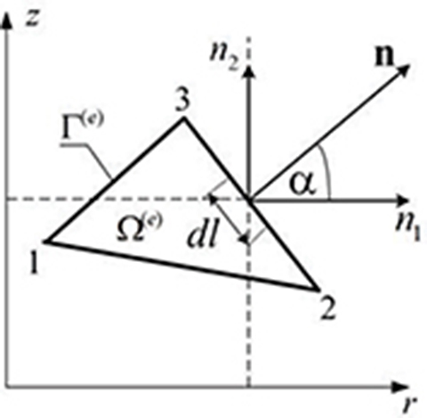
Fig. 4.2. Triangular element in axisymmetric coordinates.

$\begin{matrix} [A] = [\begin{matrix} A_{1}^{(e)} \\ A_{2}^{(e)} \\ A_{3}^{(e)} \end{matrix}] & [M] = [\begin{matrix} 1 r_{1} & z_{1} \\ 1 r_{2} & z_{2} \\ 1 r_{3} & z_{3} \end{matrix}] & [β] = [\begin{matrix} β_{1} \\ β_{2} \\ β_{3} \end{matrix}] \end{matrix} (4.61)$

After solving eqn (4.60), the values of the interpolation constants in eqn (4.59) can be determined, i.e.,

$[\begin{matrix} β_{1} \\ β_{2} \\ β_{3} \end{matrix}] = {[M]}^{- 1} [\begin{matrix} A_{1} \\ A_{2} \\ A_{3} \end{matrix}] = \frac{1}{2 S_{c}} [\begin{matrix} m_{11} & m_{21} & m_{31} \\ m_{12} & m_{22} & m_{32} \\ m_{13} & m_{23} & m_{33} \end{matrix}] [\begin{matrix} A_{1} \\ A_{2} \\ A_{3} \end{matrix}] (4.62)$

where

$\begin{matrix} 2 S_{c} = r_{1} (z_{2} - z_{3}) + r_{2} (z_{3} - z_{1}) + r_{3} (z_{1} - z_{2}) \\ {\begin{array}{l} m_{11} = r_{2} z_{3} - z_{2} r_{3} \\ m_{12} = z_{2} - z_{3} \\ m_{13} = r_{3} - r_{2} \end{array} \\ {\begin{array}{l} m_{21} = r_{3} z_{1} - z_{3} r_{1} \\ m_{22} = z_{3} - z_{1} \\ m_{23} = r_{1} - r_{3} \end{array} \\ {\begin{array}{l} m_{31} = r_{1} z_{2} - z_{1} r_{2} \\ m_{32} = z_{1} - z_{2} \\ m_{33} = r_{2} - r_{1} \end{array} \end{matrix}$

Thus, the value of the potential A in each element e can be expressed as

$A^{(e)} (r, z) = \frac{1}{2 S_{c}} [\sum_{j = 1}^{3} (A_{j}^{(e)} (m_{j 1} + m_{j 2} r + m_{j 3} z))] = \sum_{j = 1}^{3} A_{j}^{(e)} N_{j}^{(e)} (4.63)$

where

$N_{j} = \frac{1}{2 S_{c}} (m_{j 1} + m_{j 2} r + m_{j 3} z) (4.64)$

4.2.3 Commercial FEM Packages

Nowadays, many commercial packages are available for the FEM simulation of electromagnetic fields, e.g., MagNet from Infolytica Co., Montreal, Canada, Maxwell from Ansoft Co., Pittsburgh, PA, USA; Flux from Magsoft Co., Troy, NY, USA; JMAG from JMAG Group, Tokyo, Japan; and Opera from Vector Fields Ltd., Oxford, UK [13, 33, 193, 229]. All these packages have 2D and 3D solvers for electrostatic, magnetostatic and eddy-current problems. They are mostly based on PDEs. Eqns (4.9) or (4.6) can also be solved with the 2D codes, and this will be shown in Chapter 5 of this book.

Although, each computer package uses its own methodology, fundamental expressions arise from the theory of the electromagnetic field [25, 41, 226]. For example, the electromagnetic force has been obtained from Maxwell’s stress tensor, which can be written in the following general form:

$d F = (\frac{1}{2} (H(B \cdot n) + B(H \cdot n) - (H \cdot B)n)) \cdot d Γ (4.65)$

Each approach has its own merits and, in some cases, one cannot be conveniently substituted by the other.

4.3 Time-Stepping FEM Analysis

Time stepping FEM is a combination of the FEM and state space methods. It is used in the analysis and synthesis of electrical machines to increase the accuracy of simulation of dynamic characteristics.

The 2D problem in PM electrical machines can be described by the following equation [101, 242]:

$\frac{\partial}{\partial x} (\frac{1}{μ} \frac{\partial A}{\partial x}) + \frac{\partial}{\partial z} (\frac{1}{μ} \frac{\partial A}{\partial z}) = σ \frac{d A}{d t} - J_{a} - J_{M} (4.66)$

where A is the y-component (perpendicular to the plane of laminations) of the magnetic vector potential, μ is the permeability, σ is the electric conductivity, J_a is the current density of the armature (primary) winding, and J_M is the equivalent current density of the PM magnetization vector — see also eqn (3.83).

Images

Fig. 4.3. Flowchart of time-stepping FEM analysis.

Eqn (4.66) can be solved using appropriate boundary and initial conditions, i.e.,

Neumann boundary condition

$\frac{1}{μ} \frac{\partial A}{\partial n} = A_{1} (t) on Γ_{1} (4.67)$
homogenous Dirichlet boundary condition

$A = 0 on Γ_{2} (4.68)$
homogenous Neumann boundary condition

$\frac{\partial A}{\partial n} = 0 on Γ_{3} (4.69)$
initial condition

$\begin{matrix} A_{t = 0} = A_{0} (x, z) & for (x, z) belonging to the whole region \end{matrix} (4.70)$

where Γ₁+Γ₂+Γ₃ = Γ is the whole boundary around the calculation area. Applying Green’s identity and using the Bubnov–Galerkin’s method, eqn (4.66) can be transformed to

$\int_{S} \nabla N_{j}^{T} \frac{1}{μ} \nabla A d S + \int_{S} σ N_{j} \frac{d A}{d t} d S - \int_{S} N_{j} J_{0} d S - \int_{S} N_{j} J_{M} d S = 0 (4.71)$

where j=1, 2, 3 for triangular elements. Eqn (4.71) can be written in matrix form

$\sum_{e = 1}^{N_{e}} {{[K]^{(e)} [A]}^{(e)} + [C]^{(e)} \frac{d}{d t} [A]^{(e)} - [Q_{I}]^{(e)} [I]^{(e)} - {[Q_{M}]}^{(e)}} = [0] (4.72)$

where N_e is the total number of elements, [A] is the magnetic vector potential matrix, and [I] is the electric current matrix. The matrices [K] (m), [C] (S/m), and [Q_I] (dimensionless) in expression (4.72) include coefficients of the system of algebraic equations. The vectors [I] (A) and [Q_M] (A) are related to currents and PMs, respectively. The matrix [C] is the conductivity matrix representing the region with the reaction rail. The product [C]^(e) and $\frac{d}{d t} {[A]}^{(e)}$ is equal to the vector of eddy currents.

The matrix form of Kirchhoff’s voltage equation for the electric system is

${[V]}^{(e)} = (e) = [R]^{(e)} [I]^{(e)} + [L]^{(e)} \frac{d}{d t} [I]^{(e)} + [G]^{(e)} \frac{d}{d t} [A]^{(e)} (4.73)$

where [R], [L], and [G] are resistance, inductance, and conductance matrices, respectively. The conductance matrix [G] relates to the region with the armature winding. The product [G]^(e) and $\frac{d}{d t} {[A]}^{(e)}$ is equal to the voltage (EMF) induced in the armature winding. By applying Euler’s backward time difference method and assuming that the derivatives of [I] and [A] are

$\frac{d}{d t} [I] \approx \frac{[I]^{(t + Δ t)} - [I]^{(t)}}{Δ t} (4.74)$

$\frac{d}{d t} [A] \approx \frac{[A]^{(t + Δ t)} - [A]^{(t)}}{Δ t} (4.75)$

the whole electromechanical system matrix can be expressed as [101]

$\begin{matrix} [\begin{matrix} \begin{matrix} [K] + \frac{1}{Δ t} [C] \\ - [G] \end{matrix} & \begin{matrix} - [Q_{I}] \\ - [R] Δ t - [L] \end{matrix} \end{matrix}] [\begin{matrix} {[A]}^{(t + Δ t)} \\ {[I]}^{(t + Δ t)} \end{matrix}] \\ = [\begin{matrix} \frac{1}{Δ t} [C] [0] \\ - [G] - [L] \end{matrix}] [\begin{matrix} {[A]}^{(t)} \\ {[I]}^{(t)} \end{matrix}] + [\begin{matrix} {[Q_{M}]}^{(t + Δ t)} \\ - Δ t {[V]}^{(t + Δ t)} \end{matrix}] \end{matrix} (4.76)$

Compare also [50, 51]. The mechanical balance equation of the system is

$F_{d} - F = m \frac{d v}{d t} + D_{v} v (4.77)$

where D_v is the mechanical damping constant, v = dx/dt is the linear velocity, F_d is the electromagnetic force, and F is the external force. The electromagnetic force F_d can be calculated using e.g., Maxwell’s stress tensor. As the part of the mesh is moving with the displacement of the reaction rail, the moving mesh technique is used to model the movement of the reaction rail [242]. The flowchart of time-stepping FEM analysis is given in Fig. 4.3.

4.4 FEM Analysis of Three-Phase PM LSM

With the growing demand on LSMs, an accurate approach to their design is required. Nowadays, the FEM method is regarded as the most accurate computational tool and necessary, among others, for the calculation of inductances, forces, and operating characteristics. In this section, FEM calculations supported by analytical calculations for PM LSMs are discussed.

4.4.1 Geometry

The presented modular PM LSM can be built both in flat and tubular forms (Figs. 4.4 to 4.7). The flat topology is characterized by the rectangular form of the armature and reaction rail slices. The concentration of magnetic energy is in the air gap between the flat reaction rail (excitation system) with PMs of w_M thickness and the armature of l_M length (Fig. 4.5).

For the flat construction, the dimension l_M perpendicular to the plane of the longitudinal section (Fig. 4.5) is very important because the output power depends on that dimension. The armature and reaction rail are assumed to be of the same width l_M. For comparative analysis of the flat and tubular topologies, their electromagnetic parameters have been calculated.

4.4.2 Specifications of Investigated Prototypes of PM LSMs

Dimensions of investigated prototypes of PM LSMs (Figs. 4.5 and 4.7) are given in Table 4.1. Magnetization curves, i.e., B-H curve and relative magnetic permeability curve μ_r verus H of mild steel used for the investigated LSMs are plotted in Fig. 4.8. The electric conductivity of mild steel at 20°C is σ = 4.5 × 10⁶ S/m.

Images

Fig. 4.4. (see color insert.) Outline of 3-phase flat LSM. 1 — armature coil, 2 — ferromagnetic core, 3 — tooth of the armature segment, 4 — PM, 5 — flat ferromagnetic bar.

Images

Fig. 4.5. Dimensions of 3-phase flat LSM. 1 — armature coil, 2 — ferromagnetic core, 3 — tooth of the armature segment, 4 — PM, 5 — flat ferromagnetic bar.

Owing to the modular construction shown in Figs 4.4 to 4.7, it is possible to design a series of LSMs with different number of phases m₁. The formula for the appropriate distance between segments for a 3-phase motor is [220, 230]

$\begin{matrix} If, w_{s s} \leq \frac{4 τ}{3}, then d_{s} = k \cdot \frac{τ}{3} - w_{s s} + τ, k = 1, 2 \dots \\ else d_{s} = \frac{τ}{3} - w_{s s} + k \cdot τ, k = 1, 2 \dots \end{matrix} (4.78)$

where k is the smallest integer number for which d_s > 0. For the main dimensions of three-phase LSMs presented in Table 4.1 and magnetization curves shown in Fig. 4.8, the distance between segments is d_s = 2 mm (Figs. 4.5 and 4.7).

Images

Fig. 4.6. (see color insert.) Cutaway view of 3-phase tubular LSM. 1 armature segment, 2 — armature coil, 3 — nonferromagnetic ring, 4 — armature cover, 5 — PM, 6 — ferromagnetic ring, 7 — nonferromagnetic tube, 8 — linear slide bearing.

Images

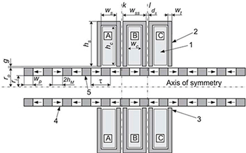
Fig. 4.7. Longitudinal section of 3-phase tubular PM LSM. 1 — armature coil, 2 — ferromagnetic core, 3 — tooth of the armature segment, 4 — PM, 5 — ferromagnetic ring.

Table 4.1. Main dimensions of prototypes of PM LSMs shown in Figs. 4.5 and 4.7

Images

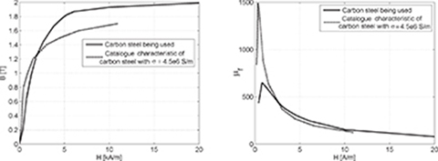
Fig. 4.8. Magnetization curves of mild steel used for the investigated prototypes of PM LSMs: (a) B-H curves; (b) relative magnetic permeability μ_r verus H curves.

Images

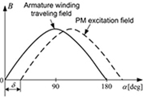
Fig. 4.9. Load angle δ defined as angular displacement between PM magnetic flux density and armature magnetic flux density waveforms (see also Fig. 3.1).

Images

Fig. 4.10. Portion of the discretization mesh for 3-phase PM LSMs: (a) flat motor, (b) tubular motor.

The load angle δ is defined as the angular displacement between the zero crossings of the excitation field waveform and traveling field waveform generated by the armature winding, as shown in Fig. 4.9. The electromagnetic force (thrust) is produced only when the load angle δ ≠ 0. The maximum force is for the load angle δ = 90° (see Fig. 3.2).

4.4.3 Approach to Computation

In calculating the magnetic flux density and other integral parameters, displacement currents and eddy currents have been neglected. The partial saturation of the reaction rail has been included, especially for the maximum allowable current. The electromagnetic field is governed by the PDE of elliptic type (4.51).

The computation process involves the following steps: modeling the geometry, setting boundary conditions and properties of each region, generating the finite element mesh, solving eqn (4.51), and calculating the field integral parameters. After drawing the outline of the armature and reaction rail (Figs. 4.5 and 4.7), the physical properties of materials have been introduced.

The Dirichlet conditions A_φ = 0 at the boundaries of the geometric model have been predefined. The triangular finite element mesh has been generated. For solution of the PDE, the nonlinear solver has been employed [41, 212]. For each position of the reaction rail, to minimize errors (in differentiation or integration of the magnetic potential), a nonuniform grid has been created, so that its refinement was extremely near the edges of the reaction rail.

4.4.4 Discretization of LSM Area in 2D

The field problems for the LSM have been solved in 2D regions by solving the PDE equation (4.51) with the Dirichlet boundary conditions. An exemplary mesh of finite elements inside the motor is shown in Fig. 4.10. Two non-ferromagnetic distance layers with their thickness of 2 mm between armature segments have been inserted (4.6). In the vicinity of the outer surface of the armature core crude nonferromagnetic rings (4-mm thickness) have been placed (Figs. 4.6 and 4.10). The cuts in outer rings are visible in Fig. 4.10, as well as in Figs 4.11 and 4.12.

As previously mentioned, a fine mesh is required in FEM modeling. This mesh should be dense enough to minimize the calculation error. On the other hand, more dense discretization causes longer time of computations (solution to eqn (4.44)). Thus, it is important to optimize the finite element mesh. Modern mesh generators can find a compromise between accuracy and computation time.

Images

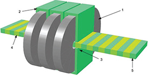
Fig. 4.4. Outline of 3-phase flat LSM. 1 — armature coil, 2 — ferromagnetic core, 3 — tooth of the armature segment, 4 — PM, 5 — flat ferromagnetic bar.

Images

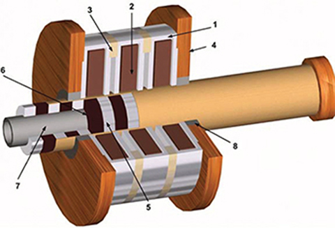
Fig. 4.6. Cutaway view of 3-phase tubular LSM. 1 armature segment, 2—armature coil, 3 — nonferromagnetic ring, 4 — armature cover, 5 — PM, 6 — ferromagnetic ring, 7 — non-ferromagnetic tube, 8 — linear slide bearing.

Images

Fig. 4.11. Magnetic field distribution in longitudinal sections of 3-phase PM LSMs at no-load (δ = 0): (a) flat motor, (b) tubular motor.

Images

Fig. 4.22. Magnetic flux density maps in the case of excitation by the imaginary components of armature currents: (a) flat motor, (b) tubular motor.

Images

Fig. 8.4. Transrapid 07 Europa (Emsland Transrapid Test Facility). Photo courtesy of Thyssen Transrapid System, GmbH, München, Germany.

Images

Fig. 8.9. Transrapid 08. Photo courtesy of Thyssen Transrapid System, GmbH, München, Germany.

Images

Fig. 8.11. Transrapid in Shanghai, China.

Images

Fig. 8.13. Yamanashi Maglev Test Line: Ogatayama Bridge over the Chuo Expressway. Courtesy of Central Japan Railway Company and Railway Technical Research Institute, Tokyo, Japan.

Images

Fig. 8.19. Double-cusp-shaped head car (facing Koufu) of the MLX01 Maglev Train at Expo 2005, Aichi Prefecture, Japan. Courtesy of Central Japan Railway Company and Railway Technical Research Institute, Tokyo, Japan.

Images

Fig. 8.25. Prototype of urban maglev vehicle built by General Atomics, San Diego, CA, USA. Photo taken by the first author.

Images

Fig. 8.28. Principle of operation of General Atomics’ maglev vehicle. 1 — upper Halbach array levitation magnets, 2 — lower Halbach array levitation magnets, 3 — Litz wire guide-way, 4 — LSM armature winding, 5 — propulsion magnets. Photo taken by the first author.

Images

Fig. 8.29. Cross section through the station of Swissmetro. Courtesy of Swissmetro, Geneva, Switzerland.

Images

Fig. 4.11. (see color insert.) Magnetic field distribution in longitudinal sections of 3-phase PM LSMs at no-load (δ = 0): (a) flat motor, (b) tubular motor.

Images

Fig. 4.12. Magnetic field distribution in longitudinal sections of 3-phase PM LSMs at full load (δ = 90°): (a) flat motor, (b) tubular motor.

Images

Fig. 4.13. Maximum thrust versus reaction rail position for tubular and flat three-phase PM LSMs.

4.4.5 2D Electromagnetic Field Analysis

The calculated magnetic flux lines in 3-phase PM LSMs are presented in Figs 4.11 to 4.12. Rare-earth sintered NdFeB grade 35 PMs with remanent magnetic flux density B_r = 1.25 T and coercivity H_c = −950 kA/m at 20°C have been employed. The relative recoil magnetic permeability is μ_rrec = 1.048. Both flat and tubular motors have been considered. The 2D field distribution has been obtained for two load angles: δ = 0 as shown in Fig. 4.11 and δ = 90° as shown in Fig. 4.12. The maximum armature current is I_a = 8 A (Table 4.2). Various shades of grey color denote magnetic flux density values. For the field distribution, the position of three-phase balanced currents is shown in the right top corner. The value of the current at the calculated time instant can be obtained as a projection of the current phasor onto the vertical axis in the complex plane. Under the same supply and load, the magnetic flux density distributions are similar for both flat and tubular motors. However, for the flat motor (Figs. 4.11a and 4.12a), the magnetic flux density distribution in the stator segments is more homogenous as compared with the tubular motor (Figs. 4.11 and 4.12b).

In the tubular LSM, the highest magnetic flux density, as expected, is observed in the region of armature teeth close to the air gap. The lowest magnetic flux density is seen close to the outer surface of the armature core. This is because the cross section of the magnetic flux increases with the radius. The magnetic flux that links the coil turns depends on the input voltage, which causes an increase in the armature current. The magnetic flux is a nonlinear function of the armature current. Consequently, the magnetic saturation depends on the armature current I_a. For the armature current I_a = 8 A, some portions of the magnetic circuit become highly saturated (Figs. 4.11 and 4.12).

Comparative analysis of the magnetic field distribution in tubular and flat LSMs allows for formulating recommendations of how to size the motor. To obtain similar parameters of a flat LSM to those of a tubular LSM, the width l_M of the flat motor can be assumed to be equal to the circumference of the air gap of the tubular motor. The FEM analysis shows that the magnetic saturation effect is less pronounced in a flat motor than in a tubular motor.

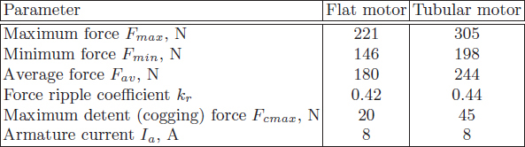
Table 4.2. Electromagnetic thrust under rated (nominal) current for the analyzed flat and tubular three-phase PM LSMs

Images

4.4.6 Calculation of Integral Parameters

The thrust F is the most important parameter of linear motors. In Figs. 4.13 and 4.14, the thrust is plotted against the position of the reaction rail under rated (nominal) armature current.

Forces F_max, F_min, and F_av denote maximum, minimum, and average value of the trust at nominal load angle (Section 4.4) under nominal armature current I_a. The force F_cmax is the maximum value of the detent force i.e., the force due to interaction of PM and armature ferromagnetic teeth (salient poles) at zero current state. The force ripple coefficient k_r has been calculated using the formula

$k_{r} = \frac{F_{m a x} - F_{m i n}}{F_{a v}} (4.79)$

Both the useful electromagnetic thrust and force ripple coefficient k_r are lower in the case of the flat motor.

Although, the results of the 3D analysis are similar to those obtained from the 2D analysis, in both cases of flat and tubular construction, the forces obtained from the 3D simulation are lower. In PM motors, the detent (cogging) thrust affects the useful thrust. The peaks of the thrust are slightly greater in the case of the tubular motor (Figs 4.15 and 4.16). The results of the 2D and 3D FEM analysis clearly show this difference. In fact, the paths of the magnetic flux in a flat motor are closed through the front and back parts of the motor. To minimize the computation time, the 3D analysis has been performed with 1-mm step, and the 2D analysis with 0.25-mm step. Thus, the waveforms obtained from the 2D FEM are smoother (Fig. 4.16).

Images

Fig. 4.14. Comparison of thrust obtained from 2D and 3D FEM computations: (a) tubular motor, (b) flat motor.

Images

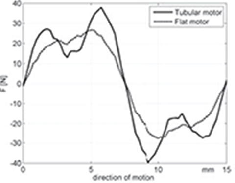
Fig. 4.15. Detent force for the tubular and flat PM LSMs.

Images

Fig. 4.16. Comparison of detent forces obtained from 2D and 3D FEM computations: (a) tubular motor, (b) flat motor.

The electromagnetic thrust distribution under the net load angle δ = 0 is shown in Figs 4.17 and 4.18. The higher thrust is observed in the case of three-phase tubular motor. The shapes of thrust waveforms of the flat and tubular motors differ significantly (Fig. 4.17). The differences between the 2D and 3D computations are due to air gap discretization and, in the case of the flat motor, due to the construction. It should be emphasized that the flat construction can be analyzed as a 2D problem without significant loss of accuracy.

Images

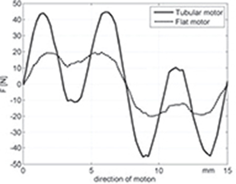
Fig. 4.17. Thrust at δ = 0 versus position of reaction rail.

Images

Fig. 4.18. Force at δ = 0 obtained from 3D FEM computations: (a) tubular motor, (b) flat motor.

Examples

Example 4.1

Two three-phase PM LSMs have been studied. The first one is a tubular linear motor (Fig. 4.6) and the second one is a flat motor (Fig. 4.5). The reaction rail (moving part) has been assembled with ring-shaped NdFEB magnets (2h_M = 8 mm) and mild steel rings (w_p = 7 mm). The dimensions of the tubular LSM are shown in Figs 4.7 and 4.19. The flat LSM has the same cross-sectional dimensions, while its width l_M = 48.7 mm. The three coils, each with N = 280 turns, are excited with 3-phase sinusoidal armature current the amplitude of which is I_m = 8 A.

The objective is to compare the magnetic field distributions excited by the imaginary components of the current system depicted in Fig. 4.19, when the reaction rail is in an aligned position. Also, the modulus of the flux density in the middle of the air gap of both machines should be compared (along section AA’ shown in Fig. 4.19). The comparison should be performed for the reaction rail in the aligned position (Fig. 4.19) and for the armature alone, without the reaction rail. The aligned position of the reaction rail is the initial position (z = 0) as well. The positive z coordinate is assumed to be in the right direction. Additionally, the inductance of the coil C should be found. For the current system depicted as in Fig. 4.19, the load angle takes its maximum value δ = 90°.

Solution

This problem has been solved using the 2D FEM freeware program written by D. Meeker [144].

First, the final element mesh is created. The portion of the motor geometry being analyzed is shown in Fig. 4.20. An appropriate discretization is the second important step in electromagnetic field modeling. The triangular mesh has been implemented (Fig. 4.21). To obtain high accuracy of calculation of the electromagnetic force, the air gap should be discretized very precisely (the largest segment of elements should not exceed 0.3 mm in length). The force acting on the reaction rail is calculated using Maxwell’s stress tensor. In this case, the reaction rail should be surrounded with a contour line that is placed 0.5 mm away from the reaction rail [144]. At the outside boundaries (not visible in the figures), the Dirichlet boundary condition A = 0 has been applied. The B-H curve of the mild steel is shown in Fig. 4.8a (solid line). The sintered NdFeB PMs have the remanent magnetic flux density B_r = 1.25 T and coercivity H_c = 950 kA/m at room temperature 20°. The phase currents are:

$\begin{matrix} i_{a A} (z) = I_{m} sin(\frac{z}{τ} 180^{0} + 150^{0} + δ) \\ i_{a B} (z) = I_{m} sin(\frac{z}{τ} 180^{0} - 90^{0} + δ) \\ i_{a C} (z) = I_{m} sin(\frac{z}{τ} 180^{0} + 30^{0} + δ) \end{matrix} (4.80)$

Images

Fig. 4.19. Dimensions of the analyzed three-phase tubular LSM and current phasor diagram. The reaction rail is in aligned position.

Images

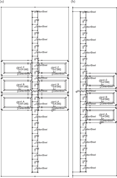
Fig. 4.20. Outline of the geometry of motors for FEM modeling: (a) flat motor, (b) tubular motor.

Images

Fig. 4.21. Portions of the mesh for: (a) flat construction, (b) tubular motor.

For the position z = 0 and the maximum load angle δ = 90° the values of the imaginary components of the armature currents are I_aA = −6.93 A, I_aB = 0, I_aC = 6.93 A (Fig. 4.19, left top corner).

Fig. 4.22 shows the magnetic flux density distributions. The flux lines are similar both for tubular and flat motors. The highest magnetic saturation is observed in the third segment (I_aA = −6.93 A). For the load angle δ = 90°, in the aligned position of the reaction rail (Fig. 4.19), only two segments (phase A and C) generate the thrust. The middle segment (phase B) does not contribute to the resultant thrust.

Images

Fig. 4.22. (see color insert.) Magnetic flux density maps in the case of excitation by the imaginary components of armature currents: (a) flat motor, (b) tubular motor.

The flux density waveforms are similar both in flat and tubular motors. It is clearly visible from Fig. 4.22 that the main flux is generated by PM filed excitation system. The armature current (LSM without reaction rail) contributes only minimally to the total flux density distribution, which does not exceed B = 0.2 T.

Peak values of the air gap magnetic flux density in the AA‘ section (Fig. 4.19) are plotted in Fig. 4.23. For the tubular motor, the maximum magnetic flux density is inside the first tooth region of the phase A (B = 1.9 T).

Images

Fig. 4.23. Magnetic flux density distribution along the z-coordinate: (a) in the air gap, (b) near the armature core with reaction rail being removed.

The winding inductance of the coil C is calculated using eqn (4.17) or (4.18) given in Section 4.1. In the case of an assembled motor (with reaction rail), the static inductance (4.17) is L_s = 7 mH for the flat motor and L_s = 12.7 mH for the tubular motor. In the case of a disassembled motor without the reaction rail, L_s = 10.5 mH for the flat motor and L_s = 16.7 mH for the tubular motor. The inductance of the assembled motor is greater than that of the disassembled motor because of greater linkage flux. The presence of magnetic flux excited by PMs reduces the linkage flux. The lower values of the inductance for the flat motor are due to simplification of the 3D geometry in the 2D analysis. The end turns (overhangs) of the armature coils have been neglected in the 2D analysis.

The electromagnetic thrust (force) is the most important parameter of a linear motor. To calculate the thrust using Maxwell’s stress tensor, the contour of the integration line should be as close as possible to the surface of the reaction rail. In this case, the integration line was at the distance of 0.5 mm from the surface of the reaction rail. The computed thrust is F = 195 N for the flat LSM and F = 268 N for the tubular LSM.

Images

Fig. 4.24. Dimensions of the analyzed three-phase tubular PM LSM and current phasor diagram. The system of the armature currents for z = 0 and δ = 90° is shown in the left top corner.

Example 4.2

Find the magnetic field distribution and its integral parameters for a three-phase tubular LSM with dimensions given in Fig. 4.24 (aligned initial position of the reaction rail). Use the FEM approach. The parameters of the materials including B-H curves for the armature core and reaction rail are the same as in Example 4.1 (Fig. 4.8a, solid line). The mesh and boundary conditions are assumed to be similar to those in Example 4.1. The wire diameter of the armature coils is 1.5 mm and number of turns N = 190. The coils are fed with sinusoidal current the peak value of which is I_m = 9 A. The load angle has been set as δ = 90°. The coil inductances and thrust should be calculated versus the position of the reaction rail in the interval 0 ≤ z ≤ 21 mm.

Solution

To hold the load angle δ = 90° for the whole range of reaction rail positions, the phase currents must be functions of position of the reaction rail. Three-phase currents are expressed as

$\begin{matrix} i_{a A} (z) = I_{m} sin(\frac{z}{τ} 180^{0} - 30^{0} + δ) \\ i_{a B} (z) = I_{m} sin(\frac{z}{τ} 180^{0} + 90^{0} + δ) \\ i_{a C} (z) = I_{m} sin(\frac{z}{τ} 180^{0} + 210^{0} + δ) \end{matrix} (4.81)$

Images

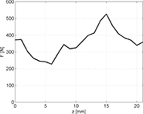
Fig. 4.25. Maximum thrust at δ = 90° versus the position of the reaction rail.

The FEM package created by D. Meeker has been used [144]. Computation results are presented in Figs 4.25, 4.26, and 4.27. The thrust (Fig. 4.25) changes from 220 N up to 520 N, depending on the position of the reaction rail. Fig. 4.25 also shows that the LSM produces high thrust ripple. The objective function in the optimization procedure should be minimization of the thrust ripple to obtain smoother distribution of the thrust versus the position of the reaction rail.

The static inductance L_s fluctuates with the position of the reaction rail (Fig. 4.26). This is due to interaction of the PM field and armature winding currents. In some positions of the reaction rail, the flux lines have opposite directions, but they coincide one with the other. The main field excitation originates from the PM system so that it always exists in the air gap. Thus, at some positions of the reaction rail, a coil can be coupled with the magnetic flux, although there is no armature current. In these cases, the static inductance tends to infinity. Sometimes, the PM flux and armature reaction flux neutralize each other, which results in the net value of the static inductance L_s.

The magnetic flux distribution is presented in Fig. 4.27 for two positions of the reaction rail, i.e., z = 6 mm and at z = 15 mm. At z = 6 mm, the thrust achieves its minimum value, and z = 15 mm, the thrust achieves its maximum value. In both cases, the highest concentration of the magnetic flux lines is in the armature tooth area, in particular at the corners.

Example 4.3

Calculate the main dimensions of a three-phase tubular PM LSM that produces the maximum thrust F_max = 1000 N. The outline of the motor is given in Fig. 4.6. Dimensions are marked in Fig. 4.7.

The nominal peak current density in the armature winding is assumed as J_a = 10 A/mm². The magnets are made from sintered NdFeB with remanent magnetic flux density B_r = 1.25 T and coercivity H_c = 950 kA/m at room temperature 20°C. All ferromagnetic parts are made from typical mild steel with the B-H curve plotted in Fig. 4.8a, solid line. The desired maximum value of the magnetic flux density in the air gap is around B_g = 1.5 T. The wire diameter of the armature winding is d_w = 2 mm.

Images

Fig. 4.26. Variation of static inductance of the coils with the position of reaction rail for δ = 90°: (a) coil A, (b) coil B, (c) coil C.

Solution

The magnetic flux density in the air gap is set at B_g = 1.5 T. The thrust developed by one segment is estimated on the assumption that the leakage and fringing fluxes are neglected. If the magnetic flux crossing the A-surface of the air gap is known, the electromagnetic force (thrust) can be calculated on the basis of eqn (1.15)¹, i.e.,

Images

Fig. 4.27. Magnetic field distribution at load angle δ = 90° for: (a) z = 6 mm (minimum thrust); (b) z = 15 mm maximum thrust).

$F = \frac{B_{g}^{2} A}{2 μ_{0}}$

where B_g is the magnetic flux density in the air gap, A = 2(2πrw_t) is the surface area of air gaps between the armature teeth and the reaction rail (area of two poles North and South), and r is the inner radius of the armature core. Thus, the surface

$A = \frac{2 F μ_{0}}{B_{g}^{2}} = \frac{2 \times 1000 \times 0.4 π \times 10^{- 6}}{{1.5}^{2}} = 1.117 \times 10^{- 3} m^{2}$

Either the width of teeth or their radii are to be known. Putting the inner armature core radius r = 0.5D_1in = 18 mm and the outer radius of the reaction rail r_o = 17 mm, the width of each tooth is

$w_{t} = \frac{1}{2} \frac{A}{2 π r} = \frac{1.11.7 \times 10^{- 3}}{4 \times 314 \times 0.018} = 4.941 mm$

The width of the tooth can be rounded to w_t = 5 mm. The dimensions of the magnets and ferromagnetic rings should match each other, e.g., the width of the magnet and ferromagnetic ring is twice the width of the armature tooth, i.e.,

$2 h_{M} = w_{p} = 2 \cdot w_{t} = 10 mm$

The inner radius of a PM and ferromagnetic ring should be as small as possible, e.g., r_i = 4 mm. Typically, the inner radius should be less than 1/4 of the outer radius, i.e., r_i < 0.25r_o. The inner radius r_i is the same as the outer radius of the nonferromagnetic rod, which keeps all parts of the reaction rail together.

The MMF of the PM depends on its coercivity H_c and height h_M per pole, i.e.,

$F_{M} = 2 h_{M} H_{C} = 0.01 \times 950000 = 9500 A$

Because of the armature reaction, which can weaken the PM excitation field, the armature MMF should be less than half of the magnet MMF. Since the maximum current density and wire diameter (d_w = 2 mm) are known, the maximum armature current can be calculated as

$I_{a m a x} = J_{a} \frac{π d_{w}^{2}}{4} = 10 \times \frac{π \times {2.0}^{2}}{4} = 31.4 A$

The number of turns per one coil can be calculated on the basis of the magnet MMF, i.e.,

$N = \frac{F_{M} / 2}{I_{a m a x}} = \frac{4750}{31.4} = 151.27$

The number of turns per coil is rounded to N = 151. To build a tubular PM LSM using separate segments, as shown in Fig. 4.6, the width of the segment “window” w_s has to satisfy the condition

$2 h_{M} \leq w_{s} \leq τ - w_{t}$

Thus 10 mm ≤ w_s ≤ 15 mm. Assuming w_s = 13 mm, the width of the coil can be w_c = 11 mm. The coil height h_c can be found on the basis of the coil width w_c and number of turns, i.e.,

$h_{c} = d_{w}^{2} \frac{N}{w_{c}} = {2.0}^{2} \frac{151}{11} \approx 55 mm$

Images

Fig. 4.28. Main dimensions of the designed tubular PM LSM.

The distance d_s between segments is calculated using condition (4.78):

$d_{s} = \frac{τ}{n_{ph}} - w_{s s} + τ = \frac{20}{3} - 23 + 20 = 3.67 mm$

All calculated dimensions are shown in Fig. 4.28. The 2D FEM computations give the average force value F_av = 805 N. The force versus the position of the reaction rail has been calculated in the same way as in Example 4.1. The maximum force reaches F_max = 930 N. Thus, the value obtained from the FEM computations is 7% lower than the target maximum thrust F_max = 1000 N. The designed tubular PM LSM is characterized by high detent force (Fig. 4.29). Optimization of the LSM construction is needed to minimize the detent force. Possible independent variables in the optimization procedure include the width of armature tooth w_t, distance between stator segments d_s, height of the PM 2h_M in the axial direction, width of the ferromagnetic rings w_p, and outer diameter of the reaction rail 2R_o. Additionally, the shape of the armature tooth can be changed since the concentration of the magnetic flux lines is observed in the tips of teeth (Fig. 4.30). It is also possible to design the PM LSM with two or more armature segments per one phase. In this case, the outside LSM diameter will decrease, and the axial length of the armature system will increase.

Example 4.4

Calculate the main dimensions of a three-phase tubular PMS LSM, which produces the maximum thrust F_max = 1000 N. Verify the thrust with the FEM method. Assume the nominal armature current density J_a = 10 A/mm², wire diameter d_w = 2 mm, and the pole pitch τ = 50 mm. Calculate the dimensions of PMs under assumption that the mechanical energy is equal to the energy stored in the PMs. In order to produce the expected thrust, at least 7 PMs and 3 segments of the armature system are needed. The magnets are made of sintered NdFeB with remanent magnetic flux density B_r = 1.25 T and coercivity H_c = 950 kA/m at 20°C, and the all ferromagnetic parts are made from typical mild steel (Fig. 4.8a, solid line). The expected magnetic energy density of the magnet is w = 400 kJ/m³.

Images

Fig. 4.29. Thrust versus position of the reaction rail at δ = 90°.

Solution

The energy needed to move the reaction rail with the electromagnetic force F = 1000 N along the distance τ = 50 mm is

$W = F τ = 1000 \times 0.05 = 50 J$

The volume V of all seven magnets is calculated from the energy W = 50 J and assumed energy density w = 400 kJ/m³, i.e.,

$V = \frac{W}{w} = \frac{50}{400000} = 1.25 \times 10^{- 4} m^{3} = 1.25 \times 10^{5} {mm}^{3}$

The volume of a single magnet V_M of the field excitation system consisting of seven PMs is V_M = V/7 = 17860 mm³.

Now, the dimensions of the PMs must be estimated. Since the pole pitch is τ = 50 mm, and assuming the same dimensions of the magnets and ferromagnetic rings, the width of a single magnet is

$2 h_{M} = w_{p} = \frac{τ}{2} = 25 mm$

Images

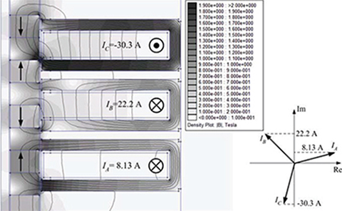
Fig. 4.30. Magnetic field distribution in the longitudinal section of the motor at z = 15 mm and δ = 90°.

The inner radius of PMs and ferromagnetic ring should be as small as possible, e.g., r_i = 4 mm. The outer diameter of the PM is

$r_{o} = \sqrt{\frac{V_{M}}{π (2 h_{M})} + r_{i}^{2}} = \sqrt{\frac{17860}{π \times 25} + 4^{2}} \approx 16 mm$

The width of the armature tooth should be a half of the width of the ferromagnetic ring, i.e.,

$w_{t} = \frac{w_{p}}{2} = \frac{25}{2} = 12.5 mm$

The MMF of the PM per two poles is

$F_{M} = 2 h_{M} H_{C} = 0.025 \times 950000 = 23750 A$

The maximum current density and wire diameter are known (d_w = 2 mm), so that the maximum value of the current is

$I_{a m a x} = J_{a} \frac{π d_{w}^{2}}{4} = 10 \frac{π \times {2.0}^{2}}{4} = 31.4 A$

The number of turns per coil is

$N = \frac{F_{M} / 2}{I_{a m a x}} = \frac{23750 / 2}{31.4} \approx 378$

To design a tubular PM LSM with separate segments (Fig. 4.7), the width of the “window” w_s has to satisfy the condition

$2 h_{M} \leq w_{s} \leq τ - w_{t}$

so that 25 ≤ w_s ≤ 37.5 mm. The width w_s of the “window” of each segment can be calculated as the arithmetic mean value of the maximum and minimum width, i.e., w_s = 0.5(25.0 + 37.5) = 31.25 ≈ 32.0 mm. If the insulation of the coil is 1 mm thick, the width of the coil is w_c = 30 mm. Since the distance between wires along the symmetry axis z and in the radial direction is the same, the number of turns per coil can be found as

$N = \frac{w_{c}}{d_{w}} \frac{h_{c}}{d_{w}}$

Thus, the height of the coil

$h_{c} = d_{w}^{2} \frac{N}{w_{c}} = {2.0}^{2} \times \frac{378}{30} \approx 50 mm$

The distance between segments is

$d_{s} = \frac{τ}{n_{ph}} - w_{s s} + τ = \frac{50}{3} - 57 + 50 = 9.67 mm$

Images

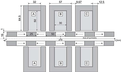
Fig. 4.31. Dimensions of the designed tubular PM LSM.

Images

Fig. 4.32. Magnetic flux density distribution in the longitudinal section of the motor (Fig. 4.31) for z = 38 mm and load angle δ = 90°.

Images

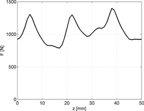
Fig. 4.33. Thrust versus position of reaction rail for δ = 90°.

The dimensions of the motor are shown in Fig. 4.31. For such estimated dimensions, the FEM package can be used to find the electromagnetic field distribution and electromagnetic forces. The magnetic flux distribution as obtained from the 2D FEM is shown in Fig. 4.32. The flux has been obtained under assumption of imaginary values of the three-phase current system shown in Fig. 4.33. Saturation of armature segments exists only in their inner areas, close to the air gap (smaller cross-section area for the magnetic flux).

The thrust versus the position of the reaction rail has been found from the integration of Maxwell stress tensor (Fig. 4.33). The average force F_av = 1043 N. The maximum value of the force is F_max = 1397 N. Thus, the value of the maximum force is 40% greater than the target value of the thrust F_max = 1000 N. The drawback of the construction shown in Fig. 4.31 is high detent force (force ripple). Minimization of the detent force can be done through the optimization process.

^¹This equation expresses the attraction force of an electromagnet. However, it can be used for simplified calculation of the thrust of a tubular PM LSM at zero armature current (I_a = 0 A) provided that the armature tooth and PM are in misaligned position.

..................Content has been hidden....................

You can't read the all page of ebook, please click here login for view all page.

Table of Contents for 4 FEM Analysis

Create new playlist

Sign In

Sign Up

Table of Contents for
4 FEM Analysis