
7
Sensors
7.1 Linear Optical Sensors
The encoder functioning as a feedback device is one of the basic components of motion control systems. There are four different sensor technologies used in linear servo applications, i.e., resistive, inductive, magnetic, and optical. The least complicated structure has a linear position transducer. Its principles of operation are based on the conversion of linear motion into rotation that is measured with the use of a precision potentiometer, tachometer, or digital encoder. However, the earliest linear encoders utilized in high-precision machines, e.g., in metal-cutting industry, were optical. Although other techniques are also now available, optical encoders are still predominant in industrial applications. In linear motor drives, where precision actuation and measurement are involved, most designers employ an incremental optical encoder as a well-accepted part of the electromechanical drive system. The typical optical encoder makes use of a graduated scale that is scanned by a movable optical readhead. The most important advantage of optical encoders is their easily achievable noncontact operation that eliminates friction and wear and permits reliable high-speed performance in workshop environments. Linear optical encoders are capable of achieving very high resolution, in some cases comparable to the laser interferometry technology. Their accuracy is a few orders of magnitude higher than that of similar resistive, magnetic, or inductive linear encoders. This is possible due to the superior precision of interpolation performed on much smaller-scale grating periods. The interpolation is a self-subdivision process of the signal representing the scale period.
7.1.1 Incremental Encoders
There are two basic methods of generating optical encoder signals. In the first method, the transmitted light is processed (Fig. 7.1a), while the second method employs reflected light (Fig. 7.1b).

Fig. 7.1. Typical scanning methods: (a) transmitted light method, (b) reflected light method. 1 — scale reflective tape, 2 — scale transparent glass, 3 — scanning reticle, 4 — condenser lens, 5 — light source (LED), 6 — photodetectors, 7 — reference mark.
The simplest configuration of an optical encoder is described here. The light emitted by an LED either travels through, or reflects off, the scale. It is then directed through an identical index grating and onto photo detectors that generate electrical currents. When the scanning units move, the scale modulates the light, producing sinusoidal outputs from the sensors. There are five windows in the scale reticle. Four of them are phase-shifted 90° apart. The readhead’s electronics combines the phase-shifted signals to produce two sinusoidal outputs. Twin signals s1 and s2, 90° out of phase, representing sine and cosine waveforms are generated. A fifth window on the scanning reticle has a random pattern graduation that creates a reference signal when aligned with identical pattern on the scale. The simplified optical incremental encoder consisting of light source, glass scale, scanning reticle, and two photodetectors shown in Fig. 7.2 illustrates the principles of forming s1 and s2 signals. The photo detector reads the maximum luminous intensity when transparent slots of the scale fully align with transparent slots of the scanning reticle. The light source and the photo detectors move along the glass scale grating. In consequence, the transparent slots of the scanning reticle change periodically their position relative to the stationary slots of the scale. Therefore, the light intensity detected by the photo sensors (photo elements) changes its value from maximum to zero according to a sinusoidal function (Fig. 7.2). Because the photo elements are displaced by the distance equal to one quarter of the scale grating period τp, when one photo element detects the maximum, the other one reads only half of the maximum. This displacement effectively shifts the two signals s1 and s2 by 90° in phase within the frequency domain. The 90° electrical separation or one quarter of the period between the two signals is referred to as the quadrature. Signals in the quadrature permit determination of the motion direction and speed at the same time allowing additional resolution through edge counting.
Linear motors employed in the x-y positioning stages and used in harsh factory or workshop environments require precise resolution with high reliability. The combination of a reflective, flexible scale tape placed along the track, and the readhead moving over the tape, offers many unique features.
The scale is made out of steel ribbon 5 to 10 mm wide and 0.2 mm thick, which has relatively low stiffness. Other materials, such as glass, mylar, or nonferrous metal tapes, can also be used. The scale is grated with alternating reflective strips (often made out of gold) and light-absorbing spaces. The grating period ranges from 100 to less than 20 μm, and after interpolation, resolution up to 0.1 μm is possible. The scale can be secured to the most commonly used materials (metals, composites, and ceramics) by means of a double-sided, elastic adhesive tape to accommodate the thermal expansion of the base. However, the mounting surface should be relatively smooth, clean, and parallel to the axis of motion with the scale ends rigidly fixed to the axis of the substrate. The location of stationary scale and moving readhead mounted on a positioning stage is shown in Fig. 7.3. The differential movement between the scale and the substrate should be close to zero, even in the presence of large temperature gradients. Usually, the scale tape is protected by varnish coating to facilitate easy cleaning. Scale tapes are generally supplied on a reel for ’cut–to–suit’ convenience. For comparison, glass scales reach maximum length of 3 m in a single piece. Usually, the incremental tapes are installed together with the reference marks. Limit switches are separately installed next to the scale itself. These home position and/or zero point indicators for the end of travel are also sensed by the scanning readhead. The signals are synchronized with the incremental channels to guarantee repeatability.

Fig. 7.2. Generation of photo detector signals: (a) photoelectric scanning setup; (b), (c), (d) examples of relative scale grating and scanning reticle positions; (e) corresponding signal variation. 1 — light source (LED), 2 — glass scale grating, 3 — scanning reticle, 4 — light rays, 5 — photodetectors.
The principle of the scanning process can be exemplified by the LIDA linear encoder, which was introduced to the market in 1977 by Heidenhain GmbH, Traunreut, Germany [84]. The operation of the LIDA encoder is explained in Fig. 7.1b. The redhead travels along the scale, while a light beam emitted by an LED source is directed onto the incremental scale grating through a condenser lens and scanning reticles. Then, it is reflected, and after passing back through the reticles, it is focused onto the photoelectric cells. Photo sensors detect changes in the light intensity caused by the interaction between the scale and reticle gratings. The four sinusoidal scanning signals, corresponding to the changes in the light intensity, are produced by the sensors. These waveforms with 90° phase shift enable formulation of symmetrical encoder zero output signals.

Fig. 7.3. Typical location of the linear encoder installed in the positioning stage driven by a linear motor. 1 — scale, 2 — readhead.
To improve the accuracy, especially in high-precision positioning applications within microelectronics industry, encoders frequently use interferential scanning principles. The diffracted (interferential) light method is required in the optical encoders with grating periods τp < 8 μm. These devices employ a reflection-type diffraction grating fixed to the carrier (Fig. 7.4). An infrared LED emits light onto angular scale facets where it is scattered back into the readhead through the transparent grating. The periodic pattern on the scale and the periodic indexing of the grating produce sinusoidal interference fringes at the photodetector plane. The fringes move across the detector plane as the readhead moves along the scale. The arrangement of interlaced groups of photodetectors positioned in repeating patterns generates electric signals related to the fringe movement. The readhead electronics processes these signals and generates two sinusoidal waveforms of equal amplitude with the phase shift of 90°. In RGH encoders manufactured by Renishaw plc, the signal is averaged from over 80 facets in the detector plane. Therefore, the loss of a number of scale facets has only a marginal effect on the signal’s amplitude and does not affect the counting process. Furthermore, because the signal is often subjected to disturbing effects (contamination or minor damage to the scale), the filtering and averaging process ensures its stability. In essence, the electronics within the readhead eliminates signals that do not match the scale period of 20 μm.
The electronics embedded in the readhead converts scanned incremental signals into analog or digital sinusoidal waveforms in the quadrature (Fig. 7.5c). The signal period is equal to the scale pitch. The wave formats follow industry standard outputs: microcurrent (in μA) or voltage (1 V peak-to-peak). The readhead generates incremental square pulse trains in the quadrature, which conform to the standard EIA/RS422 differential line drive output (Fig. 7.5b). These fine-resolution digital waveforms are obtained by the subdivision of the analog signal passed from the readhead optics. In this context, the resolution is defined as the distance between consecutive edges of the digitized pulse trains. Commercially available readheads typically achieve the resolution of 5.0, 1.0, 0.5, or 0.1 μm. The readhead interpolation is ratiometric, i.e., it is independent of the signal amplitude.
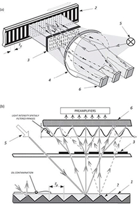
Fig. 7.4. Interferential measuring: (a) photoelectronic scanning, (b) optical filtering principle. 1 — scale, 2 — scale facets, 3 — phase gratings (readhead window), 4 — condenser lens, 5 — oblique illumination from LED, 6 — photodetectors.
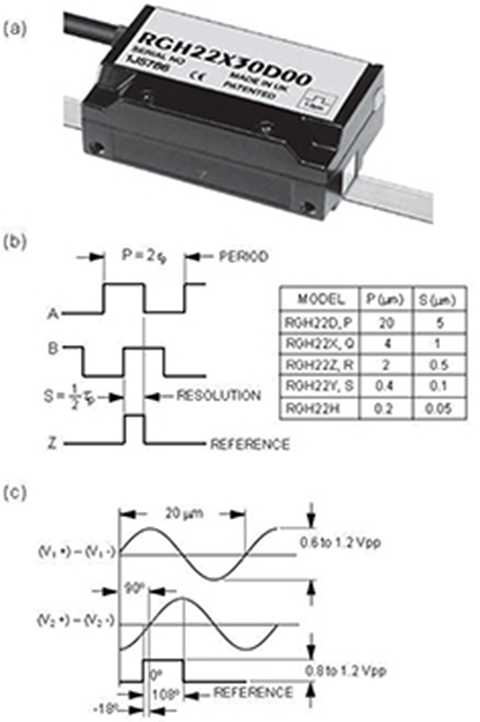
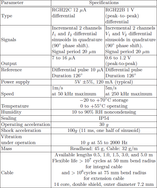
Fig. 7.5. Incremental readhead manufactured by Renishaw: (a) RGH22X readhead, (b) incremental 2 channels A and B in quadrature produced by digital readhead type, (c) incremental 2 channels V1 and V2 differential sinusoids in quadrature produced by analog readhead type. Courtesy of Renishaw plc, Gloucestershire, UK.
For digital output readheads, the recommended counterclock frequency for a given traversing speed is
where vtr is the traversing speed, sr is the readhead resolution, f is the counterclock frequency of interpolation electronics, and ksf is the safety factor, typically ksf = 4. If vtr is in m/s and sr is in μm, the counterclock frequency f is in MHz.
In less demanding applications that do not require high resolution (e.g., material handling or distribution centers), the parts location is defined by simple optical encoders rather than sophisticated scanning interferometers for both simplicity and cost reduction. In that case, the positioning relies on the counting of the square pulse sequence. The pulses are produced by the optical sensor positioned directly across the light source separated by a linear array of alternating transparent and opaque windows (Fig. 7.6). As the light source and detector (or alternatively, the window array strip) move, the output signal from the detector is switched sequentially ON and OFF. Addition of a second light source and detector set affords determination of movement direction. For systems with long travel displacements, a third light source and sensor set equipped with incremental encoders is typically utilized to indicate markers distributed along the track. Without these road markers, it is difficult to define an absolute position along the track. The disadvantage of this approach, however, is that the incremental encoders are vulnerable to power interrupts, noise, and contamination buildup, resulting in erroneous position information. Therefore, the need for these road markers and associated external counters required for determination of the absolute position between the markers constitute a major drawback of incremental encoders.
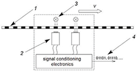
Fig. 7.6. Simplified incremental optical encoder arrangement. 1 — scale grating, 2 — detector ON/OFF, 3 — light source, 4 — counting bits.
Specifications of incremental self-adhesive scale RGS20-S produced by Renishaw plc, Gloucestershire, UK, is shown in Table 7.1. Dimensions of similar scale RGSZ20-S are shown in Fig. 7.7. Specifications of analog and digital readheads RGH series used in conjunction with RGS-S tape are presented in Table 7.2 and Table 7.3. The edge separation characteristics typical of digital readheads are shown in Fig. 7.8.
The optical readhead working with reflective scale of an incremental optical encoder is shown in Fig. 7.9.
The commonly used scale RGS20-S and one of the RGH22 series read-heads (Fig. 7.10) comprise the RG2 system, i.e., non-contact, optical encoder designed for position feedback solutions (Renishaw). The readhead can be chosen with either sinusoidal or square wave output. The selected type depends on the application, electrical interfacing, and required resolution. Typically, the RG2 encoders are employed in‘ linear motor-driven machines such as tool presetters, measuring and layout equipment, and other high-speed systems in which interpolation is provided by subsequent electronics. In the environments subjected to severe radio frequency interference (RFI), the RGH22B readhead with analog differential output voltage is preferred to the RGH22C model having the output current signal (Fig. 7.10).
Table 7.1. Self-adhesive scale RGS20-S for RG2 encoder system manufactured by Renishaw plc, Gloucestershire, UK
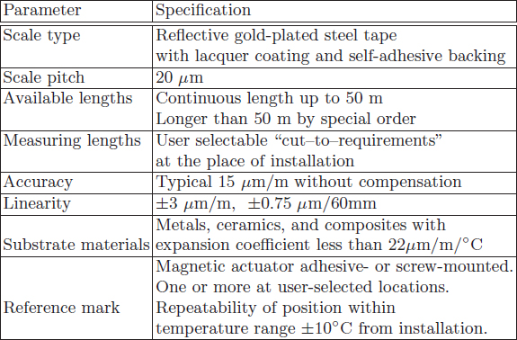

Fig. 7.7. Dimensions of RGSZ20-S scale and associated components. Courtesy of Renishaw plc, Gloucestershire, UK.

Fig. 7.8. RGH digital readheads characteristics: (a) edge separation, (b) recommended clock frequencies. Courtesy of Renishaw plc, Gloucestershire, UK.

Fig. 7.9. Readhead and reflective scale arrangement on the positioning stage with a linear motor. Photo courtesy of United Technologies Research Center, East Hartford, CT, USA.
Table 7.2. Analog readheads manufactured by Renishaw plc, Gloucestershire, UK
The x-y motion stages applied in clean-room environments, e.g., semiconductor industry or ultra-precision machine tools such as grinders for ferrite components and diamond lathes for optics, are equipped with integrated two-coordinate encoders. The incremental x-y encoder contains a 2D phase-grating structure on a glass substrate (Fig. 7.11). Specifications of the two-coordinate PP 281 R encoder manufactured by Heidenhain, GmbH, Traunreut, Germany, are listed in Table 7.4. The measurement in a plane is possible through an interferential scanning method. Two reference marks, one in each measurement direction, serve to define accurately the zero positions. The 8 μm grating period with fine interpolation and high uniformity of scanning is capable of 10 nm resolution.
Table 7.3. Specifications of digital readhead manufactured by Renishaw plc, Gloucestershire, UK

Table 7.4. Specifications of PP 281 R two-coordinate incremental encoder manufactured by Heidenhain, GmbH, Traunreut, Germany.
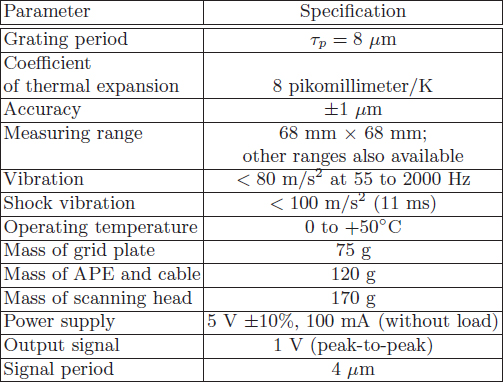
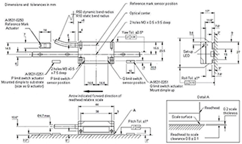
Fig. 7.10. Dimensions of the analog readhead RGH. Courtesy of Renishaw plc, Gloucestershire, UK.

Fig. 7.11. Two-coordinate incremental encoder PP281R. Photo courtesy of Heidenhain, GmbH, Traunreut, Germany.
7.1.2 Absolute Encoders
The obvious method of measuring linear position, velocity, or both is conversion of linear movement into rotary motion. The rotation is measured by angle sensors also known as rotary shaft encoders, analog multiturn shaft encoders, and absolute angle encoders. The operation principle of the rope-actuated linear position transducer, often referred to as cable extension transducer, yo-yo pot or string pot is illustrated in Fig. 7.12.

Fig. 7.12. Cable extension transducer. 1 — base, 2 — capstan, 3 — sensor, 4 — stainless steel wire rope, 5 — tension spring.
The transducer is fixed with the extensible wire rope attached to a movable object. As a result of object movement, the rope extends, rotating an internal transducer capstan. The sensing device then generates an electrical output signal proportional to the wire rope extension and/or to its velocity. The tension and retraction of the wire rope is achieved by an internal torsion spring mechanism. The sensing device may be a precision potentiometer, digital encoder, or a tachometer for velocity measurement. Liner position transducers proved to be a successful approach in a multitude of applications. With relatively non-critical alignment requirements, compact size, and ease of installation, these wire-rope-actuated transducers provide an extremely cost-effective method providing linear displacement feedback. Five different series of transducers manufactured by UniMeasure Inc., Corvallis, OR, USA are shown in Fig. 7.13.
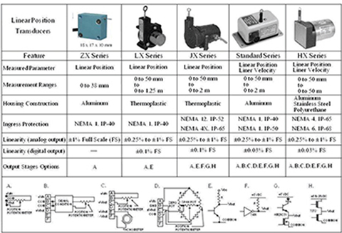
Fig. 7.13. Linear position cable extension transducers produced by UniMeasure Inc., Corvallis, OR, USA.
Typically, absolute encoders are utilized in the devices inactive for long periods of time or moving at low speeds. They are also applied to systems where linear position must be maintained regardless of power interruptions, or where safe and failure-free operation is required. Primarily, machine tools and robotics applications make use of absolute position encoders. These devices supply a whole output word with unique binary code pattern representing each position. This code is derived from independent tracks on the linear scale detected by individual photodetectors. The output from these detectors would then be high or low depending on the code pattern read off the linear scale for the particular position. Absolute encoders are similar to incremental devices; however, they contain more sensors. The overall complexity depends on the generated size of the word. The longer the logic word, the more complex and expensive the system. For each bit in the output signal, the encoder uses one track of the code scale. Therefore, a 10 bit encoder has 10 tracks to detect the light passing through them. For higher number of tracks, it may be necessary to use multiple sources of light to assure an adequate illumination. The principle of operation of the linear absolute encoder is illustrated in Fig. 7.14. Although the information read from data tracks can be converted into position signals using many different codes, natural binary code (NBC), gray, gray excess, and binary coded decimal (BCD) codes are most common.
The NBC derives the numerical value from exponents with base 2. For example, the number 179 is expressed as 1 × 27 + 0 × 26 + 1 × 25 + 1 × 24 + 0 × 23 + 0 × 22 + 1 × 21 + 1 × 20. In other words, the NBC value for 179 is 10110011.
The binary code is a polystrophic code characterized by multiple bit changes [187]. It requires many bit transitions simultaneously, e.g., counting from 127 to 128 in NBC requires simultaneous transition of 8 bits from 01111111 binary to 10000000 binary. In a practical electronic circuitry, all of these bits cannot be changed at precisely the same time. There is some delay within individual bit transitions. Ambiguity in the simultaneous bit changes, imperfection in the readhead mechanical installation, hysteresis and noise comprise only a few factors that affect the accuracy of the position detection. The potential error in the reading of the most significant bit can result in 180° feedback signal error.
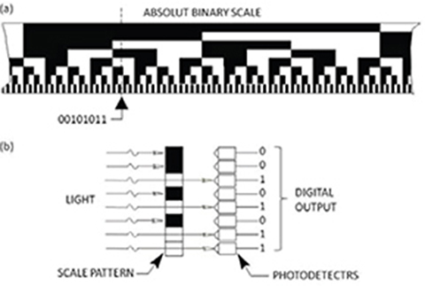
Fig. 7.14. Principle of operation of an absolute encoder: (a) absolute binary scale, (b) detection of bits.
More sophisticated scanning methods are used in modern absolute-position encoders. Two of them, the V-scan and the U-scan, allow for reliable simultaneous bit transitions. In the V-scan method, the sensors are positioned in the V-shape arrangement in two sensor banks (Fig. 7.15). Such a distribution makes room for error tolerances in the encoder system. The less significant bit is used to define in which direction the scale is moving, i.e., what kind of transition is performed (high–low or low–high).
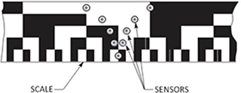
Fig. 7.15. Arrangement of sensors in V-scan method.
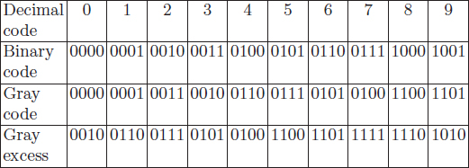
Another nonambiguous method is the gray code, particularly well suited to optical encoders. In this monostropic code, only two neighboring position values differ in exactly one binary digit, i.e. only one track changes at a time. This limits any decision during edge transition to plus or minus one count. Therefore, the maximum error when moving from one position to the next is 1/4 of the grating period of the finest track.
The gray excess code consists of a section from the middle of the gray code pattern. This permits a position value other than 2 and yet remains a unit-distance code (monostropic). An example of the gray excess code is: 4-bits of gray code provide 16 absolute position values, and to solve 10 positions, the first and last 3 values are omitted from the graduation pattern to produce the 10–excess–3 gray code. In the end, these codes (gray code, gray excess code, or any other appropriate code) are converted by the subsequent electronics (microprocessor) into the NBC. Differences between the binary and gray codes are shown in Table 7.5.
The application of absolute encoder scales to industrial linear motion systems characterized by extended single axis length (several tens of meters) typical of packaging, automation, and assembly lines is hindered by insufficient step resolution. For example, the scale with 12 tracks can generate 12-bit position information. This translates to 4096 unique encodings per scale length, providing approximately 250 μm resolution for 1 m of travel distance. In some cases, this is insufficient. An increase in the number of tracks can overcome this problem, but it results in higher complexity and costs of the encoder system. In practice, the total travel distance is subdivided into sections instead. Each section has the same absolute linear scale. To detect which section is actually scanned, the encoders use distance coded reference mark (DCRM). The distance coding is created by multiple reference marks individually spaced according to a specific mathematical algorithm. The span between every other reference mark, however, remains constant. The information as to which section is being sampled is calculated after traversing two successive reference marks. Rather than scanning the entire scale length, this method can reduce the search interval to 100 mm or less. Moreover, the DCRM scale system enables quick recovery of position information after power interruption or system shutdown. The absolute position is established without a need to traverse the entire scale [179]. The maximum length of coded scale and minimum traversed distance depend on the basic increment κsp, representing the distance between odd reference marks.
Table 7.5. Decimal, binary, gray, and gray excess codes
The value of κsp must be divisible by 2 times the grating scale τp (i.e. κsp/(2τp) with no remainder). With application of magnetic encoders, the scale grating τp is equal to the pole pitch of the magnetic tape. The maximum codable length Lmax allowing absolute position determination is calculated from
This is illustrated in Fig. 7.16 showing how the reference marks are distributed along the scale. The absolute position of the first traversed reference mark n is calculated according to the following formula [85]:
where Δn is a number of signal periods between two successively traversed reference marks, k is a basic spacing expressed in number of signal periods, k = κsp/τp. This formula yields n, a number of signal periods between the first mark on the scale (scale beginning) and the first traversed reference mark. The operator “sign” returns 0 if argument equals 0, 1 if argument is greater than 0, and −1 otherwise. The traversed direction is accounted for by a proper choice of sign in the second term of eqn (7.3). The “−” sign represents forward motion, while the “+” sign stands for backward motion.

Fig. 7.16. Representation of an incremental scale with distance-coded reference mark.
In motion systems where safety and failure-free operation are not a priority, incremental rather than the absolute optical scales can be employed for distance-coded reference marks. Here, the absolute position is determined by counting the number of steps from each reference mark. In case of power interruption, however, the position information may be lost and can only be recovered by traversing at least two neighboring reference marks.
Linear encoders used in the metal cutting industry, i.e., LBM drives for machine tool tables, must meet the following requirements [84]:
High counting accuracy at high speeds, e.g., from 0.1 to 0.25 m/s in milling of gray-cast iron and aluminum (this translates into wide frequency range of position loop-control and, therefore, fast feed-forward control).
High acceleration capability, typically from 10 to 40 m/s2 and even higher.
High maximum rapid-travel speeds, typically from 1 to 1.5 m/s, sometimes even 2 m/s.
Manufacturers have developed two types of constructions that can meet these requirements: (a) exposed, and (b) sealed encoders. Exposed encoders are recommended in clean environments without a danger to contaminate the optics. However, in machines either completely encapsulated or using coolant and/or lubricant, sealed encoders are preferred. The advantage of the sealed system lies in the reduction of requirements for finishing the mounting surface. Furthermore, sealed linear encoders are characterized by simple mounting and higher protection rating. On the other hand, the advantages of exposed encoders include higher traversing speed, no friction, and better accuracy. Therefore, exposed encoders most often find applications in precision machines, measuring systems, and production equipment for the semiconductor industry. On the other hand, sealed linear encoders are widely utilized in metal-cutting machines.
Table 7.6. Sealed absolute linear encoder LC 181 manufactured by Heidenhain, GmbH, Traunreut, Germany
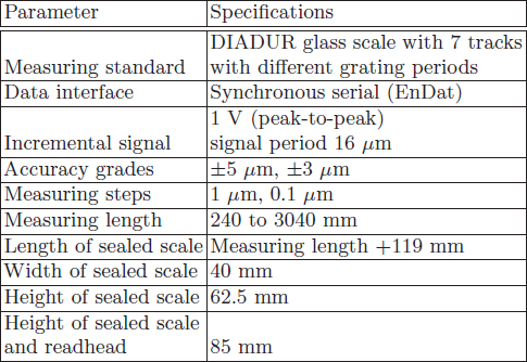
The Heidenhain LC 181 sealed absolute position encoder data is shown in Table 7.6. It generates the absolute position value from seven incremental tracks. The grating periods of the tracks differ in a manner that makes it possible to evaluate the measuring signals of all seven tracks. This allows identification of any location on the scale within the measuring length of 3 m. In addition to the absolute position information, the LC 181 encoder provides sinusoidal incremental signal with its period of 16 μm at 1 V (peak-to-peak).
7.1.3 Data Matrix Code Identification and Positioning System
Optical laser and digital photo technologies are now widely applied in many areas of industrial production providing accurate information about the flow of goods and commodities. Depending on application, this might include determining the position of moving entities (e.g., work pieces, tool carriers), monitoring a car on a suspended rail system (e.g., in warehouses, distribution centers), or monitoring a conveyer (e.g., in warehouses, production facilities). The most advanced position encoding/identification system suitable for long travel-path applications is data matrix coding [169]. These systems allow for identification and synchronization of many objects transported over distances exceeding 300 m with the precision on the order of a fraction of a millimeter. Complex and extensive motion systems containing turns, junctions, and gradients, e.g., crane positioning, elevators, galvanization stations, or studio technology constitute the primary target for data matrix installations.
The data matrix technology is based on scanning of red light reflection from a coded label akin to the barcode identification systems. The main difference is that the barcode is an one-dimensional code. Meanwhile, the data matrix code is a two-dimensional representation of encoded information with capacity up to 1.5 kB condensed onto a very small footprint area. The data matrix codes can be printed directly on plastic or metal substrates. The bit code with built-in error correction is set in a chessboard fashion. A data matrix reader captures the code in a image, evaluates it internally, and sends the decoded information as a text command to the controller via Ethernet. This enables high passing speeds and allows code readout even when the information is partially lost. An example data matrix reader, ODT-MAC 400 produced by Pepperl+Fuchs GmbH, Manneheim, Germany, is capable of reading objects at speeds up to 20 m/s and at frequencies up to 60 scans/s. Detailed parameters of MAC 400 readers series are specified in Table 7.7. The exemplary application of data matrix system is illustrated in Fig. 7.17.
Table 7.7. Data matrix reader MAC400 manufactured by Papperl+Fuchs, GmbH, Mannheim, Germany.
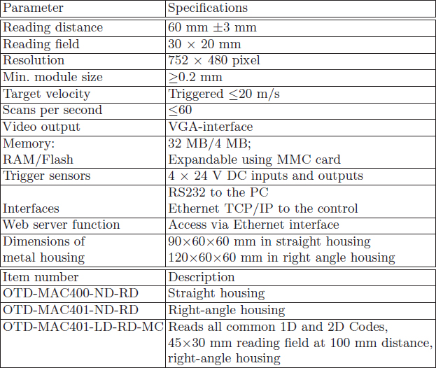
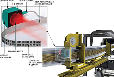
Fig. 7.17. Application of data matrix positioning system. Courtesy of Pepperl+Fuchs, GmbH, Mannheim, Germany.
7.2 Linear Magnetic Encoders
7.2.1 Construction
As compared with optical sensors, their magnetic counterparts are characterized by simplicity, reduced sensitivity to contamination, robustness, and low cost. Magnetic sensors can work in the presence of heavy liquid and chip buildup. Made out of metal, they can withstand more severe vibrations and are perceived to be more reliable. In addition, these devices have lower power requirements, good performance characteristics, and are well suited for large-volume manufacturing technology.
Magnetic encoders utilize magnetoresistive (MR) sensing elements and magnetically salient targets. The magnetically salient target is a long, alternatively magnetized ruler. The MR elements (sensors) change their resistance under the influence of magnetic flux density and can sense flux densities above 0.005 T [187]. The principle of operation of the magnetic linear encoder with the MR sensors is explained in Fig. 7.18. The MR sensor resistance changes approximately ±1.6% as the magnetic field excited by the passing salient target changes its polarity. Four sensors are electrically connected to a resistive bridge polarized by 5 V d.c. source. The bridge output voltage varies sinusoidally within the amplitude of 0.08 V (peak-to-peak) reflecting changes of sensor resistances. The two magnetic poles affect the sensors in the same way but with opposite polarity. Therefore, when the alternatively magnetized ruler moves one pole pitch τp, the output signal will complete one cycle. Sine and cosine signals are produced as the sensors traverse the scale. These analogue signals are interpolated internally to produce the resolution up to 4 μm.
Magnetic encoders employing MR sensors are capable of producing output signals with frequencies up to 200 kHz. High frequency response requires very high resolution, which is a function of the air gap size. The smaller the gap, the higher the resolution. This gap size should be approximately 80% of the pole pitch. For example, if a motion system requires the resolution of 0.05 mm (20 kHz frequency with 1 m/s linear speed), the encoder with 4 × interpolation should contain the magnetic target with 0.2 mm pole pitch. The air gap in such a system is about 0.15 mm.

Fig. 7.18. Magnetic encoder with MR sensors.
Sensing elements and magnetically salient targets with stick-on reference marks are typically supplied as separate components. The scale can be supplied on a reel or cut to a specific length and protected by a nonmagnetic stainless cover strip. Occasionally, motion system hardware may be adopted by the end user to serve as a long salient target. In such a system, air gaps between sensors and the target are usually on the order of a few millimeters. The magnetoresistive (MR) linear magnetic encoders, produced by Merilna Tehnika, Ljubljana-Dobrunje, Slovenia, are presented in Fig. 7.19, [180].
In magnetic encoders with large air gaps the Hall elements are more suitable than MR sensors. These are true solid-state devices with good operating temperature limits, typically from −40 to 150 °C, long life expectation (20 billion operations), and which can work at zero speeds. The linear (analog) Hall element has a wide range of output signals (from 1.5 to 4.5 V) and a reasonable frequency response (100 kHz). Its output voltage is
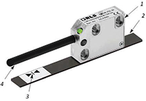
Fig. 7.19. RLS incremental magnetic encoder. 1 — readhead, 2 — magnetic scale, 3 — stick-on reference mark, 4 — cable. Photo courtesy of RLS Merilna Tehnika, Ljubljana-Dobrunje, Slovenia.
where Ic is the applied current, B sin θ represents the component of the magnetic flux density vector perpendicular to the current path, θ is the angle between the magnetic flux density vector and the Hall element surface, δ is the thickness of the Hall element, and kH is Hall constant (m3/C).
Specifications of a typical Hall effect sensor are listed in Table 7.8. This sensor is used to scan moving electromagnetic objects, preferably toothed ferromagnetic racks [130].
Table 7.8. Specifications of the IHRM 12P15001 sensor employing magnetically biased Hall element manufactured by BEI Corporation, Industrial Encoder Division, Tustin, CA, USA

Encoder systems with Hall effect devices are arranged in a different way than those comprising MR elements. Hall sensors are typically placed between a moving, magnetically salient target, e.g., ferromagnetic ruler with teeth, and a bias PM that excites the magnetic field. In the case of low resolution of positioning systems, a long flexible magnetic strip distributed along the motion track serves as the magnetically salient target. This strip is made out of ferrite material or low-energy NdFeB PMs mixed with rubber, and is usually alternatively magnetized, i.e., N, S, …, N, S with pole pitch of a few millimeters. The alternatively magnetized flexible strip permits achieving repeatability up to ±5 μm (1.22 μm resolution) with 4096× multiplier (electronic circuit). The relative position is determined by counting the number of poles or target saliencies (steel teeth) moving through the sensor, while the speed is obtained from the frequency at which they pass. Meanwhile, the movement direction is obtained from the relative timing of two sensors in the quadrature with target saliency. This flexible-strip-based linear encoder is used in LEU, LEM and LZ series linear motors with inner air-cored armature winding manufactured by Anorad, now a branch of Rockwell Automation [12].
In linear motors utilized for propulsion with an array of magnetic poles N, S, …, N, S and short pole pitch, the installation of an additional magnetic strip for the encoder is not necessary. Encoder sensors are located near the surface of the guideway, and the field produced by PMs is used as the magnetic target.

Fig. 7.20. Noise canceling magnetic sensors: (a) PM reaction rail, (b) ferromagnetic reaction rail with saliency. S1, S3 — antiphase sensors, S2 — noise-canceling sensor.
7.2.2 Noise Cancelation
One of the disadvantages of linear magnetic encoders is their sensitivity to external magnetic fields and temperature changes. Sometimes, the magnetic noise can exceed the sensor-generated signal up to one order of magnitude. Therefore, noise cancelation techniques aimed at suppression of unwanted disturbance signals are required.
One of the simple noise cancelation methods is based on an array of three magnetic sensors [P70]. Two of them are situated half of the magnetic period apart (in antiphase relationship, i.e., 180° out–of–phase), while the third sensor is placed between the two remaining. The three-sensor array is shown in Fig. 7.20.
The individual sensor output signal is a function of the magnetic flux density created by passing magnetic targets and the ambient noise of magnetic origin. For magnetic poles of alternative polarity (Fig. 7.20a), the three sensor output signals can be expressed as
where x is the pole or saliency position in the direction of motion, and N is the noise signal. Quadrature positions s1c and s2c are derived from the three sensor signals s1, s2, and s3 as follows:
and
The sensor output quadrature signals s1c and s2c are digitized for the complete noise cancelation enhancement. In some applications, the noise N depends on the position of the magnetic pole within the strip along the reaction rail. This results in incomplete noise cancelation. However, digitization with zero-crossing detection occurring at points of geometrical symmetry will fully cancel the noise signals. Fig. 7.21 depicts the sensor output signal with resulting zero-crossing digitization.

Fig. 7.21. Quadrature sensor output signals s1c and s2c digitized by sensing zero-crossings.
7.2.3 Signal Interpolation Process
The interpolation is a process of an encoder signal subdivision into phase-shifted copies. It can be applied to sinusoidal outputs in the quadrature only. For example, the transistor–transistor logic (TTL) signals cannot be interpolated. To enhance the resolution effectiveness, i.e., the overall accuracy, the interpolated signals are recombined in electronic circuitry.
The sinusoidal signals formed by the incremental encoders are processed by the digitizing electronic units. These are often incorporated into a numerical motion controller and enclosed in a separate housing. Three of the commonly used interpolation methods, i.e., (a) analog–digital interpolation using resistor networks, (b) digital interpolation with look-up and tracking counter, and (c) digital interpolation with arc-tangent calculator, have successfully been applied to the Heidenhain, GmbH encoders.
The first method makes use of the trigonometric identity sin(α + β) = sin α cos β + cos α sin β to develop the phase-shifted copies of the original signals.
The encoder LS 774/LS 774C manufactured by Heidenhain, GmbH is based on the analog–digital conversion with 5-fold interpolation (the so called 5 × interpolator). The scanning signals s1c and s2c are amplified and interpolated in the resistor network that generates collateral phase-shifted signals by using vector algebra. The 5-fold interpolation process is shown in Fig. 7.22. Ten signals are produced with a phase shift ranging from 0° to 162° electrical. After conversion to the quadrature, these signals are combined into two square-wave trains by exclusive-OR (XOR) gates. The trains of impulses have frequency five times greater than that of the scanning input signals and are phase-shifted by quarter of the period. Each edge of the signals S1 and S2 can be used as a counting pulse within one period. The reference pulse S0 is gated between the two successive edges of S1 and S2. The 20 μm grating period of the encoder, which combines 5-fold interpolation with 4-fold electronic evaluation, is capable of achieving 1 μm measuring step. A similar process can be used for 10- or 25-fold interpolation that results in 1/40 or 1/100 measuring step of the grating period.
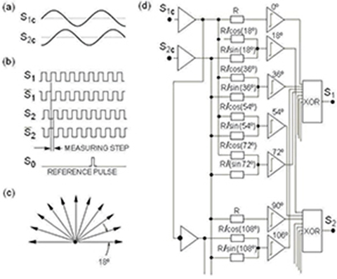
Fig. 7.22. Interpolation process with resistor network: (a) scanning signals, (b) measuring signals after 5-fold interpolation and digitization, (c) signal vectors diagram, (d) electronic circuit.
In interpolation processes utilizing higher subdivisions (50-fold and above), digital methods are required. Two scanning signals are first amplified, then quantified in the sample-and-hold circuitry, and finally digitized into regular intervals in the A/D converter. These digitized voltages define a single address (row and column) in a lookup table describing an instantaneous position (Fig. 7.23a). The actual position is compared with the value determined in the previous cycle that is stored in a tracking counter. The tracking counter produces incremental square-wave signals (0° and 90°) from the differences between previous and current positions. The lookup table interpolation method is used in the EXE 650 (50-fold interpolation) and EXE 660 (100-fold interpolation) encoders manufactured by Heidenhain, GmbH.
The most advanced interpolators use microprocessor technology. Fig. 7.23b illustrates the digital interpolation process employing an arctangent calculator. The microprocessor calculates the tangent S1/S2 from two digitized input voltages. The corresponding angle value (arctangent), which indicates the position within one signal period, is derived from the table stored in EPROM. The analog input signals s1c and s2c are simultaneously converted into quadrature waveforms, and signal periods are determined. The actual position is derived from the evaluated period and the calculated angle. Finally, to compensate for system errors, appropriate correction values are read from the table stored in the RAM. After the error correction, the digital signal is transmitted to the motion control unit.

Fig. 7.23. Digital interpolation methods: (a) using lookup table and tracking counter, (b) using microprocessor to compute arctangent.
7.2.4 Transmission of Speed and Position Signals
The speed and position control systems are limited by the pulse per meter counts and the maximum linear speed/frequency response rate, which depends on
mechanically permissible traversing speed,
minimum possible edge separation of the square-wave output signals S1 and S2,
maximum input frequency of the interpolating and the digitizing electronics.
The maximum traversing speed
depends on the maximum input frequency f of the interpolation and digitizing electronics and the scale grating period τp. If f is in kHz, and τp is in μm, the speed vtr is in mm/s. An example of the relationship between maximum traversing speed and the grating period at various maximum permissible input frequencies is illustrated in Fig. 7.24.

Fig. 7.24. Maximum permissible input frequencies for EXE interpolation unit. Courtesy of Heidenhain, GmbH, Traunreut, Germany.
The encoder signal is subdivided in subsequent electronics. The subdivision factor should remain in reasonable proportion to the accuracy of the encoder. For example, the subdivision factor of 1024 applied to the 10 μm or 40 μm signal period gives the resolution of approximately 10 nm and 40 nm, respectively.
Feed drives of machine tools can reach linear speeds over 2 m/s, while the handling equipment can reach over 5 m/s. It can be calculated that the velocity of 1 m/s and measuring step of 0.1 μm (after a 4-fold evaluation) result in the input frequency of 2.5 MHz. Owing to large distances separating the encoder and the processing electronics (up to 50 m), the interpolating and digitizing circuit is often connected as a separate unit between them. For signals with frequencies above 1 MHz, short cables need to be employed in order to preserve good transmission quality. Therefore, high-speed motion systems utilize encoders containing interpolation and digitizing circuits. If the high-frequency transmission signal is unavoidable, e.g., in the system with high traversing speed and small measuring steps, a linear encoder with sinusoidal output signals should be used. This sinusoidal signal should be 1 V (peak-to-peak) at the cutoff frequency of 200 kHz with amplitude of −3 dB. In this case, the cable length can reach 150 m.
Low traversing speed with high uniformity of motion requirement sets another limit for the measurement system. To maintain adequately uniform speed, a resolution of 0.1 μm and higher may be required.

Fig. 7.25. Edge separation diagram applied to non-clock EXE interpolation unit. Courtesy of Heidenhain, GmbH, Traunreut, Germany.
In general, the control electronics limits the minimum edge separation for square-wave output signals. The relationship between input frequency f and the edge separation a for a given interpolation factor is shown in Fig. 7.25. The input frequency f can be found from eqn (7.10).
7.2.5 LVDT Linear Position Sensors
The Linear Variable Differential Transducer (LVDT) is a common electromechanical converter producing an electrical signal in response to rectilinear motion [137]. This linear position sensor is capable of measuring translation from a fraction of a micrometer to approximately half a meter.
The internal structure of the LVD transducer (Fig. 7.26) consists of primary winding centered between two identical secondary windings equidistant from the center. All three coils are wound on a single hollow tube made of thermally stable glass reinforced polymer. Typically, the coils assembly is wrapped in a high-permeability magnetic shielding and secured in the cylindrical stainless steel housing. This coil assembly constitutes the stationary element of the position sensor. The sensor’s translating member is made up of the ferromagnetic cylinder core moving axially within a hollow bore of the coil assembly. During operation, the primary coil is excited by an a.c. current of appropriate frequency and magnitude. The transducer’s electrical output signal is an alternating voltage between the two secondary coils. The magnitude of the output a.c. voltage depends on the axial position of the core within the coil assembly. This a.c. voltage is converted by suitable electronic circuitry to the high-level d.c. signal. The LVDT’s functioning principles are illustrated in Fig. 7.27.
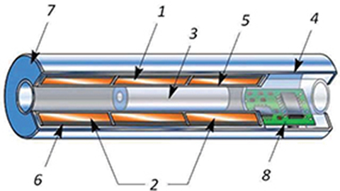
Fig. 7.26. Cross-section of LVDT transducer. Courtesy of Macro SensorsTM, Pennsauken, NJ, USA. 1 — primary winding, 2 — secondary windings, 3 — core, 4 — magnetic shell, 5 — coil form, 6 — epoxy encapsulation, 7 — stainless steel housing and end caps, 8 — signal-conditioning electronics module.
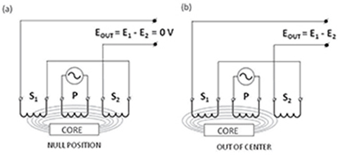
Fig. 7.27. Principle of generating output signals in the LVDT linear transducer.
The primary coil P is energized by an a.c. current of constant amplitude. This generates magnetic flux through the ferromagnetic C-shaped core and mutually coupling the secondary windings S1 and S2. When the core is located exactly midway between S1 and S2 (Fig. 7.27a), the mutual inductances between the primary coil P and both the secondary coils S1 and S2 are the same. Consequently, the voltages E1 and E2 induced in the windings are equal to each other. At this null point (also known as the reference position), the differential voltage output (E1 − E2) equals zero. As the core moves closer to one of the secondary windings, it generates a stronger magnetic coupling between the two. Subsequently, the induced voltages E1 and E2 are not the same, and the sensor output voltage is nonzero. The differential signal magnitude (E1 −E2) is proportional to the core distance from the reference position as illustrated in Fig. 7.28a. The value of Eout at the maximum core displacement is on the order of several rms V. It depends on the amplitude of the primary excitation voltage and the sensitivity of the LVDT structure. The Eout phase angle referenced to the primary excitation voltage remains constant until the core center passes the reference position, at which point the phase angle changes abruptly by 180° (Fig. 7.28b). This phase shift is used to define the motion direction.
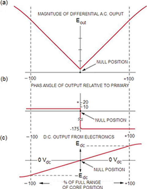
Fig. 7.28. Output characteristics of an LVDT position sensor: (a) magnitude of differential a.c. output as a function of the core position, (b) phase of the output a.c. signal relative to the primary coil excitation P, (c) electronic conditioning unit d.c. output signal.

Fig. 7.29. Hermetically sealed frictionless LVDT position sensors LP 750 series, Macro SensorsTM.
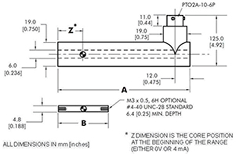
Fig. 7.30. Geometrical details of LP 750 series sensors.
Fig. 7.29, Fig. 7.30, and Table 7.9 show specifications of commercial LVDT series, manufactured by Macro SensorsTM, Pennsauken, NJ, USA [129].
Table 7.9. Specifications of LP 750 series LVDTs manufactured by Macro SensorsTM, Pennsauken, NJ, USA

Examples
Example 7.1
An application of linear encoder with scale grating τp = 5 mm requires measurement of position along the 15 m track length. Calculate the minimum basic spacing k between odd reference marks warranting recovery of the unique absolute position with application of DCRM over the entire axis length. Moreover, determine the scanning head position after power interruption if the head was traversing in a backward direction and 59 signal periods were counted between two successive reference marks.
Solution
The millimeter length units are used throughout the following calculations. The basic increment κsp is found by rearranging eqn (7.2) and solving the resultant quadratic equation
Substituting known quantities
There exists only one proper solution to this quadratic equation κsp1 = 397.43 mm. However, the basic increment must be dividable by two times the scale grating without remainder, (2τp = 10). The correct value of κsp is found using function ceil [κsp1/(2τp)] that returns the last integer equal to or greater than the argument
The actual codable length according to eqn (7.2) for κsp = 400 mm is
The position of readhead after power recovering is calculated using eqn (7.3). First, the basic increment κsp = 400 mm should be converted into basic spacing k counted in the number of signal periods τp:
With +1 for backward traversing direction, Δn = 59, and k = 80 stated in (7.3), the absolute position of the first traversed reference mark is
counted from the first reference mark on the scale, i.e. from the position designator. Finally, the absolute position of the first traversed reference mark counted from the scale beginning is (Fig. 7.16).

Fig. 7.31. Schematic of the analyzed LVDT. Example 7.2.

Fig. 7.32. Signal output linearity. Example 7.2.
Example 7.2
The schematic and dimensions of an exemplary LVDT used for conversion of linear position to voltage signal are specified in Fig. 7.31. The core is shown positioned at the null point. The full measurement range is 25.4 mm. Determine the linearity of the output signal as a function of displacement.
Solution
The examination is conducted using the Magnet Infolytica FEM package [54]. Even though the linear differential transformer uses alternating current supplied to the primary coil 0, the problem is modeled as a static because the solution does not depend on eddy currents in the core. The output voltage is a function of the coil 1 and 2 flux linkage, and can be obtained from the static field solution. The differential flux linkage between the sensing coils is calculated at successive positions of the core, starting at position x = 0 mm and ending with the core shifted by 25.4 mm to the right. While the output signal linearity does not depend on the number of turns within the coils, its magnitude does. Therefore, to simplify the analysis and obtain higher values of the differential linkage flux, n0 = 5000 and n1 = n2 = 3000, the number of turns have been assumed for the primary and secondary coils, respectively. Within the framework of the FEM model, the secondary coils have been connected in opposition to each other. Thus, the start face of coil 2 was connected to the end face of coil 1. To keep the current density below 2.5 A/mm2) (coil’s thermal capability), 50 mA primary current was chosen. The parametric FEM model with 2D rotational geometry was simulated for the following 18 core positions: 0, 0.4, 1.0, 2.0, 4.0, …, 20, 22, 23, 24, 25, 25.4 mm. All magnetic elements of the LVDT have been assumed to possess high and constant magnetic permeability, μr = 1000 (to avoid saturation in effect).
The flux linkage as a function of the core position for the FEM of Example 7.2 is illustrated in Fig. 7.32.