3 Theory of Linear Synchronous Motors

Search in book...
Toggle Font Controls
Create new playlist

Name your new playlist

Playlist description (optional)
Sign In

Email address

Password

Forgot Password?

or

Continue with Facebook

Continue with Google
Sign Up

Full Name

Email address

Confirm Email Address

Password

or

Continue with Facebook

Continue with Google

The time-space distribution of the magnetomotife force (MMF) of a symmetrical polyphase winding with distributed parameters fed with a balanced system of currents can be expressed as

$\begin{matrix} F (x, t) = \frac{N_{1} \sqrt{2} I_{a}}{π p} sin(ω t) Σ_{ν = 1}^{\infty} \frac{1}{ν} k_{w 1 ν} cos(ν \frac{π}{τ} x) \\ + \frac{N_{1} \sqrt{2} I_{a}}{π p} sin(ω t - \frac{1}{m_{1}} 2 π) \sum_{ν = 1}^{\infty} \frac{1}{ν} k_{w 1} \cos ν (\frac{π}{τ} x - \frac{1}{m_{1}} 2 π) + ... \\ + \frac{N_{1} \sqrt{2} I_{a}}{π p} sin(ω t - \frac{m_{1} - 1}{m_{1}} 2 π) \sum_{ν = 1}^{\infty} \frac{1}{ν} k_{w 1 ν} \cos ν (\frac{π}{τ} x - \frac{m_{1} - 1}{m_{1}} 2 π) \\ = \frac{1}{2} \sum_{ν = 1}^{\infty} F_{m ν} {sin [(ω t - ν \frac{π}{τ} X) + (ν - 1) \frac{2 π}{m_{1}}] \\ + \sin [(ω t + ν \frac{π}{τ} x) - (ν + 1) \frac{2 π}{m_{1}}]} \end{matrix} (3.1)$

where I_a is the armature phase current, m₁ is the number of phases, p is the number of pole pairs, N₁ is the number of series turns per phase, k_w1ν is the winding factor, ω = 2πf is the angular frequency, τ is the pole pitch, and

for the forward-traveling field

$\begin{matrix} ν = 2 m_{1} k + 1, & k = 0, 1, 2, 3, 4, 5, \dots \end{matrix} (3.2)$
for the backward-traveling field

$\begin{matrix} ν = 2 m_{1} k - 1, & k = 1, 2, 3, 4, 5 \dots \end{matrix} (3.3)$

The magnitude of the νth harmonics of the armature MMF is

$F_{m ν} = \frac{2 m_{1} \sqrt{2}}{π p} N_{1} I_{a} \frac{1}{ν} k_{w 1 ν} = m_{1} {[F_{m ν}]}_{m_{1} = 1} (3.4)$

where ${[F_{m v}]}_{m_{1} = 1}$ is the magnitude of the armature MMF of a single-phase winding. The winding factor for the higher-space harmonics ν > 1 is the product of the distribution factor, k_d1ν, and the pitch factor, k_p1ν, as given by eqns (2.48), (2.49), and (2.50) in Chapter 2. See also eqns (2.39), (2.40), and (2.41) given in Chapter 2, expressing k_w1ν = k_w1, k_d1ν = k_d1, and k_p1ν = k_p1 for ν = 1.

Assuming that ωt ∓ νπx/τ = 0, the linear synchronous speed of the νth harmonic wave of the MMF is

$v_{s ν} = \mp 2 f τ \frac{1}{ν} (3.5)$

For a three-phase winding, the time space distribution of the MMF is

$\begin{matrix} F (x, t) = \frac{1}{2} \sum_{ν = 1}^{\infty} F_{m ν} {sin [(ω t - \frac{π}{τ} x) + (ν - 1) \frac{2 π}{3}] \\ + \sin [(ω t + ν \frac{π}{τ} x) - (ν + 1) \frac{2 π}{3}]} \end{matrix} (3.6)$

For a three-phase winding and the fundamental harmonic ν = 1,

$F (x, t) = \frac{1}{2} F_{m} sin(ω t - \frac{π}{τ} x) (3.7)$

$F_{m} = \frac{2 m_{1} \sqrt{2}}{π p} N_{1} I_{a} k_{w 1} \approx 0.9 \frac{m_{1} N_{1} k_{w 1}}{p} I_{a} (3.8)$

the winding factor k_w1 = k_d1k_p1 is given by eqns (2.39), (2.40), and (2.41), and v_s = v_sν=1 is according to eqn (1.1).

The peak value of the armature line current density or specific electric loading is defined as the number of conductors (one turn consists of two conductors) in all phases 2m₁N₁ times the peak armature current $\sqrt{2} I_{a}$ divided by the armature stack length 2pτ, i.e.,

$A_{m} = \frac{m_{1} \sqrt{2} N_{1} I_{a}}{p τ} (3.9)$

3.1.2 Form Factors and Reaction Factors

The form factor of the excitation field is defined as the ratio of the amplitude of the first harmonic-to-maximum value of the air gap magnetic flux density, i.e.,

$k_{f} = \frac{B_{m g 1}}{B_{m g}} = \frac{4}{π} \sin \frac{α_{i} π}{2} (3.10)$

where α_i is the pole-shoe b_p to pole pitch τ ratio, i.e.,

$α_{i} = \frac{b_{p}}{τ} (3.11)$

The form factors of the armature reaction are defined as the ratios of the first harmonic amplitudes to maximum values of normal components of armature reaction magnetic flux densities in the d-axis and q-axis, respectively, i.e.,

$\begin{matrix} k_{f d} = \frac{B_{a d 1}}{B_{a d}} & k_{f q} = \frac{B_{a q 1}}{B_{a q}} \end{matrix} (3.12)$

The direct or d-axis is the center axis of the magnetic pole, while the quadrature or q-axis is the axis perpendicular (90° electrical) to the d-axis. The peak values of the first harmonics B_ad1 and B_aq1 of the armature magnetic flux density can be calculated as coefficients of Fourier series for ν = 1, i.e.,

$B_{a d 1} = \frac{4}{π} \int_{0}^{0.5 π} B (x) \cos x d x (3.13)$

$B_{a q 1} = \frac{4}{π} \int_{0}^{0.5 π} B (x) \sin x d x (3.14)$

For a salient-pole motor with electromagnetic excitation and the air gap g ≈ 0 (fringing effects neglected), the d- and q-axis form factors of the armature reaction are

$\begin{matrix} k_{f d} = \frac{α_{i} π + \sin α_{i} π}{π} & k_{f q} = \frac{α_{i} π - \sin α_{i} π}{π} \end{matrix} (3.15)$

For PM excitation systems, the form factors of the armature reaction are [70]

for surface PMs

$k_{f d} = k_{f q} = 1 (3.16)$
for buried magnets

$\begin{matrix} k_{f d} = \frac{4}{π} α_{i}^{2} \frac{1}{α_{i}^{2} - 1} \cos \frac{π}{2 α_{i}} & k_{f q} = \frac{1}{π} (α_{i} π - \sin α_{i} π) \end{matrix} (3.17)$

Formulae for k_fd and k_fq for inset type PMs and surface PMs with mild steel pole shoes are given in [66].

The reaction factors in the d- and q-axis are defined as

$\begin{matrix} k_{a d} = \frac{k_{f d}}{k_{f}} & k_{a q} = \frac{k_{f d}}{k_{f}} \end{matrix} (3.18)$

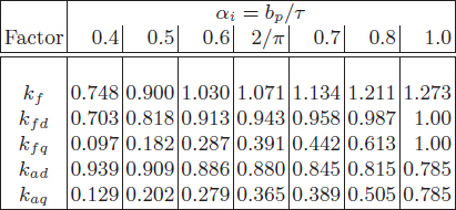
The form factors k_f, k_fd, and k_fq of the excitation field, and armature reaction and reaction factors k_ad and k_aq for salient-pole synchronous machines according to eqns (3.10), (3.15), and (3.18), are given in Table 3.1.

Table 3.1. Factors k_f, k_fd, k_fq, k_ad, and k_aq for salient-pole synchronous machines according to eqns (3.10), (3.15), and (3.18)

Images

Assuming g = 0, the equivalent d-axis field MMF (which produces the same fundamental wave flux as the armature-reaction MMF) is

$F_{a d} = k_{a d} F_{a d} = \frac{m_{1} \sqrt{2}}{π} \frac{N_{1} k_{w 1}}{p} k_{a d} I_{a} sinΨ (3.19)$

where I_a is the armature current, and Ψ is the angle between the phasor of the armature current I_a and the q-axis, i.e., I_ad = I_a sin Ψ. Similarly, the equivalent q-axis field MMF is

$F_{a q} = k_{a q} F_{a q} = \frac{m_{1} \sqrt{2}}{π} \frac{N_{1} k_{w 1}}{p} k_{a q} I_{a} cosΨ (3.20)$

where I_aq = I_a cos Ψ. In the theory of synchronous machines with electromagnetic excitation, the MMFs F_excd and F_excq are defined as the armature MMFs referred to the field excitation winding.

3.1.3 Synchronous Reactance

For a salient-pole synchronous machine, the d-axis and q-axis synchronous reactances are

$\begin{matrix} X_{s d} = X_{1} + X_{a d} & X_{s q} = X_{1} + X_{a q} \end{matrix} (3.21)$

where X₁ = 2πfL₁ is the armature leakage reactance according to eqn (2.32), X_ad is the d-axis armature reaction reactance, also called d-axis mutual reactance; and X_aq is the q-axis armature reaction reactance, also called q-axis mutual reactance. The reactance X_ad is sensitive to the saturation of the magnetic circuit, while the influence of the magnetic saturation on the reactance X_aq depends on the field excitation system design. In salient-pole synchronous machines with electromagnetic excitation, X_aq is practically independent of the magnetic saturation. Usually, X_sd > X_sq except for some PM synchronous machines.

The d-axis armature reaction reactance

$X_{a d} = k_{f d} X_{a} = 4 m_{1} μ_{0} f \frac{{(N_{1} k_{w 1})}^{2}}{π p} \frac{τ L_{i}}{g^{'}} k_{f d} (3.22)$

where μ_o is the magnetic permeability of free space, L_i is the effective length of the stator core, g ≈ k_Ck_satg + h_M/μ_rrec is the equivalent air gap in the d-axis, k_C is the Carter’s coefficient for the air gap according to eqn (2.44), k_sat > 1 is the saturation factor of the magnetic circuit, and

$X_{a} = 4 m_{1} μ_{0} f \frac{{(N_{1} k_{w 1})}^{2}}{π p} \frac{τ L_{i}}{g^{'}} (3.23)$

is the armature reaction reactance of a non-salient-pole (surface configuration of PMs) synchronous machine. Similarly, for the q-axis,

$X_{a q} = k_{f q} X_{a} = 4 m_{1} μ_{0} f \frac{{(N_{1} k_{w 1})}^{2}}{π p} \frac{τ L_{i}}{k_{C} k_{s a t q} g_{q}} k_{f q} (3.24)$

where g_q is the air gap in the q-axis. For salient-pole excitation systems, the saturation factor k_satq ≈ 1 since the q-axis armature reaction fluxes, closing through the large air spaces between the poles have insignificant effect on the magnetic saturation.

The leakage reactance X₁ consists of the slot, end-connection differential and tooth-top leakage reactances — see eqn (2.32). Only the slot and differential leakage reactances depend on the magnetic saturation due to leakage fields.

3.1.4 Voltage Induced

The no-load rms voltage induced (EMF) in one phase of the armature winding by the d.c. or PM excitation flux Φ_f is

$E_{f} = π \sqrt{2} f N_{1} k_{w 1} Φ_{f} (3.25)$

where N₁ is the number of the armature turns per phase, k_w1 is the armature winding coefficient, f = v_s/(2τ), and the fundamental harmonic Φ_f1 of the excitation magnetic flux density Φ_f without armature reaction is

$Φ_{f 1} = L_{i} \int_{0}^{τ} B_{m g 1} sin(\frac{π}{τ} x) d x = \frac{2}{π} τ L_{i} B_{m g 1} (3.26)$

Similarly, the voltage E_ad induced by the d-axis armature reaction flux Φ_ad and the voltage E_aq induced by the q-axis flux Φ_aq are, respectively,

$E_{a d} = π \sqrt{2} f N_{1} k_{w 1} Φ_{a d} (3.27)$

$E_{a q} = π \sqrt{2} f N_{1} k_{w 1} Φ_{a q} (3.28)$

The EMFs E_f, E_ad, E_aq, and magnetic fluxes Φ_f, Φ_ad, and Φ_aq are used in the construction of phasor diagrams and equivalent circuits. The EMF E_i per phase with the armature reaction taken into account is

$E_{i} = π \sqrt{2} f N_{1} k_{w 1} Φ_{g} (3.29)$

where Φ_g is the air gap magnetic flux under load (excitation flux Φ_f reduced by the armature reaction flux). Including armature leakage flux Φ_lg,

$E_{i} = π \sqrt{2} f N_{1} k_{w 1} Φ (3.30)$

where Φ = Φ_g − Φ_lg. At no-load (very small armature current), Φ_g ≈ Φ_f. Including the saturation of the magnetic circuit,

$E_{i} = 4 σ_{f} f N_{1} k_{w 1} Φ (3.31)$

The form factor σ_f of EMFs depends on the magnetic saturation of armature teeth, i.e., the sum of the air gap magnetic voltage drop (MVD) and the teeth MVD divided by the air gap MVD.

3.1.5 Electromagnetic Power and Thrust

The following set of equations stems from the phasor diagram of a salient-pole synchronous motor shown in Fig. 3.1:

$\begin{matrix} V_{1} \sin δ = - I_{a d} R_{1} + I_{a q} X_{s q} \\ V_{1} \cos δ = I_{a q} R_{1} + I_{a d} X_{s d} + E_{f} \end{matrix} (3.32)$

in which δ is the load angle between the terminal phase voltage V₁ and E_f (q axis). The currents

$I_{a d} = \frac{V_{1} (X_{s q} \cos δ - R_{1} \sin δ) - E_{f} X_{s q}}{X_{s d} X_{s q} + R_{1}^{2}} (3.33)$

$I_{a q} = \frac{V_{1} (R_{1} \cos δ + X_{s d} \sin δ) - E_{f} R_{1}}{X_{s d} X_{s q} + R_{1}^{2}} (3.34)$

Images

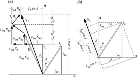
Fig. 3.1. Phasor diagram of an underexcited salient pole synchronous motor: (a) full phasor diagram; (b) auxiliary diagram for calculation of input power.

are obtained by solving the set of eqns (3.32). The rms armature current as a function of V₁, E_f, X_sd, X_sq, δ, and R₁ is

$\begin{matrix} I_{a} = \sqrt{I_{a d}^{2} + I_{a q}^{2}} = \frac{V_{1}}{X_{s d} X_{s q} + R_{1}^{2}} \\ × \sqrt{[(X_{s q} \cos δ - R_{1} \sin δ) - \frac{E_{f}}{V_{1}} X_{s q}]^{2} + [(R_{1} \cos δ + X_{s d} \sin δ) - \frac{E_{f}}{V_{1}} R_{1}]^{2}} \end{matrix} (3.35)$

The phasor diagram (Fig. 3.1) can also be used to find the input power [70], i.e.,

$P_{i n} = m_{1} V_{1} I_{a} \cos ϕ = m_{1} V_{1} (I_{a q} \cos δ - I_{a d} \sin δ) (3.36)$

Putting eqns (3.32) into eqn (3.36),

$\begin{matrix} P_{i n} = m_{1} [I_{a q} E_{f} + I_{a d} I_{a q} X_{s d} + I_{a q}^{2} R_{1} - I_{a d} I_{a q} X_{s q} + I_{a d}^{2} R_{1}] \\ = m_{1} [I_{a q} E_{f} + R_{1} I_{a}^{2} + I_{a d} I_{a q} (X_{s d} - X_{s q})] \end{matrix} (3.37)$

Because the armature core loss has been neglected, the electromagnetic power is the motor input power minus the armature winding loss $Δ P_{1 w} = m_{1} I_{a}^{2} R_{1} = m_{1} (I_{a d}^{2} + I_{a q}^{2}) R_{1}$ . Thus,

$\begin{matrix} P_{e l m} = P_{i n} - Δ P_{1 w} = m_{1} [I_{a q} E_{f} + I_{a d} I_{a q} (X_{s d} - X_{s q})] \\ = \frac{m_{1} [V_{1} (R_{1} \cos δ + X_{s d} \sin δ) - E_{f} R_{1})]}{{(X_{s d} X_{s q} + R_{1}^{2})}^{2}} \end{matrix} (3.38)$

Putting R₁ = 0, eqn (3.38) takes the following simple form,

$P_{e l m} = m_{1} [\frac{V_{1} E_{f}}{X_{s d}} \sin δ + \frac{V_{1}^{2}}{2} (\frac{1}{X_{s q}} - \frac{1}{X_{s d}})sin 2 δ] (3.39)$

Small PM LSMs have a rather high armature winding resistance R₁ that is comparable with X_sd and X_sq. That is why eqn (3.38), instead of (3.39), is recommended for calculating the performance of small, low-speed motors.

The electromagnetic thrust developed by a salient-pole LSM is

$\begin{matrix} F_{d x} = \frac{P_{e l m}}{v_{s}} & N \end{matrix} (3.40)$

Neglecting the armature winding resistance (R₁ = 0),

$F_{d x} = \frac{m_{1}}{v_{s}} [\frac{V_{1} E_{f}}{X_{s d}} \sin δ + \frac{V_{1}^{2}}{2} (\frac{1}{X_{s q}} - \frac{1}{X_{s d}})sin 2 δ] (3.41)$

Images

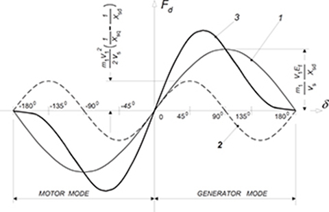
Fig. 3.2. Thrust-angle characteristics of a salient-pole synchronous machine with X_sd > X_sq. 1 — synchronous thrust F_dsyn developed by the machine, 2 — reluctance thrust F_drel, 3 — resultant thrust F_d.

In a salient-pole synchronous motor, the electromagnetic thrust has two components (Fig. 3.2)

$F_{d x} = F_{d x s y n} + F_{d x r e l} (3.42)$

where the first term,

$F_{d x s y n} = \frac{m_{1}}{v_{s}} \frac{V_{1} E_{f}}{X_{s d}} sin δ (3.43)$

is a function of both the input voltage V₁ and the excitation EMF E_f. The second term,

$F_{d x r e l} = \frac{m_{1} V_{1}^{2}}{2 v_{s}} (\frac{1}{X_{s q}} - \frac{1}{X_{s d}})sin 2 δ (3.44)$

depends only on the voltage V₁ and also exists in an unexcited machine (E_f = 0) provided that X_sd ≠ X_sq. The thrust F_dxsyn is called the synchronous thrust, and the thrust F_dxrel is called the reluctance thrust. The proportion between X_sd and X_sq strongly affects the shape of curves 2 and 3 in Fig. 3.2. For surface configurations of PMs, X_sd ≈ X_sq (if the magnetic saturation is neglected) and

$F_{d x} \approx F_{d x s y n} = \frac{m_{1}}{v_{s}} \frac{V_{1} E_{f}}{X_{s d}} sin δ (3.45)$

3.1.6 Minimization of d-axis Armature Current

For zero d-axis armature current, all current I_a = I_aq is torque producing. The d-axis armature current is zero (I_ad = 0) if the numerator of eqn (3.33) is zero, i.e.,

$V_{1} X_{s q} \cos δ - V_{1} R_{1} \sin δ - E_{f} X_{s q} = 0 (3.46)$

${(- V_{1} R_{1} \sin δ)}^{2} = {(E_{f} X_{s q} - V_{1} X_{s q} \cos δ)}^{2}$

After putting sin² δ = 1 − cos² δ, the following 2nd order linear equation is obtained,

$[{(V_{1} X_{s q})}^{2} + {(V_{1} R_{1})}^{2}] \cos^{2} δ - 2 V_{1} E_{f} X_{s q}^{2} cos δ + {(E_{f} X_{s q})}^{2} - {(V_{1} R_{1})}^{2} = 0 (3.47)$

$a x^{2} + b x + c = 0 (3.48)$

where x = cos δ, a = (V₁X_sq)² + (V₁R₁)², $b = - 2 V_{1} E_{f} X_{s q}^{2}$ , and c = (E_fX_sq)² − (V₁R₁)². Eqn (3.47) or eqn (3.48) has two roots:

$δ_{1} = arccos(x_{1}) = arccos (\frac{- b - \sqrt{Δ}}{2 a}) (3.49)$

$δ_{2} = arccos(x_{2}) = arccos (\frac{- b + \sqrt{Δ}}{2 a}) (3.50)$

where the discriminant of quadratic equation Δ = b² − 4ac. To obtain I_ad = 0, at least one root must be a real number. Sometimes both two roots are complex numbers. In this case, for motoring mode, most often the EMF E_f, is greater than the terminal voltage V₁. It means that the number of turns per phase must be reduced.

3.1.7 Thrust Ripple

The thrust ripple can be expressed as the rms thrust ripple $\sqrt{\sum F_{d x v}^{2}}$ weighted to the mean value of the thrust F_dx developed by the LSM, i.e.,

$f_{r} = \frac{1}{F_{d x}} \sqrt{\sum_{ν} F_{d x ν}^{2}} (3.51)$

The thrust ripple of an LSM consists of three components: (1) detent thrust (cogging thrust), i.e., interaction between the excitation flux and variable permeance of the armature core due to slot openings, (2) distortion of sinusoidal or trapezoidal distribution of the magnetic flux density in the air gap and, (3) phase current commutation and current ripple.

Case Study 3.1. Single-Sided PM LSM

A flat, short-armature, single-sided, three-phase LSM has a long reaction rail with surface configuration of PMs. High-energy sintered NdFeB PMs with the remanent magnetic flux density B_r = 1.1 T and coercive force H_c = 800 kA/m have been used. The armature magnetic circuit has been made of cold-rolled steel laminations Dk-66 (Table 2.3) The following design data are available: armature phase windings are Y-connected, number of pole pairs p = 4, pole pitch τ = 56 mm, air gap in the d-axis (mechanical clearance) g = 2.5 mm, air gap in the q-axis g_q = 6.5 mm, effective width of the armature core L_i = 84 mm, width of the core (back iron) of the reaction rail w = 84 mm, height of the armature core (yoke) h_1c = 20 mm, length of the overhang (one side) l_e = 90 mm, number of armature turns per phase N₁ = 560, number of parallel wires a_w = 2, number of armature slots s₁ = 24, width of the armature tooth c_t = 8.4 mm, height of the core (yoke) of the reaction rail h_2c = 12 mm, dimensions of the armature open rectangular slot: h₁₁ = 26.0 mm, h₁₂ = 2.0 mm, h₁₃ = 3.0 mm, h₁₄ = 1.0 mm, b₁₄ = 10.3 mm (see Fig. 2.17b), stacking coefficient of the armature core k_i = 0.96, conductivity of armature wire σ₂₀ = 57 × 10⁶ S/m at 20⁰C, diameter of armature wire d_wir = 1.02 mm, temperature of armature winding 75⁰C, height of the PM h_M = 4.0 mm, width of the PM w_M = 42.0 mm, length of the PM (in the direction of armature conductors) l_M = 84 mm, width of the pole shoe b_p = w_M = 42.0 mm, and friction coefficient for rollers at constant speed μ_v = 0.01.

The coil pitch w_c of the armature winding is equal to the pole pitch τ (full pitch winding).

The LSM is fed from a VVVF inverter, and the ratio of the line voltage to input frequency V_1L/f = 10. The PM LSM has been designed for continuous duty cycle to operate with the load angle δ corresponding to the maximum efficiency. The current density in the armature winding normally does not exceed j_a = 3.0 A/mm² (natural air cooling).

Calculate the steady-state performance characteristics for f = 20, 15, 10 and 5 Hz.

Solution

For V_1L/f = 10, the input line voltages are 200 V for 20 Hz, 150 V for 15 Hz, 100 V for 10 Hz, and 50 V for 5 Hz. Steady-state characteristics have been calculated using analytical equations given in Chapters 1, 2, and 3. The volume of the PM material per 2pτ is p×2h_M×w_M×l_M = 4×2×4×42×84 = 112, 896 mm³.

Given below are parameters independent of the frequency, voltage, and load angle δ:

number of slots per pole per phase q₁ = 1
winding factor k_w1 = 1.0
pole pitch measured in slots = 3
pole shoe to pole pitch ratio α_i = 0.75
coil pitch measured in slots = 3
coil pitch measured in millimeters w_c = 56 mm
armature slot pitch t₁ = 18.7 mm
width of the armature slot b₁₁ = b₁₂ = b₁₄ = 10.3 mm
number of conductors in each slot N_sl = 280
conductors cross section area to slot area (slot fill factor) k_fill = 0.2252
Carter’s coefficient k_C = 1.2
form factor of the excitation field k_f = 1.176
form factor of the d-axis armature reaction k_fd = 1.0
form factor of the q-axis armature reaction k_fd = 1.0
reaction factors k_ad = k_aq = 0.85
coefficient of leakage flux σ_l = 1.156
permeance of the air gap G_g = 0.1370 × 10⁻⁵ H
permeance of the PM G_M = 0.1213 × 10⁻⁵ H
permeance for leakage fluxes G_lM = 0.2144 × 10⁻⁶ H
magnetic flux corresponding to the remanent magnetic flux density Φ_r = 0.3881 × 10⁻² Wb
relative recoil magnetic permeability μ_rrec = 1.094
PM edge line current density J_M = 800, 000.00 A/m
mass of the armature core m_1c = 5.56 kg
mass of the armature teeth m_1t = 4.92 kg
mass of the armature conductors m_Cu = 15.55 kg
friction force F_r = 1.542 N

Then, resistances and reactances independent of magnetic saturation have been calculated,

armature winding resistance R₁ = 2.5643 Ω at 75°C
armature winding leakage reactance X₁ = 4.159 Ω at f = 20 Hz
armature winding leakage reactance X₁ = 1.0397 Ω at f = 5 Hz
armature reaction reactance X_ad = X_aq = 4.5293 Ω at f = 20 Hz
armature reaction reactance X_ad = X_aq = 1.1323 Ω at f = 5 Hz
specific slot leakage permeance λ_1s = 1.3918
specific leakage permeance of end connections λ_1e = 0.2192
specific tooth-top leakage permeance λ_1t = 0.1786
specific differential leakage permeance λ_1d = 0.21
coefficient of differential leakage τ_d1 = 0.0965

Note that for calculating X_ad of an LSM with surface PMs, the nonferromagnetic air gap is the gap between the ferromagnetic cores of the armature and reaction rail. The relative magnetic permeability of NdFeB PMs is very close to unity.

Steady-state performance characteristics have been calculated as functions of the load angle δ. The load angle of synchronous motors can be compared to the slip of induction motors, which is also a measure of how much the motor is loaded. Magnetic saturation due to main flux and leakage fluxes has been included. An LSM should operate with maximum efficiency. Maximum efficiency usually corresponds to the d-axis current I_ad ≈ 0. Table 3.2 shows fundamental steady-state performance characteristics for f = 20, 15, 10, and 5 Hz. In practice, the maximum efficiency corresponds to small values (close to zero) of the angle Ψ, i.e., the angle between the phasor of the armature current I_a and the q-axis, which means that the d-axis armature current I_ad for maximum efficiency is very small, or I_ad = 0 (Section 3.1.6 and Chapter 6).

Table 3.3 contains calculation results for maximum efficiency and two extreme frequencies f = 20 Hz and f = 5 Hz, including magnetic saturation. The magnetic flux density in armature teeth for maximum efficiency is well below the saturation magnetic flux density (over 2.1 T for Dk-69 laminations). This value is close to the saturation value for higher load angles δ ≥ 60⁰. Also, the armature current I_a and, consequently, line current density A_m and current density j_a increase with the load angle δ.

Table 3.2. Steady-state performance characteristics of a flat three-phase, four-pole LSM with surface PMs and τ = 56 mm

Images

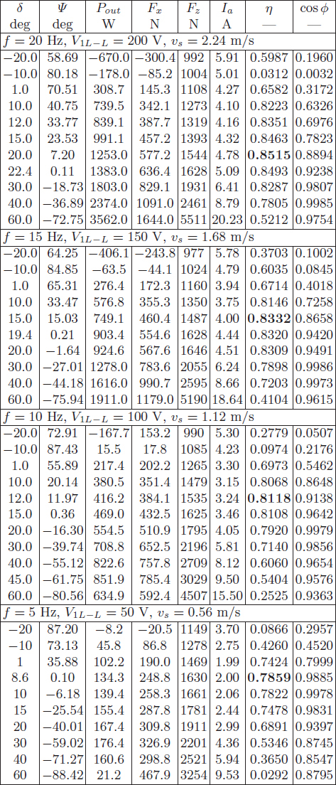
Table 3.3. Calculation results for maximum efficiency with magnetic saturation taken into account

Images

3.1.8 Magnetic Circuit

The equivalent magnetic circuit shown in Fig. 3.3 has been created on the basis of the following assumptions:

(a) Symmetry axis exists every 180° electrical degrees (one pole pitch).
(b) The magnetic flux density, magnetic field intensity and relative magnetic permeability in every point of each ferromagnetic portion of the magnetic circuit (PMs, cores, teeth) is constant.
(c) The air gap leakage flux is only between the heads of teeth.
(d) The magnetic flux of the armature (primary unit) penetrates only through the teeth and core (yoke).
(e) The equivalent reluctance of teeth per pole pitch is ℜ_t/Q₁, where ℜ_t is the reluctance of a single tooth and Q₁ is the number of teeth (slots) per pole.

Each portion of the magnetic circuit is replaced by equivalent reluctances:

reluctance of PM

$ℜ_{M} = \frac{h_{M}}{μ_{0} μ_{r r e c} w_{M} L_{M}} (3.52)$
reluctance of air gap

$ℜ_{g} = \frac{g k_{C}}{μ_{0} w_{M} l_{M}} = \frac{g k_{C}}{μ_{0} α_{i} τ L_{M}} (3.53)$
reluctance of a single tooth

$ℜ_{t} = \frac{h_{t}}{μ_{0} μ_{r t} c_{t} L_{i} k_{i}} (3.54)$
reluctance of the armature core (yoke) per pole pitch

$ℜ_{1 c} \approx \frac{τ + h_{1 c}}{μ_{0} μ_{r 1 c} h_{1 c} L_{i} k_{i}} (3.55)$
reluctance of a the reaction rail core (yoke) per pole pitch

$ℜ_{2 c} \approx \frac{τ + h_{2 c}}{μ_{0} μ_{r 2 c} h_{2 c} L_{M}} (3.56)$
reluctance for the PM leakage flux

$ℜ_{l M} = \frac{1}{G_{l M}} (3.57)$

in which

$\begin{matrix} G_{l M} \approx 2 μ_{0} (0.52 l_{M} + 0.26 w_{M} + 0.308 h_{M}) & if & h_{M} \leq x_{M} \end{matrix} (3.58)$

$\begin{matrix} G_{l M} \approx 2 μ_{0} (\frac{h_{M} l_{M}}{x_{M}} + 0.26 w_{M} + 0.308 h_{M}) & if & h_{M} > x_{M} \end{matrix} (3.59)$
reluctance for the air gap leakage flux

$ℜ_{l g} \approx \frac{1}{μ_{0}} \frac{5 + 4 g k_{C} / b_{14}}{5 g k_{C} / b_{14}} \frac{1}{L_{i}} (3.60)$

In the foregoing equations (3.52) to (3.60), μ_rrec is the relative recoil magnetic permeability of the PM, μ_rt is the relative magnetic permeability of the armature tooth, μ_r1c is the relative magnetic permeability of the armature core (yoke), μ_r2c is the relative magnetic permeability of the reaction rail (core), h_M is the height of the PM per pole, w_M is the width of the PM, and l_M is the length of the PM in the direction perpendicular to the plane of the traveling field, h_1c is the height of the armature core (yoke), h_2c is the height of the reaction rail core, b₁₄ is the armature slot opening, k_C is Carter’s coefficient, τ is the pole pitch, L_i is the effective length of the armature stack (in the direction perpendicular to laminations), and x_M is the distance between adjacent PMs. The magnetic flux Φ_f is excited by the MMF F_M = H_ch_M of PMs, the armature reaction MMF F_ad is given by eqn (3.19), Φ_f is the PM excitation flux (flux at no load), Φ_g is the air gap magnetic flux, and Φ is the magnetic flux linked with the primary winding (air gap flux Φ_g reduced by the air gap leakage flux Φ_lg, if included).

Images

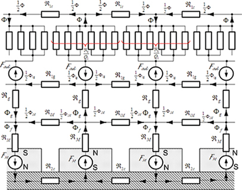
Fig. 3.3. Magnetic circuit of an LSM with surface PMs. Symbols are described in the text.

Reluctances for leakage fluxes ℜ_lM, according to eqns (3.57), (3.58), and (3.59), have been calculated by dividing the magnetic field into simple solids. The reluctance (3.58) is a parallel connection of the reluctances of two one-quarters of a cylinder (B.16), two half-cylinders (B.15), and four one-quarters of a sphere (B.21). The reluctance (3.59) is a parallel connection of the reluctances of two prisms (B.13), two half-cylinders (B.15), and four one-quarters of a sphere (B.21).

The following Kirchhoff’s equations can be written for the magnetic circuit presented in Fig. 3.3:

$2 Φ \frac{R_{t}}{Q_{1}} + \frac{1}{2} Φ ℜ_{1 c} - \frac{1}{2} Φ_{l g} ℜ_{l g} = - 2 F_{a d} (3.61)$

$Φ_{g} = Φ + Φ_{l g} (3.62)$

$Φ_{f} = Φ_{g} + Φ_{M} (3.63)$

$2 Φ_{f} ℜ_{M} + \frac{1}{2} Φ_{l M} ℜ_{l M} + \frac{1}{2} Φ_{f} ℜ_{2 c} = 2 F_{M} (3.64)$

$2(F_{M} - F_{a d}) = 2 Φ_{f} ℜ_{M} + 2 Φ_{g} ℜ_{g} + 2 Φ \frac{ℜ_{t}}{Q_{1}} + \frac{1}{2} Φ ℜ_{1 c} + \frac{1}{2} Φ_{f} ℜ_{2 c} (3.65)$

The solution to these equations gives magnetic fluxes in the following form,

magnetic flux excited by PMs

$Φ_{f} = \frac{2 (F_{M} - F_{a d} - 4 F_{a d} ℜ_{g} / ℜ_{l g}) A + 2 (F_{M} + F_{a d} ℜ_{l M} / ℜ_{l g})(2 / ℜ_{l M}) B}{A C + B D} (3.66)$
magnetic flux linked with the armature winding

$Φ = \frac{2 (F_{M} - F_{a d} - 4 F_{a d} ℜ_{g} / ℜ_{l g}) D - 2 (F_{M} + F_{a d} ℜ_{l M} / ℜ_{l g})(2 / ℜ_{l M}) C}{A C + B D} (3.67)$
air gap magnetic flux

$Φ_{g} = Φ A + \frac{4 F_{a d}}{ℜ_{l g}} (3.68)$

The leakage fluxes result from eqns (3.62) and (3.63), i.e.,

$Φ_{l g} = Φ_{g} - Φ (3.69)$

$Φ_{l M} = Φ_{f} - Φ_{g} (3.70)$

In the above eqns (3.66) to (3.68),

$A = 1 + \frac{1}{ℜ_{l g}} (2 \frac{ℜ_{t}}{Q_{1}} + \frac{1}{2} ℜ_{1 c}) (3.71)$

$B = 2 A ℜ_{g} + 2 \frac{ℜ_{t}}{Q_{1}} + \frac{1}{2} ℜ_{1 c} (3.72)$

$C = 2 ℜ_{P M} + \frac{1}{2} ℜ_{2 c} (3.73)$

$D = 1 + 4 \frac{ℜ_{M}}{ℜ_{l M}} + \frac{ℜ_{2 c}}{ℜ_{l M}} (3.74)$

The coefficient of PMs leakage flux

$σ_{l M} = 1 + \frac{Φ_{l M}}{Φ_{f}} (3.75)$

The coefficient of total leakage flux

$σ_{l} \approx 1 + \frac{Φ_{l M} + Φ_{l g}}{Φ_{f}} (3.76)$

If ℜ_lg → ∞ and ℜ_lM → ∞, then A → 1. It means that leakage fluxes Φ_lg → 0 and Φ_lM → 0. Thus, the magnetic flux

$Φ_{f} = Φ_{g} = Φ = \frac{2 (F_{M} - F_{a d})}{2 (ℜ_{M} + ℜ_{g} + \frac{ℜ_{t}}{Q_{1}}) + 0.5 (ℜ_{1 c} + ℜ_{2 c})} (3.77)$

3.1.9 Direct Calculation of Thrust

The thrust of a PM LSM can be calculated directly on the basis of the electromagnetic field distribution [152]. Fig. 3.4 shows a single-sided PM LSM in the Cartesian coordinate system. The problem can be simplified to a two-dimensional (2D) field distribution where currents (y direction) in the armature winding are perpendicular to the laminations, and magnetic flux density has only two components, i.e., tangential component B_x and normal component B_z.

The 2D electromagnetic field distribution will be found on the basis of the following assumptions:

(a) The armature core is an isotropic and slotless cube with its magnetic permeability tending to infinity and electric conductivity tending to zero.
(b) The armature winding is represented by an infinitely thin current sheet distributed uniformly at the active surface of the armature core.
(c) The armature currents flow only in the direction perpendicular to the xz plane, i.e., in the y direction.
(d) The width of the PM is b_p < τ.

Fig. 3.4. Model of a single-sided LSM with surface configuration of PMs for 2D electromagnetic field analysis.
(e) Isotropic PMs are magnetized in the normal direction (z coordinate) and have zero electric conductivity.
(f) Each PM is represented by an equivalent coil embracing the PM and carrying a fictitious surface current that produces an equivalent magnetic flux.
(g) The magnetic permeability of the space between PMs is equal to that of PMs.
(h) The core of the reaction rail is an isotropic cube with its magnetic permeability tending to infinity and electric conductivity tending to zero.

Simplifications given by assumptions (a) and (b) can be corrected by replacing the air gap g between the armature core and PMs by an equivalent air gap g = k_Cg, where k_C is Carter’s coefficient. The time-space distribution of the armature line current density for the fundamental space harmonic can be obtained by taking the first derivative of the primary MMF distribution with respect to the x coordinate. According to eqns (3.7) and (3.8),

$a (x, t) = \frac{d F (x, t)}{d x} = - \frac{m_{1} \sqrt{2}}{p τ} N_{1} I_{a} k_{w 1} cos(ω t - β x) (3.78)$

$a (x, t) = - R e [A_{m} e^{j ω t - β x}] = - R e [A_{m} e^{j ω t} e^{- j β x}] (3.79)$

where the peak value of the line current density

$A_{m} = \frac{m_{1} \sqrt{2} N_{1} k_{w 1} I_{a}}{p τ} (3.80)$

and the constant

$β = \frac{π}{τ} (3.81)$

The line current density (3.80) obtained as dF(x, t)/dx has in numerator the effective number of turns N₁k_w1, instead of the number of turns N₁ — see eqn (3.9). Eqn 3.9) is according to the definition of the line current density.

The space distribution of the armature line current density is simply

$a (x) = - Re [A_{m} e^{- j β x}] = - A_{m} \cos β x (3.82)$

According to assumption (f) and for 2D problem, the equivalent edge line current density [152] representing a PM is the same as H_c for the linear demagnetization curve, i.e.,

$\begin{matrix} J_{M} = \frac{B_{r}}{μ_{0} μ_{r r e c}} & A / m \end{matrix} (3.83)$

where B_r is the remanent magnetic flux density, and μ_rrec is the relative recoil magnetic permeability of a PM (Chapter 2 and Appendix A). If, say, B_r = 1.1 T and μ_rrec = 1.05, the equivalent edge line current density J_M ≈ 0.834×10⁶ A/m.

The PM magnetic flux density equal to the remanent flux density B_r is constant over the whole width b_p = α_iτ of the PM and takes its sign according to the polarity of PMs. Such a periodical function $b (x) = \sum_{v = 1}^{\infty} b_{v} \sin (v π x / τ)$ can be resolved into Fourier series the coefficient b_ν of which, for the fundamental harmonic

$\frac{2}{τ} \int_{0.5 (τ - b_{p})}^{05 (τ + b_{p})} B_{r} sin(β x) d x = B_{r} \frac{4}{π} sin \frac{α_{i} π}{2} = B_{r} k_{f} (3.84)$

is equal to the product of B_r times the form factor of the excitation field according to eqn (3.10). Thus, the equivalent current density distribution representing the PM for ν = 1 is

$j_{M} (x) = k_{f} \frac{B_{r}}{μ_{0} μ_{r}} \sin β x = k_{f} J_{M} sin(β x) (3.85)$

Assumption (g) can be partially justified due to the fact that the relative magnetic permeability of the NdFeB PM is usually 1.0 to 1.1, i.e., close to the relative magnetic permeability of free space.

The 2D electromagnetic field distribution excited by the armature winding in both regions I and II (Fig. 3.4) can be described by Laplace’s equation

$\frac{\partial^{2} A}{\partial x^{2}} + \frac{\partial^{2} A}{\partial z^{2}} = 0 (3.86)$

where A is the magnetic vector potential defined as B = curlA (B = ∇A).

Using the method of separation of variables, the solution to eqn (3.86) for the fundamental space harmonic can have the following form:

$A_{y} (x, z, t) = e^{j (ω t - β x)} (A e^{- β z} + B e^{β z}) (3.87)$

According to eqn (3.82), the space distribution of the primary line current density is according to cosinusoidal law. Hence, the line current density given by eqn (3.87) can be expressed as a real number, i.e.,

$A_{y} (x, z) = \cos (β x)(A e^{- β z} + B e^{β z}) (3.88)$

According to assumption (c), the magnetic vector potential can only have one component A_y in the y direction so that, in the Cartesian coordinate system,

$\begin{matrix} B_{x} = - \frac{\partial A_{y}}{\partial z} & B_{z} = - \frac{\partial A_{y}}{\partial x} \end{matrix} (3.89)$

The components of the magnetic flux density in region I and region II are

$B_{x} (x, z) = - \frac{\partial A_{y} (x, z)}{\partial z} = β \cos (β x)(A e^{- β z} - B e^{β z}) (3.90)$

$B_{z} (x, z) = \frac{\partial A_{y} (x, z)}{\partial x} = - β \sin (β x)(A e^{- β z} + B e^{β z}) (3.91)$

On the basis of assumption (a), the magnetic permeability of the primary stack tends to infinity. Thus, at z = 0,

$\frac{B_{x I} (x, z = 0)}{μ_{0}} = a (x)$

or, on the basis of eqn (3.82),

$β (A_{I} - B_{I}) = - μ_{0} A_{m} (3.92)$

where the amplitude of the line current density A_m is according to eqn (3.80).

At z = g,

$\begin{matrix} \frac{B_{x I} (x, z = g)}{μ_{0}} = \frac{B_{x I I} (x, z = g)}{μ_{0} μ_{r r e c}} & and & B_{z I} (x, z = g) = B_{z I I} (x, z = g) \end{matrix}$

$μ_{r r e c} (A_{I} e^{- β g} - B_{I} e^{β g}) = A_{I I} e^{- β g} - B_{I I} e^{β g} (3.93)$

$A_{I} e^{- β g} + B_{I} e^{β g} = A_{I I} e^{- β g} + B_{I I} e^{β g} (3.94)$

At z = g + h_M,

$B_{x} (x, z = g + h_{M}) = 0$

$A_{I I} e^{- β (g + h_{M})} - B_{I I} e^{β (g + h_{M})} = 0 (3.95)$

The foregoing boundary conditions allow for finding all constants A_I, A_II, B_I, and B_II (four equations). For example, the constants A_II and B_II are

$\begin{matrix} A_{I I} = C' e^{β (g + h_{M})} & B_{I I} = C' e^{- β (g + h_{M})} \end{matrix}$

where

$C' = \frac{1}{μ_{r r e l} cosh(β h_{M})sinh(β g) + sinh(β h_{M})cosh(β g}) \frac{μ_{0} μ_{r r e l}}{2 β} A_{m}$

Putting the constants A_II and B_II into eqns (3.91), the space distribution of the first harmonic of the normal component of the armature magnetic flux density is

$B_{z I I} (x, z) = - 2 β C' \sin (β x)cosh [β (g + h_{M} - z)] (3.96)$

The thrust for the fundamental harmonic can be found on the basis of the Lorentz equation. The force increment acting on an edge with the coordinate x = b_p/2 and line current density J_M is dF_dx = B_zII(x = 0.5b_p, z)J_ML_idz. For 2 × 2p edges and neglecting the “–” sign

$\begin{matrix} F_{d x} = 8 p L_{i} J_{M} β C' \int_{g}^{g + h_{M}} \sin α_{i} \frac{π}{2} \cosh [β (g + h_{M} - z)] d z \\ \int_{g}^{g + h_{M}} \cosh [β (h_{M} + g - z)] d z = \frac{1}{β} sinh(β h_{M}) = \frac{τ}{π} sinh(β h_{M}) \end{matrix} (3.97)$

Finally,

$F_{d x} = \frac{4}{π} p τ L_{i} B_{r} A_{m} sin(\frac{α_{i} π}{2}) \frac{tanh(β h_{M})}{μ_{r r e l} sinh(β g) + \tanh (β h_{M})cosh(β g}) (3.98)$

The above eqn (3.98) has been derived and verified by H. Mosebach [152] and then developed further for armature line current waveforms other than sinusoidal [153].

3.2 Motors with Superconducting Excitation Coils

The model of a coreless LSM with SC electromagnets is shown in Fig. 3.5 [14, 62, 124, 190]. The following assumptions have been made to find the 2D distribution of magnetic and electric field components:

(a) The armature winding is represented by an infinitely long (x direction) and infinitely thin (z direction) current sheet that is distributed uniformly at z = g (xy surface).
(b) The distribution of electromagnetic field in the x direction is periodical with the period equal to 2τ.
(c) The armature currents flow only in the direction perpendicular to the xz plane, i.e., in the y direction.
(d) The air-cored excitation winding is represented by an infinitely thin current sheet distributed uniformly at the z = 0 of the xy surface.
(e) The electromagnetic field does not change in the y direction.
(f) End effects due to the finite length of windings (x direction) are neglected.
(g) Only the fundamental space harmonic ν = 1 of the field distribution in the x direction is taken into account.

Images

Fig. 3.5. Model of an air-cored LSM with SC excitation system for the electromagnetic field analysis: (a) winding layout, (b) armature and field excitation current sheets.

The armature winding can be represented by the following space-time distribution of the line current density (current sheet) expressed as a complex number

$a(x, t) = A_{m} e^{j (ω t - β x)} (3.99)$

and the field excitation winding can be described by the following space-time distribution of the complex line current density

$a_{f} (x, t) = A_{m f} e^{j (ω t - β x - ε)} (3.100)$

where the peak values of line current densities are

for the armature winding — see eqn (3.80)

$A_{m} = \frac{m_{1} \sqrt{2} N_{1} k_{w 1} I_{a}}{p τ} = \frac{2 m_{1} \sqrt{2} N_{1 p} k_{w 1} I_{a}}{τ} (3.101)$
for the field excitation winding (d.c. current excitation)

$A_{m f} = \frac{2 N_{f} k_{w f} I_{f}}{p τ} = \frac{4 N_{f p} k_{w f} I_{f}}{τ} (3.102)$

The number of series armature turns per phase is N₁ = 2pN_1p where N_1p is the number of armature series turns per phase per pole, and the number of field series turns N_f = 2pN_fp where N_fp is the number of field turns per pole.

The so-called force angle = 90⁰ ∓ Ψ is the angle between phasors of the excitation flux Φ_f in the d-axis and the armature current I_a.

The 2D distribution of the magnetic vector potential of the field excitation winding is described by the Laplace’s equation

$\frac{\partial^{2} A_{f y}}{\partial x^{2}} + \frac{\partial^{2} A_{f y}}{\partial z^{2}} = 0 (3.103)$

The general solution to eqn (3.103) for 0

$A_{f y} (x, z) = C_{f} e^{j (ω t - β x - ε)} e^{- β z} (3.104)$

On the basis of the definition of the magnetic vector potential, there are only two components of the magnetic flux density of the field excitation winding, i.e.,

$\begin{matrix} B_{f x} = - \frac{\partial A_{f y}}{\partial z} = β A_{f y} & B_{f z} = \frac{\partial A_{f y}}{\partial x} = - j β A_{f y} \end{matrix} (3.105)$

According to Ampère’s circuital law applied to the field excitation current sheet (z = 0),

$2 \int H_{f x} (x, z = 0) d x = \int a(x, t) d x$

and using the first eqn (3.105),

$H_{f x} (x, z = 0) = \frac{B_{f x} (x, z = 0)}{μ_{0}} = - \frac{1}{μ_{0}} \frac{\partial A_{f y} (x, z = 0)}{\partial z} = \frac{β}{μ_{0}} A_{f y} (x, z = 0)$

The constant C_f in eqn (3.104) is

$C_{f} = \frac{μ_{0} A_{m f}}{2 β}$

and

$A_{f y} (x, z) = \frac{μ_{0}}{2 β} A_{m f} e^{j (ω t - β x - ε)} e^{- β z} (3.106)$

The components B_fx and B_fz can be found on the basis of eqns (3.105) and (3.106).

The magnetic vector potential of the armature winding has a similar form as eqn (3.106), i.e.,

$A_{y} (x, z) = \frac{μ_{0}}{2 β} A_{m} e^{j (ω t - β x)} e^{- β (g - z)} (3.107)$

The forces in the x and z direction per unit area can be found on the basis of the Lorentz equation, i.e.,

tangential force

$\begin{matrix} f_{d x} = \frac{1}{2} R e [a(x, t) B_{f z}^{*}] = - \frac{1}{4} μ_{0} A_{m} A_{m f} e^{- β g} \sin ε & N / m^{2} \end{matrix} (3.108)$
normal force

$\begin{matrix} f_{d z} = - \frac{1}{2} R e [a(x, t) B_{f x}^{*}] = - \frac{1}{4} μ_{0} A_{m} A_{m f} e^{- β g} \cos ε & N / m^{2} \end{matrix} (3.109)$

Multiplying by the area 2pτ of the SC electromagnet,

the electromagnetic thrust

$F_{d x} = - F_{m a x} \sin ε (3.110)$
the normal repulsive force

$F_{d z} = - F_{m a x} \cos ε (3.111)$

where the peak force

$F_{m a x} = 4 μ_{0} m_{1} p \sqrt{2} N_{1 p} k_{w 1} N_{f p} k_{w f} \frac{L_{i}}{τ} I_{a} I_{f} e^{- β g} (3.112)$

Case Study 3.2. Single-Sided Air-Cored LSM

Given are the following design data of a single-sided air-cored LSM with SC excitation winding (Figs 1.17 and 3.5): m₁ = 3, p = 2, N_fpk_wfI_f = 700 × 10³ A, k_w1 = 1.0, I_a = 1000 A, g = 0.1 m, τ = 1.35 m, and L_i = 1.07 m. Find:

(a) The maximum force as a function of the number of armature turns 2 ≤ N_1p ≤ 20
(b) The electromagnetic thrust F_dx and normal force F_dz as functions of the force angle ∈.

Images

Fig. 3.6. Electromagnetic thrust F_dx and normal force F_dz as functions of the force angle for typical parameters of an air-cored LSM.

Solution

The maximum force for N_1p = 2 is

$\begin{matrix} F_{m a x} = 4 \times 0.4 π \times 10^{- 6} \times 3 \times 2 \times \sqrt{2} \times 2 \times 1.0 \times 700 \times 10^{3} \times 1000.0 \\ \times \frac{1.07}{1.35} e^{- 0.1 π / 135} = 37, 501.4 N \approx 37 .5kN \end{matrix}$

For N_1p = 5, F_max = 93.75 kN; for N_1p = 10, F_max = 187.5 kN; for N_1p = 15, F_max = 281.25 kN; and for N_1p = 20, F_max = 375.0 kN. The “−” sign has been neglected.

The forces F_dx = F_max sin ∈ and F_dz = F_max cos ∈ as functions of are plotted in Fig. 3.6.

3.3 Double-Sided LSM with Inner Moving Coil

The analysis of electromagnetic field in a double-sided PM LSM (Fig. 2.24) will be performed on the basis of the following assumptions:

(a) All regions are extended to infinity in the ±x direction.
(b) Magnetic permeability of ferromagnetic core (return path for magnetic flux) tends to infinity.
(c) Isotropic PMs are magnetized in the normal direction (z coordinate) and have zero electric conductivity.
(d) PMs are represented by an equivalent line current density varying periodically with the period of 2τ/ν, where ν = 1, 3, 5, ….
(e) The model is linear.
(f) Armature reaction is negligible.

Images

Fig. 3.7. A layer model of a double-sided PM LSM with inner moving coil (I_a = 0).

A layer model is shown in Fig. 3.7. The armature current is assumed to be zero (I_a = 0), i.e., there is no armature reaction. Thus, the electromagnetic field in the air is described by Laplace’s equation, and in PMs by Poisson equation [77, 228], i.e.,

for −0.5g ≤ z ≤ 0.5g

$\frac{\partial^{2} A_{I} (x, z)}{\partial x^{2}} + \frac{\partial^{2} A_{I} (x, z)}{\partial z^{2}} = 0 (3.113)$
for −0.5g + h_m ≤ z ≤ 0.5g + h_M

$\frac{\partial^{2} A_{I I} (x, z)}{\partial x^{2}} + \frac{\partial^{2} A_{I I} (x, z)}{\partial z^{2}} = - μ_{r e c} j_{M} (x) (3.114)$

where μ_rec = μ₀μ_rrec is the recoil permeability of PM; A_I and A_II are magnetic vector potentials in the air and PMs, respectively; and j_M(x) is the PM equivalent line current density, which can be written in the following scalar form:

$j_{M} (x) = \sum_{ν = 1, 3, \dots}^{\infty} J_{M} \frac{4}{ν π} sin(ν α_{i} \frac{π}{2})sin(β_{ν} x) (3.115)$

where ν = 1, 3, 5, … are higher space harmonics, τ is pole pitch, J_M is given by eqn (3.83), and

$β_{ν} = ν β = ν \frac{π}{τ} (3.116)$

See also eqns (3.81) and (3.85) in which ν = 1. Using the method of variable separation, general solutions to eqns (3.113) and (3.114) are

$A_{I} = \sum_{ν = 1, 3, \dots}^{\infty} (C_{1} e^{- β_{ν} z} + C_{2} e^{β_{ν} z})sin(β_{ν} x) (3.117)$

$A_{I I} = \sum_{ν = 1, 3, \dots}^{\infty} [C_{3} e^{- β_{ν} z} + C_{4} e^{β_{ν} z} + \frac{4 B_{r^{T}}}{ν^{2} π^{2}} sin(β_{ν} x)] sin(β_{ν} x) (3.118)$

On the basis of assumption (b), the following boundary condition can be written,

$\begin{matrix} \begin{matrix} z = 0 & H_{I} = 0 \end{matrix} \\ \begin{matrix} z = ± 0.5 g & H_{x I} = H_{x I I} & and & B_{z I} = B_{z I I} \end{matrix} \\ \begin{matrix} z = ±(0.5 g + h_{M}) & H_{x I I} = 0 \end{matrix} \end{matrix} (3.119)$

From the above boundary conditions (3.119), constants C₁, C₂, C₃, and C₄ can be found, i.e.,

$\begin{matrix} C_{1} = C_{2} e^{- β_{ν} g} \\ C_{2} = \frac{4 B_{r^{T}}}{ν^{2} π^{2}} sin(β_{ν} x) \end{matrix} (3.120)$

$× \frac{1}{(e^{- β_{ν} g} + 1) + \frac{1}{μ_{0} (e^{2 β_{ν} h_{M}} - 1)} [μ_{r e c} (- e^{- β_{ν} g} + 1)] (e^{2 β_{ν} h_{M}} - 1)} (3.121)$

$C_{3} = C_{4} e^{2 β_{ν} h_{M}} (3.122)$

$C_{4} = μ_{r e c} (- e^{- β_{ν} g} + 1) \frac{1}{e^{2 β_{ν} h_{M}} - 1} C_{2} (3.123)$

The magnetic flux density components can be found from the definition of the magnetic vector potential B = ∇ × A. For example, the normal component of the magnetic flux density in the middle of the air gap is

$\begin{matrix} B_{z I} (x) = - \frac{\partial A}{\partial x} \\ = - \sum_{ν = 1, 3, \dots}^{\infty} β_{ν} (C_{1} e^{0.5 β_{ν} g} + C_{2} e^{- 0.5 β_{ν} g})cos(β_{ν} x) \end{matrix} (3.124)$

Eqn (3.124) does not include the armature field (I_a = 0), but only the PM excitation field.

3.4 Variable Reluctance Motors

The variable reluctance LSM, called simply the linear reluctance motor (LRM), does not have any excitation system, so the EMF E_f = 0. The thrust is expressed by eqn (3.44) and is proportional to the input voltage squared $V_{1}^{2}$ , the difference X_sd−X_sq between the d- and q-axis synchronous reactances and sin(2δ) where δ is the load angle (between the terminal voltage V₁ and the q-axis). Including the stator winding resistance R₁, the thrust is

$\begin{matrix} F_{d x r e l} = \frac{P_{e l m}}{v_{s}} = \frac{m_{1} V_{1}^{2}}{2 v_{s}} \frac{X_{s d} - X_{s q}}{{(X_{s d} X_{s q} + R_{1}^{2})}^{2}} [(X_{s d} X_{s q} - R_{1}^{2})sin 2 δ \\ + R_{1} (X_{s d} + X_{s q})cos 2 δ - R_{1} (X_{s d} - X_{s q})] \end{matrix} (3.125)$

where P_elm is according to eqn (3.38) for E_f = 0.

For the same load, the input current of a reluctance LSM is higher than that of a PM LSM since the EMF induced in the armature winding by the field excitation system is zero — eqns (3.33) and (3.34). Correspondingly, it affects efficiency because of higher power loss dissipated in the armature winding. The thrust can be increased by magnifying the ratio X_sd/X_sq. However, this in turn involves a heavier magnetizing current, resulting in further increase in the input current due to a high reluctance of the magnetic circuit in the q-axis.

3.5 Switched Reluctance Motors

The inductance of a linear switched reluctance motor (Fig. 1.21) can be approximated by the following function (see also eqn 5.9):

$\begin{matrix} L (x) = \frac{1}{2} (L_{m a x} + L_{m i n}) - \frac{1}{2} (L_{m a x} - L_{m i n})cos(\frac{π}{τ} x) \\ = L_{0} - \frac{1}{2} (k_{L} - 1) L_{m a x} \cos \frac{π}{τ} x \end{matrix} (3.126)$

where

$L_{0} = \frac{1}{2} (L_{m a x} + L_{m i n}) (3.127)$

$k_{L} = \frac{L_{m a x}}{L_{m i n}} (3.128)$

L_max is the maximum inductance (armature and platen poles are aligned), and L_min is the minimum inductance (complete misalignment of armature and platen poles).

If the magnetic saturation is negligible (magnetization characteristic is linear), the electromagnetic thrust (in the x-direction) according to eqns (1.11) and (1.13) is

$F_{d x} = \frac{d W}{d x} = \frac{1}{2} I_{a}^{2} \frac{d L (x)}{d x} = F_{m a x} I_{a}^{2} sin(\frac{π}{τ} x) (3.129)$

where the maximum force at I_a = 1 A

$F_{m a x} = \frac{1}{4} \frac{π}{τ} (k_{L} - 1) L_{m i n} (3.130)$

The electromagnetic thrust of a linear switched reluctance motor is directly proportional to the armature current squared $I_{a}^{2}$ and the ratio k_L of maximum to minimum inductance, and it is inversely proportional to the pole pitch τ. Eqns (3.129) and (3.130) do not take into account the current waveform shape and current turn-on and turn-off instants.

The thrust changes direction at the aligned position of the armature and the reaction rail poles. If the reaction rail continues past the aligned position, the attractive force between the armature and reaction rail poles produces retarding (braking) force. An accurate current turn-off instant provides elimination of braking force.

Sensitivity analysis of the effect of geometrical parameters on the performance of a linear switched reluctance motor, especially on the thrust profile, is given, e.g., in [9].

Examples

Example 3.1

A single-sided 6-pole, Y-connected PM LSM with surface configuration of PMs is fed with 230 V line-to-line voltage at 50 Hz. The number of turns per phase is N₁ = 180, winding factor k_w1 = 1, pole pitch τ = 48 mm, armature winding resistance per phase R₁ = 1.614 Ω, armature winding leakage reactance per phase X₁ = 2.246 Ω, d-axis armature reaction reactance X_ad = 2.710 Ω, q-axis armature reaction reactance X_aq = 2.515 Ω, magnetic flux density in the armature teeth is the same as that in core (yoke), i.e., B_1t = B_1c = 1.468 T, mass of armature teeth m_1t = 2.973 kg, mass of armature core (yoke) m_1c = 2.473 kg, the magnetic flux of PMs linked with the armature winding under load is Φ = 2.124×10⁻³ Wb, specific armature core losses δp_1/50 = 1.07 W/kg, windage losses ΔP_wind = 10 W, mechanical losses in linear bearings ΔP_m = 80 W, and losses in PMs ΔP_{P M} = 24.6 W. The armature coils are wound with two (a_w = 2) parallel copper conductors AWG20 (0.812 mm diameter). Find the parameters at load angle δ = 12° and steady-state performance characteristics.

Solution

The phase voltage is $V_{1} = 230 / \sqrt{3} = 132.8 V$ . The EMF per phase induced in the armature winding

$E_{f} = π \sqrt{2} \times 50 \times 180 \times 1.0 \times 2.124 \times 10^{- 3} = 84.95 V$

Synchronous reactances

$\begin{matrix} X_{s d} = 2.246 + 2.710 = 4.956 Ω \\ X_{s q} = 2.246 + 2.515 = 4.761 Ω \end{matrix}$

For δ = 12°, the d- and q-axis armature currents according to eqns (3.33) and (3.34) are

$\begin{matrix} I_{a d} = \frac{132.8 [4.761 \times \cos (12^{\circ}) - 1.614 \times \sin (12^{\circ})] - 84.95 \times 4.761}{4.956 \times 4.761 + {1.614}^{2}} = 6.466 A \\ I_{a q} = \frac{132.8 [1.614 \times \cos (12^{\circ}) + 4.956 \times sin(12^{\circ})] - 84.95 \times 1.614}{4.956 \times 4.761 + {1.614}^{2}} = 7.99 A \end{matrix}$

The total armature current

$I_{a} = \sqrt{6466^{2} + 799^{2}} = 10.8 A$

The angle between the armature current and the q-axis

$ψ = arcsin (\frac{6.466}{10.8}) = {38.98}^{\circ} = 0.68 rad$

Armature winding losses

$Δ P_{1 w} = 3 \times {10.8}^{2} \times 1.614 = 511.6 W$

Losses in armature teeth and core (yoke) according to eqn (2.3),

$Δ P_{F e} = 1.07 \times {(\frac{50}{50})}^{4 / 3} (1.8 \times {1.468}^{2} \times 2.973 + 3.0 \times {1.468}^{2} \times 2.473) = 29.4 W$

where k_adt = 1.8 and k_adc = 3.0. Total losses

$Δ P = 511.6 + 29.4 + 80 + 10 + 24.6 = 655.6 W$

Electromagnetic power calculated on the basis of eqn (3.38)

$P_{e l m} = 3 [10.8 \cos (12^{\circ}) \times 84.95 + 6.466 \times 7.99 (4.956 - 4.761)] = 2066.4 W$

Input power

$P_{i n} = P_{e l m} + Δ P_{1 w} + Δ P_{F e} = 2066.4 + 511.6 + 29.4 = 2607.5 W$

Output power

$P_{o u t} = P_{i n} - Δ P = 2607.5 - 655.6 = 1951.8 W$

Input apparent power

$S_{i n} = 3 \times 132.8 \times 10.8 = 4095.0 VA$

Power factor cos φ

$\begin{matrix} \cos ϕ = \frac{P_{i n}}{S_{i n}} = \frac{2607.5}{4095.0} = 0.637; & ϕ = arccos ϕ = {50.45}^{\circ} \end{matrix}$

Phase voltage across input terminals of the armature winding calculated according to eqn (3.32),

$\begin{matrix} V_{1} = \frac{1}{\cos ϕ} (E_{f} + I_{a d} X_{s d} + I_{a q} R_{1}) \\ = \frac{1}{0.637} (84.95 + 6.466 \times 4.956 + 7.99 \times 1.614) = 132.8 V \end{matrix}$

Linear synchronous speed

$v_{s} = 2 \times 50 \times 0.048 = 4.8 m / s$

Electromagnetic thrust (force in the x-direction)

$F_{d x} = \frac{2066.4}{4.8} = 430.5 N$

Output power calculated on the basis of electromagnetic power

$P_{o u t} = P_{e l m} - Δ P_{m} - Δ P_{w i n d} - Δ P_{P M} 2066.4 - 80.0 - 10.0 - 24.6 = 1951.8 W$

Useful thrust

$F_{x} = \frac{1951.8}{4.8} = 406.6 N$

Efficiency

$η = \frac{1951.8}{2607.5} = 0.749$

Images

Fig. 3.8. Output power P_out, electromagnetic power P_elm, input power P_in, and total losses ΔP plotted against armature current I_a.

Images

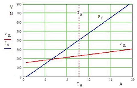
Fig. 3.9. Line voltage V_1L and useful thrust F_x plotted against armature current I_a.

Current density in the armature winding

$j_{a} = \frac{10.8}{2 \times (π \times {0.000812}^{2} / 4} = 9.93 \times 10^{6} A / m^{2}$

Line current density (peak value)

$A_{m} = \frac{3 \sqrt{2} 180 \times 10.8}{3 \times 0.048} = 54514 A / m$

Images

Fig. 3.10. Efficiency η and power factor cos φ plotted against armature current I_a.

EMF constant

$k_{E} = \frac{E_{f}}{v_{s}} = \frac{84.95}{4.8} = 17.697 Vs / m$

Force constant

$k_{F} = \frac{F_{d x}}{I_{a}} = \frac{430.5}{10.8} = 41.881 N / A$

Performance characteristics as functions of the armature currents are plotted in Figs 3.8, 3.9, and 3.10.

Example 3.2

A single-sided PM LSM has the following resistances and reactances: R₁ = 2.8 Ω, X₁ = 3.8 Ω, X_ad = 4.76 Ω, X_aq = 4.57 Ω. At frequency f = 50 Hz and phase voltage V₁ = 220 V, the EMF per phase is E_f = 200 V. The armature windings are Y-connected. The pole pitch is τ = 40 mm. Find the armature current I_a, electromagnetic power P_elm, electromagnetic thrust F_dx, and primary winding losses at zero d-axis armature current.

Solution

Synchronous reactances in the d- and q-axis

$\begin{matrix} X_{s d} = 3.8 + 4.76 = 8.56 Ω; & X_{s q} = 3.8 + 4.57 = 8.37 Ω \end{matrix}$

The discriminant of the quadratic equation (3.48) is

$Δ = b^{2} - 4 a c = {(- 6.165 \times 10^{6})}^{2} - 4 \times 3.77 \times 10^{6} \times 2.423 \times 10^{6} = 1.212 \times 10^{6} V^{6} {/A}^{2}$

where

$\begin{matrix} a = {(V_{1} X_{s q})}^{2} + {(V_{1} R_{1})}^{2} = {(220 \times 8.37)}^{2} + {(220 \times 2.8)}^{2} = 3.77 \times 10^{6} V^{3} /A \\ b = - 2 V_{1} E_{f} X_{s q}^{2} = - 2 \times 220 \times 200 \times {8.37}^{2} = - 6.165 \times 10^{6} V^{3} /A \\ c = {(E_{f} X_{s q})}^{2} - {(V_{1} R_{1})}^{2} = {(200 \times 8.37)}^{2} - {(220 \times 2.8)}^{2} = 2.423 \times 10^{6} V^{3} /A \end{matrix}$

Roots of the second-order equation (3.48)

$\begin{matrix} x_{1} = \frac{6.165 \times 10^{6} - \sqrt{1212 \times 10^{6}}}{2 \times 3.77 \times 10^{6}} = 0.657 \\ x_{2} = \frac{6.165 \times 10^{6} + \sqrt{1212 \times 10^{6}}}{2 \times 3.77 \times 10^{6}} = 0.978 \\ \begin{matrix} δ_{1} = arccos(x_{1}) = {48.94}^{\circ} & δ_{2} = arccos (x_{2}) = {11.95}^{\circ} \circ \end{matrix} \end{matrix}$

For δ₂ = 11.95°, the armature currents according to eqns (3.33) and (3.34) are

$\begin{matrix} I_{a d} = \frac{220 [8.37 \times \cos ({11.95}^{\circ}) - 2.8 \times \sin ({11.95}^{\circ})] - 200 \times 8.37}{8.56 \times 8.37 + {2.8}^{2}} = 0 A \\ I_{a q} = \frac{220 [2.8 \times \cos ({11.95}^{\circ} \circ) + 8.56 \times a({11.95}^{\circ})] - 200 \times 2.8}{8.56 \times 8.37 + {2.8}^{2}} = 5.44 A \end{matrix}$

The total armature current is torque producing, i.e.,

$I_{a} = \sqrt{0^{2} + 544^{2}} = 5.44 A$

The angle between the primary current and q-axis must be zero, i.e.,

$ψ = arcsin (\frac{I_{a d}}{I_{a}}) = 0^{o}$

Electromagnetic power at I_ad = 0 is calculated on the basis of eqn (3.38):

$P_{e l m} = 3 [5.44 \times 200 + 0 \times 5.44 (8.56 - 8.37)] = 3265 W$

Linear synchronous speed

$v_{s} = 2 \times 50 \times 0.04 = 4.0 m / s$

Electromagnetic force at I_ad = 0

$F_{d x} = \frac{3265}{4.0} = 816.3 N$

Primary winding losses at I_ad = 0

$Δ P_{1 w} = 3 \times 5.44 \times 2.8 = 248.8 W$

Example 3.3

Given below are dimensions of a 400-N, 6-pole, 18-slot, 50-Hz, 3-phase PM LSM:

pole pitch τ = 48.0 mm
effective length of armature stack L_i
dimensions of PMs h_M = 3.0 mm, w_M = 40.0 mm, l_M = 96.0 mm
height of armature core h_1c = 10.0 mm
height of reaction rail core h_2c = 12.0 mm
armature tooth width c_t = 8.0 mm
armature tooth height h_t = 23.5 mm
armature slot opening b₁₄ = 3.0 mm
air gap (mechanical clearance) g = 1.5 mm

Materials:

Vacodym 510 NdFeB PMs with B_r20 = 1.35 T, H_c20 = 1015 kA/m at 20° C, α_B = −0.115 %/^o°C, α_H = −0.4 %/^o°C
armature core stacked of M19 silicon steel, thickness 0.35 mm (Fig. 2.2)
solid core of reaction rail made of steel 4340 (Fig. 2.3)

The number of turns per phase is N₁ = 180, the coil pitch is equal to the slot pitch (w_c = τ), the armature core stacking factor k_i = 0.96, the estimated coefficient of PM leakage flux σ_lM ≈ 1.3, and the exptected temperature of PMs is ϑ_PM = 50°C. The armature slots are unskewed. The rated armature current is I_a = 11.65 A at ψ = 40.5° = 0.707 rad.

Find the magnetic fluxes Φ_f, Φ_g, and Φ according to eqns (3.66), (3.68) and (3.67), including armature reaction.

Solution

The number of slots per pole is Q₁ = 18/6 = 3, number of slots per pole per phase q₁ = 18/(3×6) = 1, winding distribution factor k_d1 = sin(π/2×3)/(1× sin(π/2×3×1) = 1, winding pitch factor k_p1 = sin(π×0.048/(2×0.048) = 1, winding factor k_w1 = 1 × 1 = 1, slot pitch t₁ = 6 × 0.048/18 = 0.016 m, pole shoe width to pole pitch ratio α_i = 40/48 = 0.833, form factor of the excitation field k_f = (4/π) sin(0.833 × π/2) = 1.23, reaction factor in the d-axis k_ad = 1/1.23 = 0.813, distance between neighboring surface PMs x_M = 48.0 − 40.0 = 8.0 mm.

Remanence of the PM at ϑ_{P M} = 50°C according to eqn (2.21)

$B_{r} = 1.35 [1 + \frac{- 0.115}{100} (50 - 20)] = 1.303 T$

Cooercivity of the PM at ϑ_{P M} = 50°C according to eqn (2.22)

$H_{c} = 1015 [1 + \frac{- 0.4}{100} (50 - 20)] = 893 kA / m$

Relative recoil magnetic permeability

$μ_{r r e c} = \frac{1.303}{0.4 π \times 10^{- 6} \times 893000} = 1.161$

Air gap magnetic flux density according to eqn (2.20)

$B_{g} = \frac{1.303}{1 + μ_{r r e c} \times 1.5 / 3.0} = 0.8245 T$

Air gap magnetic flux density including PM leakage flux

$B_{g} = 0.8245 \frac{1}{1.3} = 0.634 T$

It has been estimated that the PM leakage flux coefficient is σ_lM ≈ 1.3. Similar value must obtained after calculating the magnetic fluxes. The magnetic flux in the air gap

$Φ_{g} = α_{i} B_{g} τ L_{i} = 0.833 \times 0.634 \times 0.048 \times 0.096 = 0.00243 Wb$

Magnetic flux density in primary teeth

$B_{1 t} = \frac{B_{g} t_{1}}{c_{t} k_{i}} = \frac{0.634 \times 0.016}{0.008 \times 0.96} = 1.322 T$

The corresponding magnetic field intensity read on the magnetization curve B-H of M19 silicon steel is H_1t = 477.7 A/m. The relative magnetic permeability of teeth

$μ_{r t} = \frac{1.322}{0.4 π \times 10^{- 6} \times 477.7} = 2202$

Cross section of a tooth including stacking coefficient k_i

$S_{t} = 0.008 \times 0.096 \times 0.96 = 7.373 \times 10^{- 4} m^{2}$

Reluctance of a tooth according to eqn (3.54)

$ℜ_{t} = \frac{0.0235}{0.4 π \times 10^{- 6} \times 2202 \times 7.373 \times 10^{- 4}} = 1.152 \times 10^{4} 1 /H$

Magnetic voltage drop along the armature tooth

$V_{μ 1 t} = Φ_{g} \frac{ℜ_{t}}{Q_{1}} = 0.00271 \frac{1.152 \times 10^{4}}{3} = 9.35 A$

Magnetic flux density in the armature core (yoke)

$B_{1 c} \approx \frac{Φ_{g}}{2} \frac{1}{h_{1 c} L_{i} k_{i}} = \frac{0.00243}{2} \frac{1}{0.01 \times 0.096 \times 0.96} = 1.321 T$

The corresponding magnetic field intensity read on the B-H curve of M19 silicon steel is H_1c = 475.15 A/m. The relative magnetic permeability of the armature core (yoke)

$μ_{r 1 c} = \frac{1.321}{0.4 π \times 10^{- 6} \times 475.15} = 2212$

Cross section of the armature core including the stacking coefficient k_i

$S_{1 c} = 0.01 \times 0.096 \times 0.96 = 9.216 \times 10^{- 4} m^{2}$

Reluctance of the armature core according to eqn (3.55)

$ℜ_{1 c} = \frac{0.048 + 0.5 \times 0.01}{0.4 π \times 10^{- 6} \times 2212 \times 9.216 \times 10^{- 4}} = 2.069 \times 10^{4} 1 / H$

Magnetic voltage drop along the armature core (yoke)

$V_{μ 1 c} = \frac{1}{2} Φ_{g} ℜ_{1 c} = \frac{1}{2} 0.00243 \times 2.069 \times 10^{4} = 25.2 A$

Magnetic flux density in the reaction rail core

$B_{2 c} \approx \frac{Φ_{g}}{2} σ_{l M} \frac{1}{h_{2 c} L_{i}} = \frac{0.00243}{2} 1.3 \frac{1}{0.012 \times 0.096} = 1.374 T$

The magnetic field intensity corresponding to B_2c = 1.374 T is H_2c = 726.1 A/m The magnetization curve of solid steel 4340 is plotted in Fig. 2.3.

Relative magnetic permeability of the reaction rail core

$μ_{r 2 c} = \frac{1.374}{0.4 π \times 10^{- 6} \times 726.1} = 514.7$

Cross section of the reaction rail

$S_{2 c} = h_{2 c} l_{M} = 0.012 \times 0.096 = 1.152 \times 10^{- 3} m^{2}$

Reluctance of the secondary core according to eqn (3.56)

$ℜ_{2 c} = \frac{0.048 + 0.5 \times 0.012}{0.4 π \times 10^{- 6} \times 514.8 \times 1.152 \times 10^{- 3}} = 7.247 \times 10^{4} 1 / H$

Magnetic voltage drop along the reaction rail core

$V_{μ 2 c} = \frac{1}{2} Φ_{g} σ_{l M} ℜ_{2 c} = \frac{1}{2} 0.00243 \times 1.3 \times 7.247 \times 10^{4} = 114.7 A$

Reluctance of PM according to eqn (3.52)

$ℜ_{M} = \frac{0.003}{0.4 π \times 10^{- 6} \times 1.161 \times 0.04 \times 0.096} = 5.356 \times 10^{5} 1 / H$

Magnetic voltage drop across the PM

$V_{μ P M} = Φ_{g} σ_{l M} ℜ_{M} = 0.00243 \times 1.3 \times 5.356 \times 10^{5} = 1695.8 A$

Carter’s coefficient according to eqns (2.44) and (2.45)

$\begin{matrix} γ = \frac{4}{π} [\frac{0.003}{00015} arctan (0.5 \frac{0.003}{00015}) - \ln \sqrt{1 + {(\frac{0003}{00015})}^{2}}] = 0.5587 \\ k_{C} = \frac{0.016}{0.016 - 0.5587 \times 0.0015} = 1.0553 \end{matrix}$

Air gap cross section

$S_{g} = α_{i} τ L_{i} = 0.833 \times 0.048 \times 0.096 = 3.838 \times 10^{- 3} m^{2}$

Reluctance of the air gap according to eqn (3.53)

$ℜ_{g} = \frac{0.0015 \times 1.0553}{0.4 π \times 10^{- 6} \times 3.838 \times 10^{- 3}} = 3.282 \times 10^{5} 1 / H$

Magnetic voltage drop across the air gap

$V_{μ g} = Φ_{g} ℜ_{g} = 0.00243 \times 3.282 \times 10^{5} = 799.01 / H$

Total MMF per pole pair

$\begin{matrix} F = 2 (V_{μ g} + V_{μ P M} + V_{μ t}) + V_{μ 1 c} + V_{μ 2 c} \\ = 2 (799.0 + 1695.8 + 9.35) + 25.2 + 114.7 = 5147.2 A \end{matrix}$

Saturation factor of magnetic circuit according to eqn (B.26)

$k_{s a t} = 1 + \frac{2 \times 9.35 + 25.2 + 114.7}{2 \times 799.0} = 1.099$

Reluctance for PM leakage flux (h_M < x_M) according to eqns (3.57) and (3.59)

$\begin{matrix} G_{l M} \approx 2 \times 0.4 π \times 10^{- 6} (0.52 \times 0.096 + 0.26 \times 0.04 + 0.308 \times 0.003) = 1.539 \times 10^{- 7} H \\ ℜ_{l M} = \frac{1}{1.539 \times 10^{- 7}} = 6.5 \times 10^{6} 1 / H \end{matrix}$

Reluctance for the air gap leakage flux according to eqn (3.60)

$ℜ_{l g} = \frac{1}{0.4 π \times 10^{- 6}} \frac{5 + 4 \times 0.0015 \times 1.0553 / 0.003}{5 \times 0.0015 \times 1.0553 / 0.003} \frac{1}{0.096} = 2.23 \times 10^{7} 1 / H$

Constants expressed by eqns (3.71) to 3.74)

$\begin{matrix} A = 1 + \frac{2}{2.23 \times 10^{7}} (2 \frac{1.152 \times 10^{4}}{3} + \frac{1}{2} 2.069 \times 10^{4}) = 1.002 \\ B = 2 \times 1.002 \times 3.282 \times 10^{5} + 2 \frac{1.152 \times 10^{4}}{3} + \frac{1}{2} 2.069 \times 10^{4} = 6.754 \times 10^{5} Ω \\ C = 2 \times 5.356 \times 10^{5} + \frac{1}{2} 7.247 \times 10^{4} = 1.107 \times 10^{6} Ω \\ D = 1 + 4 \frac{5.356 \times 10^{5}}{6.5 \times 10^{6}} + \frac{7.247 \times 10^{4}}{6.5 \times 10^{6}} = 1.341 \end{matrix}$

Equivalent MMF excited by one pole of PM

$F_{M} = H_{C} h_{M} = 893000 \times 0.003 = 2679 A$

The d-axis armature reaction MMF according to eqn (3.19)

$F_{a d} = 0.813 \frac{3 \sqrt{2} 180 \times 1.0}{π \times 3} 11.65 sin({40.5}^{o}) = 491.1 A$

Denominator in eqns (3.66), (3.67), and (3.68)

$A C + B D = 1.002 \times 1.107 \times 10^{6} + 6.754 \times 10^{5} \times 1.341 = 2.015 \times 10^{6} Ω$

Magnetic flux of PMs (per pole pair) according to eqn (3.66)

$\begin{matrix} Φ_{f} = \frac{2}{2.015 \times 10^{6}} (2679 - 491.1 - 4 \times 491.1 \frac{3.282 \times 10^{5}}{2.23 \times 10^{7}}) \times 1.002 \\ + \frac{2}{2.015 \times 10^{6}} (2679 + 491.1 \frac{6.5 \times 10^{6}}{2.23 \times 10^{7}}) \frac{1}{6.5 \times 10^{6}} \times 6.754 \times 10^{5} = 2.73 \times 10^{- 3} Wb \end{matrix}$

Magnetic flux linked with the armature winding according to eqn (3.67)

$\begin{matrix} Φ = \frac{2}{2.015 \times 10^{6}} (2679 - 491.1 - 4 \times 491.1 \frac{3.282 \times 10^{5}}{2.23 \times 10^{7}}) \times 1.341 \\ - \frac{2}{2.015 \times 10^{6}} (2679 + 491.1 \frac{6.5 \times 10^{6}}{2.23 \times 10^{7}}) \frac{1}{6.5 \times 10^{6}} \times 1.107 \times 10^{6} = 1.92 \times 10^{- 3} Wb \end{matrix}$

Air gap magnetic flux according to eqn (3.68)

$Φ_{g} = 1.92 \times 10^{- 3} \times 1.002 + \frac{4. \times 491.1}{223 \times 10^{7}} = 2.011 \times 10^{- 3} Wb$

Air gap leakage flux according to eqn (3.69)

$Φ_{l g} = 2.011 \times 10^{- 3} - 1.92 \times 10^{- 3} = 9.102 \times 10^{- 5} Wb$

PM leakage flux according to eqn (3.70)

$Φ_{l M} = 2.73 \times 10^{- 3} - 2.011 \times 10^{- 3} = 7.19 \times 10^{- 4} Wb$

Coefficient of leakage flux according to eqn (3.76)

$σ_{l} \approx 1 + \frac{Φ_{l M} + Φ_{l g}}{Φ_{f}} = 1 + \frac{7.19 \times 10^{- 4} + 9.102 \times 10^{- 5}}{2.73 \times 10^{- 3}} \approx 1.3$

For F_ad = 0 (no armature reaction), magnetic fluxes are Φ_f = 3.217 × 10⁻³ Wb, Φ_g = 2.664 × 10⁻³ Wb, Φ = 2.660 × 10⁻³ Wb, Φ_lg = 4.292 × 10⁻⁶ Wb, Φ_lM = 5.53 × 10⁻⁴ Wb. The coefficient of leakage flux decreases, i.e., σ_l = 1.173.

If ℜ_lg → ∞ and ℜ_lPM → ∞ (no leakage fluxes) and F_ad = 0 (no armature reaction), then, according to eqn (3.77)

$\begin{matrix} Φ_{f} = Φ_{g} = Φ \\ = \frac{2 \times 2679}{2 (1.152 \times 10^{4} / 3 + 5.356 \times 10^{5} + 3.282 \times 10^{5}) + 0.5 (2.069 + 7.247) \times 10^{4}} \\ = 3.008 \times 10^{- 3} Wb \end{matrix}$

Example 3.4

Specifications of a 4-pole, single-sided, PM LSM are given in Tables 3.2 and 3.3, i.e., δ = 8.6⁰, τ = 56 mm, b_p = 42 mm, L_i = 84 mm, B_r = 1.1 T, H_c = 800 000 A/m, B_mg = 0.5338 T, N₁ = 560, k_w1 = 1.0, g = 2.5 mm, k_C = 1.2, h_M = 4 mm, I_a = 2.0, X₁ = 1.0397 Ω, X_ad = X_aq = 1.1323 Ω. The input frequency is f = 5 Hz, and input line-to-line voltage is V_1L = 50 V.

Find the electromagnetic thrust F_dx using eqns (3.98) and (3.40).

Solution

The relative recoil magnetic permeability is μ_rrec = 0.5338/(0.4π × 10⁻⁶ × 800 000) = 1.094, synchronous speed v_s = 2 × 5.0 × 0.056 = 0.56 m/s, phase voltage $V_{1} = 50 / \sqrt{3} = 28.87$ , pole shoe width to pole pitch ratio α_i = 42/56 = 0.75 and the constant according to eqn (3.81) is β = π/0.056 = 56.1 1/m.

The equivalent edge line current density according to eqn (3.83)

$J_{M} = \frac{1.1}{0.4 π \times 10^{- 6} \times 1.094} = 800000 A / m$

The line current density according to eqn (3.80)

$A_{m} = \frac{3 \sqrt{2} \times 560 \times 1.0 \times 2.0}{4 \times 0.056} = 21213 A / m$

The electromagnetic thrust F_dx according to eqn (3.98)

$\begin{matrix} F_{d x} = \frac{4}{π} 4 \times 0.084 \times 1.1 \times 21213 \sin (\frac{π 0.75}{2}) \\ \times \frac{tanh(56.1 \times 0.040)}{1.094 \sinh (56.1 \times 0.0025 \times 1.2) + \tanh (56.1 \times 0.040)sinh(56.1 \times 0.0025 \times 1.2)} \\ = 278.0 N \end{matrix}$

The form factor of the excitation field as given by eqn (3.10)

$k_{f} = \frac{4}{π} sin (\frac{0.75 π}{2}) = 1.176$

The amplitude of the first harmonic of the magnetic flux density in the air gap

$B_{m g 1} = 1.176 \times 0.5338 = 0.628 T$

The magnetic flux

$Φ_{f} = \frac{2}{π} 0.056 \times 0.084 \times 0.628 = 1.88 \times 10^{- 3} Wb$

The EMF

$E_{f} = π \sqrt{2} \times 5.0 \times 560 \times 1.0 \times 1.88 \times 10^{- 3} = 23.4 V$

Synchronous reactances

$\begin{matrix} X_{s d} = 1.0397 + 1.1323 = 2.172 Ω & X_{s q} = 1.0397 + 1.1323 = 2.172 Ω \end{matrix}$

The electromagnetic thrust F_dx according to eqn (3.41)

$\begin{matrix} F_{d x} = \frac{3}{0.56} [\frac{28.87 \times 23.4}{2.172} sin({8.6}^{0}) + \frac{{28.87}^{2}}{2} (\frac{1}{2.172} - \frac{1}{2.172}) sin(2 \times {8.6}^{0})] \\ = 249 N \end{matrix}$

The thrust F_dx = 278 N given by eqn (3.98) is greater than the thrust F_dx = 249 N given by eqn (3.41).

Example 3.5

A linear switched reluctance motor has the following parameters: number of armature turns per phase N = 180, air gap between the armature core and reaction rail at aligned position g = 0.8 mm, width of armature pole equal to the reaction rail pole b_p = 12 mm, pole pitch τ = 32 mm, width of armature stack L_i = 40, mm and height of the reaction rail pole h_rlp = 8 mm.

Find approximate distribution of the inductance and electromagnetic thrust F_dx along the pole pitch for armature currents I_a = 5, 10 and 15 A.

Assumption: Magnetic saturation, leakage and fringing fluxes have been neglected.

Solution

Air gap reluctance in aligned position

$ℜ_{g a} = \frac{2 g}{μ_{0} b_{p} L_{i}} = \frac{2 \times 0.0008}{0.4 π \times 10^{- 6} \times 0.012 \times 0.04} = 2.653 \times 10^{6} 1 / H$

Air gap reluctance in unaligned position

$ℜ_{g u} = \frac{2 (g + h_{r l p})}{μ_{0} b_{p} L_{i}} = \frac{2 (0.0008 + 0.008)}{0.4 π \times 10^{- 6} \times 0.012 \times 0.04} = 29.18 \times 10^{6} 1 / H$

Maximum inductance (aligned position)

$L_{m a x} = \frac{1}{ℜ_{g a}} N^{2} = \frac{1}{2.653 \times 10^{6}} 180^{2} = 0.0122 H$

Minimum inductance (unaligned position)

$L_{m i n} = \frac{1}{ℜ_{g u}} N^{2} = \frac{1}{29.18 \times 10^{6}} 180^{2} = 0.0011 H$

Maximum-to-minimum inductance ratio according to eqn (3.128)

$k_{L} = \frac{0.0122}{0.0011} = 11$

Constant value of inductance according to eqn (3.127)

$L_{0} = \frac{1}{2} (0.0122 + 0.0011) = 0.0067 H$

Variation of inductance with pole pitch according to eqn (3.126) is shown in Fig. 3.11. Maximum electromagnetic thrust at I_a = 1 A according to eqn (3.130)

Images

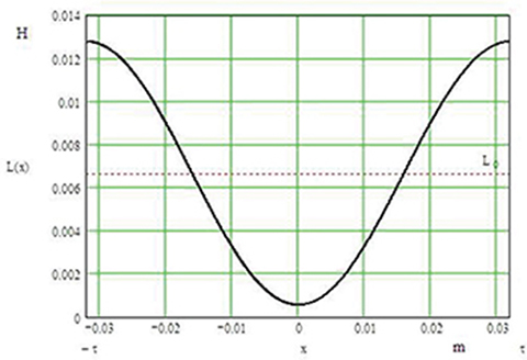
Fig. 3.11. Variation of inductance with armature position.

Images

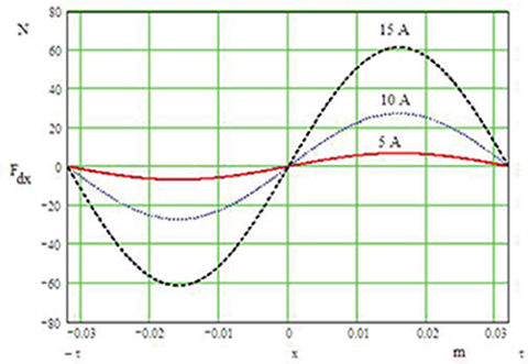
Fig. 3.12. Variation of electromagnetic thrust with armature position.

$F_{m a x} = \frac{1}{4} \frac{π}{0.032} 0.0011 = 0.273 N$

Variation of electromagnetic thrust with current and pole pitch according to eqn (3.126) is shown in Fig. 3.12. For I_a = 5 A, the thrust at 0.5τ = 16 mm is F_dx = 6.813 N; for I_a = 10 A, the thrust at 0.5τ = 16 mm is F_dx = 27.25 N; and for I_a = 15 A, the thrust at 0.5τ = 16 mm is F_dx = 61.32 N.

The presented method of approximate calculation of inductance and electromagnetic thrust does not include magnetic saturation, fringing and leakage flux, and can be used only for very rough estimation of the performance of an SR linear motor. Fringing and leakage fluxes can be included by using field plotting or dividing the magnetic field into simple solids as shown in Appendix B.

..................Content has been hidden....................

You can't read the all page of ebook, please click here login for view all page.

Table of Contents for
3 Theory of Linear Synchronous Motors

3

Theory of Linear Synchronous Motors

3.1 Permanent Magnet Synchronous Motors

3.1.1 Magnetic Field of the Armature Winding

3.1.2 Form Factors and Reaction Factors

3.1.3 Synchronous Reactance

3.1.4 Voltage Induced

3.1.5 Electromagnetic Power and Thrust

3.1.6 Minimization of d-axis Armature Current

3.1.7 Thrust Ripple

3.1.8 Magnetic Circuit

3.1.9 Direct Calculation of Thrust

3.2 Motors with Superconducting Excitation Coils

3.3 Double-Sided LSM with Inner Moving Coil

3.4 Variable Reluctance Motors

3.5 Switched Reluctance Motors

Examples

Table of Contents for 3 Theory of Linear Synchronous Motors

Create new playlist

Sign In

Sign Up

Table of Contents for
3 Theory of Linear Synchronous Motors