6 Motion Control

Search in book...
Toggle Font Controls
Create new playlist

Name your new playlist

Playlist description (optional)
Sign In

Email address

Password

Forgot Password?

or

Continue with Facebook

Continue with Google
Sign Up

Full Name

Email address

Confirm Email Address

Password

or

Continue with Facebook

Continue with Google

Control variables are classified into input variables (input voltage, input frequency), output variables (speed, angular displacement, torque), and internal variables (armature current, magnetic flux). The mathematical model of an a.c. motor is nonlinear, which for small variations of the input voltage, input frequency, and output speed can be linearized.

Scalar control methods are based on changing only the amplitudes of controlled variables. A typical example is to maintain constant torque (magnetic flux) of a.c. motors by keeping constant the V/f ratio. The scalar control can be implemented both in the open loop (most of industrial applications) and closed loop control systems with speed feedback.

In the vector oriented control method (Fig. 6.1), both the amplitudes and phases of the space vectors of variables are changed. Vector control based upon the field orientation principle uses the analogy between the a.c. (induction or synchronous) motor and the d.c. commutator motor. The active and reactive currents are decoupled, which, in turn, determine the thrust and magnetic flux, respectively.

Standard controllers have a fixed structure and constant parameters. However, the parameters of electric motors are variable, e.g., winding resistances are temperature dependent, and winding inductances are magnetic saturation dependent. Consequently, the deterioration of the dynamic behavior of the drive can even lead to its unstability. In adaptive controllers, variable parameters or structure are adjusted to the change in parameters of the drive system.

In a self-tuning adaptive control, the controller parameters are tuned to adapt to the drive parameter variation. In a model reference adaptive control, the drive response is forced to track the response of a reference model irrespective of the drive parameter variation. This can be achieved by storing the fixed parameter reference model in the computer memory. Some model reference control methods are based on search strategy.

Images

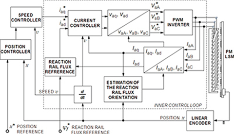
Fig. 6.1. Vector oriented control of an a.c. motor.

The sliding mode control is a variable structure control technique similar to the adaptive model reference control. In sliding mode control, the response of the drive system is insensitive to the parameter and load variations. Thus, this method is suitable for servo drives, e.g., machine tools, robots, factory automation systems, etc. The drive system is forced to “slide” along the so-called predefined trajectory in the state space by a switching control algorithm independently of change in its parameters and load.

The above classical control methods use a mathematical model of the controlled system either in the form of a transfer function or in the form of state space equations. Neural and fuzzy logic control are based on artificial intelligence and do not need any mathematical models.

Neural control applies an artificial neural network as a controller or emulator of the dynamic system. The artificial neural network is a network of artificial neurons that simulate the nervous system of the human brain. Each neuron in a single layer is connected with all neurons of the neighboring layers with the aid of so-called synapses¹. The neural controller with its associative property memory can create a nonlinear relationship between its input and output values. Since there is no flux estimator, the input–output relationship has to be trained on a sufficient number of samples. The training can be performed either online or offline.

A controller that is based on fuzzy logic uses the experience and intuition of a human plant operator. The memory of a fuzzy controller creates fuzzy logic rules, e.g., if the speed of an LSM is slow, and the reference speed is fast, then set the input signal (frequency) is high. The main advantage of fuzzy control is that a strictly nonlinear or unknown system can be controlled by linguistic variables. Plants that are difficult to model using conventional parameter identification techniques can be made controllable by implementing human expert knowledge.

6.2 EMF and Thrust of PM Synchronous and Brushless Motors

6.2.1 Sine-Wave Motors

A three-phase (multiphase) armature winding with distributed parameters produces sinusoidal or quasi-sinusoidal distribution of the MMF. For a sinusoidal distribution of the air gap magnetic flux density, the first harmonic of the excitation flux can be found on the basis of eqn (3.26). The excitation magnetic flux calculated on the basis of the maximum air gap magnetic flux density B_mg is then Φ_f ≈ Φ_f1 = (2/π)L_iτk_fB_mg, where the form factor of the excitation field k_f = B_mg1/B_mg is according to eqn (3.10). Assuming that the instantaneous value of the EMF induced in a single stator conductor by the first harmonic of the magnetic flux density is e_f1 = E_mf1 sin(ωt) = B_mg1L_iv_s sin(ωt) = 2fB_mg1L_iτ sin(ωt), the rms EMF is Emf1/2–√fBmg1Liτ=(1/2)π2–√f(2/π)Bmg1Liτ $E_{m f 1} / \sqrt{2} f B_{m g 1} L_{i} τ = (1 / 2) π \sqrt{2} f (2 / π) B_{m g 1} L_{i} τ$ . For two conductors or one turn, Emf1/2–√=π2–√f(2/π)Bmg1Liτ $E_{m f 1} / \sqrt{2} = π \sqrt{2} f (2 / π) B_{m g 1} L_{i} τ$ . For N₁k_w1 turns, where k_w1 is the winding factor, the rms EMF is

E f \approx E f 1 = π 2 - \sqrt f N 1 k w 1 α i k f B m g L i τ = π τ 1 2 \sqrt N 1 k w 1 Φ f υ s = c E Φ f υ s (6.1)

$\begin{matrix} E_{f} \approx E_{f 1} = π \sqrt{2} f N_{1} k_{w 1} α_{i} k_{f} B_{m g} L_{i} τ \\ = \frac{π}{τ} \frac{1}{\sqrt{2}} N_{1} k_{w 1} Φ_{f} υ_{s} = c_{E} Φ_{f} υ_{s} \end{matrix} (6.1)$

where 2/π is replaced by α_i and the EMF (armature) constant is

c E = π τ 1 2 - \sqrt N 1 k w 1 (6.2)

$c_{E} = \frac{π}{τ} \frac{1}{\sqrt{2}} N_{1} k_{w 1} (6.2)$

For Φ_f = const a new EMF constant

k E = c E Φ f (6.3)

$k_{E} = c_{E} Φ_{f} (6.3)$

can be used. Assuming a negligible difference between the d- and q-axis synchronous reactances, i.e., X_sd ≈ X_sq, the electromagnetic (air gap) power P_elm ≈ m₁E_fI_aq = m₁E_fI_a cos Ψ. Note that in academic textbooks the electromagnetic power is usually calculated neglecting the armature winding resistance R₁ as P_elm ≈ P_in = m₁V₁I_a cos ϕ = m₁V₁I_a cos(δ + Ψ), where cos((δ + Ψ) = E_f sin δ/(I_aX_sd). Putting E_f according to eqn (6.1) and v_s = 2fτ, the electromagnetic thrust developed by the LSM is

F d x = P e l m υ s = m 1 E f I a υ s = cos Ψ = m 1 π τ 1 2 \sqrt N 1 k w 1 Φ f I a cos Ψ = m 1 2 c F Φ f I a cos Ψ (6.4)

$\begin{matrix} F_{d x} = \frac{P_{e l m}}{υ_{s}} = \frac{m_{1} E_{f} I_{a}}{υ_{s}} = \cos Ψ \\ = m_{1} \frac{π}{τ} \frac{1}{\sqrt{2}} N_{1} k_{w 1} Φ_{f} I_{a} \cos Ψ = \frac{m_{1}}{2} c_{F} Φ_{f} I_{a} \cos Ψ \end{matrix} (6.4)$

where the thrust constant is

c F = 2 c E = π 2 - \sqrt τ N 1 k w 1 (6.5)

$c_{F} = 2 c_{E} = \frac{π \sqrt{2}}{τ} N_{1} k_{w 1} (6.5)$

For Φ_f = const a new thrust constant

k F = c F Φ f (6.6)

$k_{F} = c_{F} Φ_{f} (6.6)$

simplifies prediction of thrust-current characteristics. The maximum thrust

F d x m a x = m 1 2 c F Φ f I a = m 1 2 k E I a (6.7)

$F_{d x m a x} = \frac{m_{1}}{2} c_{F} Φ_{f} I_{a} = \frac{m_{1}}{2} k_{E} I_{a} (6.7)$

is for the angle Ψ = 0°, which means that δ = ϕ (Fig. 6.2). In such a case, there is no demagnetizing component Φ_ad of the armature reaction flux and the air gap magnetic flux density takes its maximum value. The EMF E_f is high so it can better balance the input voltage V₁, thus minimizing the armature current I_a. When Ψ ≈ 0⁰, the low armature current I_a ≈ I_aq is mainly torque producing. An angle Ψ = 0⁰ results in a decoupling of the rotor flux Φ_f and the armature flux Φ_a.

Images

Fig. 6.2. Phasor diagram at I_ad = 0.

Images

Fig. 6.3. IGBT inverter-fed armature circuits of PM LBMs: (a) Y-connected phase windings, (b) Δ-connected armature windings.

6.2.2 Square-Wave (Trapezoidal) Motors

PM LBMs predominantly have the reaction rail designed with surface PMs and large effective pole-arc coefficient α(sq)i=bp/τ $α_{i}^{(s q)} = b_{p} / τ$ . The three-phase armature winding with distributed parameters can be Y, or Δ-connected. For the Y-connected winding, as in Fig. 6.3, two phases conduct the armature current at the same time.

For a.c. synchronous motors [70],

V 1 = E f + I a d (R 1 + j X s d) + I a q (R 1 + j X s q) (6.8)

$V_{1} = E_{f} + I_{a d} (R_{1} + j X_{s d}) + I_{a q} (R_{1} + j X_{s q}) (6.8)$

Rectangular (trapezoidal) waveforms in the armature winding of an inverter-fed LBM correspond to the operation of a d.c. commutator motor. For a d.c. motor ω → 0, then eqn (6.8) becomes

V = E f + R I (s q) a (6.9)

$V = E_{f} + R I_{a}^{(s q)} (6.9)$

where R is the sum of two-phase resistances in series (for Y-connected phase windings), and E_f is the sum of two-phase EMFs in series, V is the d.c. input voltage supplying the inverter, and I(sq)a $I_{a}^{(s q)}$ is the flat-top value of the square-wave current equal to the inverter input current.

For an ideal rectangular distribution of B_mg = const in the interval of 0 ≤ x ≤ τ or from 0 to 180 electrical degrees

Φ (s q) f = L i \int τ 0 B m g d x = τ L i B m g

$Φ_{f}^{(s q)} = L_{i} \int_{0}^{τ} B_{m g} d x = τ L_{i} B_{m g}$

Including the pole shoe width b_p < τ and a fringing flux, the excitation flux is somewhat smaller:

Φ (s q) f = b p L i B m g = α (s q) i τ L i B m g (6.10)

$Φ_{f}^{(s q)} = b_{p} L_{i} B_{m g} = α_{i}^{(s q)} τ L_{i} B_{m g} (6.10)$

For a rectangular (trapezoidal) wave excitation, the EMF induced in a single turn (two conductors) is 2B_mgL_iv = 4fB_mgL_iτ. Including b_p and fringing flux, the EMF for N₁k_w₁ turns ef=4fN1kw1α(sq)iτLiBmg=4fN1kw1Φ(sq)f $e_{f} = 4 f N_{1} k_{w 1} α_{i}^{(s q)} τ L_{i} B_{m g} = 4 f N_{1} k_{w 1} Φ_{f}^{(s q)}$ . For the Y-connection of the armature windings, as in Fig. 6.3a, two phases are conducting at the same time. The EMF contributing to the electromagnetic power is

E f = 2 e f = 8 f N 1 k w 1 α (s q) i τ L i B m g = 4 τ N 1 k w 1 Φ (s q) f υ = c E d c Φ (s q) f υ = k E d c υ (6.11)

$E_{f} = 2 e_{f} = 8 f N_{1} k_{w 1} α_{i}^{(s q)} τ L_{i} B_{m g} = \frac{4}{τ} N_{1} k_{w 1} Φ_{f}^{(s q)} υ = c_{E d c} Φ_{f}^{(s q)} υ = k_{E d c} υ (6.11)$

where the EMF constants are

c E d c = 4 τ N 1 k w 1 (6.12)

$c_{E d c} = \frac{4}{τ} N_{1} k_{w 1} (6.12)$

and

k E d c = c E d c Φ (s q) f (6.13)

$k_{E d c} = c_{E d c} Φ_{f}^{(s q)} (6.13)$

The electromagnetic thrust developed by the LSM is expressed by the equation

F d x = P g υ = E f I ( s q ) a υ = 4 τ N 1 k w 1 Φ (s q) f = c F d c Φ (s q) f I (s q) a = k F d c I (s q) a (6.14)

$F_{d x} = \frac{P_{g}}{υ} = \frac{E_{f} I_{a}^{(s q)}}{υ} = \frac{4}{τ} N_{1} k_{w 1} Φ_{f}^{(s q)} = c_{F d c} Φ_{f}^{(s q)} I_{a}^{(s q)} = k_{F d c} I_{a}^{(s q)} (6.14)$

in which

c F d c = c E d c; k F d c = c F d c Φ (s q) f (6.15)

$\begin{matrix} c_{F d c} = c_{E d c}; & k_{F d c} = c_{F d c} Φ_{f}^{(s q)} \end{matrix} (6.15)$

and I(sq)a $I_{a}^{(s q)}$ is the flat-top value of the phase current. Eqn (6.14) indicates that the thrust developed by the PM LBM can be controlled directly by varying the current.

For v = v_s and Ψ = 0° the ratio F_dx of a square-wave motor to F_dx of a sinewave motor is

F ( s q ) d x F d x = 4 2 - \sqrt π m 1 Φ ( s q ) f Φ f I ( s q ) a I a (6.16)

$\frac{F_{d x}^{(s q)}}{F_{d x}} = \frac{4 \sqrt{2}}{π m_{1}} \frac{Φ_{f}^{(s q)}}{Φ_{f}} \frac{I_{a}^{(s q)}}{I_{a}} (6.16)$

For three-phase motors,

F ( s q ) d x F d x = 4 2 - \sqrt π m 1 Φ ( s q ) f Φ f I ( s q ) a I a (6.17)

$\frac{F_{d x}^{(s q)}}{F_{d x}} = \frac{4 \sqrt{2}}{π m_{1}} \frac{Φ_{f}^{(s q)}}{Φ_{f}} \frac{I_{a}^{(s q)}}{I_{a}} (6.17)$

6.3 Model of PM Motor in dq Reference Frame

Control algorithms of sinusoidally excited synchronous motors frequently use the d-q model of synchronous machines. The d-q dynamic model is expressed in a rotating reference frame that moves at synchronous speed ω. The time-varying parameters are eliminated, and all variables are expressed in orthogonal or mutually decoupled d and q axes.

A synchronous machine is described by the following set of differential equations:

υ 1 d = R 1 i a d + d ψ d d t - w ψ q (6.18)

$υ_{1 d} = R_{1} i_{a d} + \frac{d ψ_{d}}{d t} - w ψ_{q} (6.18)$

υ 1 q = R 1 i a q + d ψ q d t - w ψ d (6.19)

$υ_{1 q} = R_{1} i_{a q} + \frac{d ψ_{q}}{d t} - w ψ_{d} (6.19)$

υ f = R f I f + d ψ f d t (6.20)

$υ_{f} = R_{f} I_{f} + \frac{d ψ_{f}}{d t} (6.20)$

0 = R D i D + d ψ D d t (6.21)

$0 = R_{D} i_{D} + \frac{d ψ_{D}}{d t} (6.21)$

0 = R Q i Q + d ψ Q d t (6.22)

$0 = R_{Q} i_{Q} + \frac{d ψ_{Q}}{d t} (6.22)$

The linkage fluxes in the above equations are defined as

ψ d = (L a d + L 1) i a d + L a d i D + ψ f = L s d i a d + L a d i D + ψ f (6.23)

$ψ_{d} = (L_{a d} + L_{1}) i_{a d} + L_{a d} i_{D} + ψ_{f} = L_{s d} i_{a d} + L_{a d} i_{D} + ψ_{f} (6.23)$

ψ d = (L a q + L 1) i a q + L a q i Q = L s q i a q + L a q i Q (6.24)

$ψ_{d} = (L_{a q} + L_{1}) i_{a q} + L_{a q} i_{Q} = L_{s q} i_{a q} + L_{a q} i_{Q} (6.24)$

ψ f = L a d i a d + (L a d + L l f) i f d + L a d i D (6.25)

$ψ_{f} = L_{a d} i_{a d} + (L_{a d} + L_{l f}) i_{f d} + L_{a d} i_{D} (6.25)$

ψ D = L a d i a d + (L a d + L D) i D + ψ f (6.26)

$ψ_{D} = L_{a d} i_{a d} + (L_{a d} + L_{D}) i_{D} + ψ_{f} (6.26)$

ψ Q = L a q i a q + (L a q + L Q) i Q (6.27)

$ψ_{Q} = L_{a q} i_{a q} + (L_{a q} + L_{Q}) i_{Q} (6.27)$

where v_1d and v_1q are d- and q-axis components of terminal voltage, ψ_f is the maximum flux linkage per phase produced by the excitation system; R₁ is the armature winding resistance; L_ad, L_aq are d- and q-axis components of the armature self-inductance, respectively; ω = πv_s/τ is the angular frequency of the armature current; τ is the pole pitch; v_s is the linear synchronous velocity; i_ad, i_aq are the d- and q-axis components of the armature current, respectively; i_D, i_Q are d- and q-axis components of the damper current, respectively. The field winding resistance, which exists only in the case of electromagnetic excitation, is R_f, the field excitation current is I_f, the excitation linkage flux is ψ_f, and the field leakage inductance is L_lf. The damper resistance and inductance in the d-axis are R_D and L_D, respectively. The damper resistance and inductance in the q-axis are R_Q and L_Q, respectively. The resultant armature inductances are

L s d = L a d + L 1, L s q = L a q + L 1 (6.28)

$\begin{matrix} L_{s d} = L_{a d} + L_{1}, & L_{s q} = L_{a q} + L_{1} \end{matrix} (6.28)$

where L_ad and L_aq are self-inductances in the d and q-axis, respectively, and L₁ is the leakage inductance of the armature winding per phase. In a three-phase machine, L_ad = (3/2)L′_ad and L_aq = (3/2)L′_aq, where L′_ad and L′_aq are self-inductances of a single-phase machine.

The excitation linkage flux in eqn (6.25) is (L_ad + L_lf)i_fd, while L_adi_ad is the armature reaction flux. In the case of a PM field excitation, the fictitious current (equivalent MMF) is I_f = H_ch_M and ifd=2–√If $i_{f d} = \sqrt{2} I_{f}$ .

For no damper winding, i.e., i_D = i_Q = 0, the voltage equations in the d-and q-axis are

υ 1 d = R 1 i a d + d ψ d d t - w ψ q = (R 1 + d L s d d t) i a d - w L s q i a q (6.29)

$υ_{1 d} = R_{1} i_{a d} + \frac{d ψ_{d}}{d t} - w ψ_{q} = (R_{1} + \frac{d L_{s d}}{d t}) i_{a d} - w L_{s q} i_{a q} (6.29)$

υ 1 q = R 1 i a q + d ψ q d t + w ψ d = (R 1 + d L s q d t) i a q + w L s d i a d + w ψ f (6.30)

$υ_{1 q} = R_{1} i_{a q} + \frac{d ψ_{q}}{d t} + w ψ_{d} = (R_{1} + \frac{d L_{s q}}{d t}) i_{a q} + w L_{s d} i_{a d} + w ψ_{f} (6.30)$

The matrix form of voltage equations in terms of inductances L_sd and L_sq is

[υ 1 d υ 1 q] = [R 1 + d d t L s d w L s d - w L s q R 1 + d d t L s q] [i a d i a q] + [0 w ψ f] (6.31)

$[\begin{matrix} υ_{1 d} \\ υ_{1 q} \end{matrix}] = [\begin{matrix} R_{1} + \frac{d}{d t} L_{s d} & - w L_{s q} \\ w L_{s d} & R_{1} + \frac{d}{d t} L_{s q} \end{matrix}] [\begin{matrix} i_{a d} \\ i_{a q} \end{matrix}] + [\begin{matrix} 0 \\ w ψ_{f} \end{matrix}] (6.31)$

For the steady-state operation (d/dt)L_sdi_ad = (d/dt)L_sqi_aq = 0, I_a = I_ad + jI_aq, V₁ + jV_1q, iad=2–√Iad,iaq=2–√Iaq,v1d=2–√V1d,v1q=2–√V1q,Ef=ωLfdIf/2–√=ωψf/2–√ $i_{a d} = \sqrt{2} I_{a d}, i_{a q} = \sqrt{2} I_{a q}, v_{1 d} = \sqrt{2} V_{1 d}, v_{1 q} = \sqrt{2} V_{1 q}, E_{f} = ω L_{f d} I_{f} / \sqrt{2} = ω ψ_{f} / \sqrt{2}$ [60]. The quantities ωL_sd and ωL_sq are known as the d- and q-axis synchronous reactances, respectively. Eqn (6.31) can be brought to the form (3.32).

The instantaneous power input to the three-phase armature is

p i n = υ 1 A i a A + υ 1 B i a B + υ 1 C i a C = 3 2 (υ 1 d i a d + υ 1 q i a q) (6.32)

$p_{i n} = υ_{1} A^{i} a A + υ_{1} B^{i} a B + υ_{1} C^{i} a C = \frac{3}{2} (υ_{1 d} i_{a d} + υ_{1 q} i_{a q}) (6.32)$

The power balance equation is obtained from eqns (6.29) and (6.30), i.e.,

υ 1 d i a d + υ 1 q i a q = R 1 i 2 a d + d ψ d d t i a d + R 1 i 2 a q + d ψ q d t i a q + w (ψ d i a q - ψ q i a d) (6.33)

$υ_{1 d} i_{a d} + υ_{1 q} i_{a q} = R_{1} i_{a d}^{2} + \frac{d ψ_{d}}{d t} i_{a d} + R_{1} i_{a q}^{2} + \frac{d ψ_{q}}{d t} i_{a q} + w (ψ_{d} i_{a q} - ψ_{q} i_{a d}) (6.33)$

The last term ω(ψ_di_aq − ψ_qi_ad) accounts for the electromagnetic power of a single-phase, two-pole synchronous machine. For a three-phase machine

p e l m = 3 2 w (ψ d i a q - ψ q i a d) = 3 2 w [(L s d i a d + ψ f) i a q - L s q i a d i a q] = 3 2 w [ψ f + (L s d - L s q) i a d] i a q (6.34)

$\begin{matrix} p_{e l m} = \frac{3}{2} w (ψ_{d} i_{a q} - ψ_{q} i_{a d}) = \frac{3}{2} w [(L_{s d} i_{a d} + ψ_{f}) i_{a q} - L_{s q} i_{a d} i_{a q}] \\ = \frac{3}{2} w [ψ_{f} + (L_{s d} - L_{s q}) i_{a d}] i_{a q} \end{matrix} (6.34)$

The electromagnetic thrust of a three-phase LSM is

F d x = p e l m υ s = 3 2 π τ [ψ f + (L s d - L s q) i a d] i a q N (6.35)

$\begin{matrix} F_{d x} = \frac{p_{e l m}}{υ_{s}} = \frac{3}{2} \frac{π}{τ} [ψ_{f} + (L_{s d} - L_{s q}) i_{a d}] i_{a q} & N \end{matrix} (6.35)$

where v_s = 2fτ = ωτ/π. Compare eqn (6.35) with eqn (3.41).

The relationships between i_ad, i_aq and phase currents i_aA, i_aB, and i_aC are,

i a d = 2 3 [i a A cos w t + i a B cos (w t + 2 π 3) + i a C cos (w t + 2 π 3)] (6.36)

$i_{a d} = \frac{2}{3} [i_{a A} \cos w t + i_{a B} \cos (w t + \frac{2 π}{3}) + i_{a C} \cos (w t + \frac{2 π}{3})] (6.36)$

i a q = - 2 3 [i a A sin w t + i a B sin (w t - 2 π 3) + i a C sin (w t + 2 π 3)] (6.37)

$i_{a q} = - \frac{2}{3} [i_{a A} \sin w t + i_{a B} \sin (w t - \frac{2 π}{3}) + i_{a C} \sin (w t + \frac{2 π}{3})] (6.37)$

The reverse relations, obtained by simultaneous solution of eqns (6.36) and (6.37) in conjunction with i_aA + i_aB + i_aC = 0, are

i a A = i a d cos w t - i a q sin w t i a B = i a d cos (w t - 2 π 3) - i a q sin (w t - 2 π 3) i a C = i a d cos (w t + 2 π 3) - i a q sin (w t + 2 π 3) (6.38)

$\begin{matrix} i_{a A} = i_{a d} \cos w t - i_{a q} \sin w t \\ i_{a B} = i_{a d} \cos (w t - \frac{2 π}{3}) - i_{a q} \sin (w t - \frac{2 π}{3}) \\ i_{a C} = i_{a d} \cos (w t + \frac{2 π}{3}) - i_{a q} \sin (w t + \frac{2 π}{3}) \end{matrix} (6.38)$

Including the zero-sequence current

i 0 = 1 3 (i a A + i a B + I a C) (6.39)

$i_{0} = \frac{1}{3} (i_{a A} + i_{a B} + I_{a C}) (6.39)$

the relationship between dq0 and ABC currents can be written in the following matrix form:

⎡ ⎣ ⎢ i a d i a q i 0 ⎤ ⎦ ⎥ = 2 3 ⎡ ⎣ ⎢ ⎢ ⎢ cos (ω t) - sin (ω t) 1 2 cos (ω t - 2 π 3) - sin (ω t - 2 π 3) 1 2 cos (ω t + 2 π 3) - sin (ω t + 2 π 3) 1 2 ⎤ ⎦ ⎥ ⎥ ⎥

$[\begin{matrix} i_{a d} \\ i_{a q} \\ i_{0} \end{matrix}] = \frac{2}{3} [\begin{matrix} \cos (ω t) & \cos (ω t - \frac{2 π}{3}) & \cos (ω t + \frac{2 π}{3}) \\ - \sin (ω t) & - \sin (ω t - \frac{2 π}{3}) & - \sin (ω t + \frac{2 π}{3}) \\ \frac{1}{2} & \frac{1}{2} & \frac{1}{2} \end{matrix}]$

\times ⎡ ⎣ ⎢ i a A i a B i a C ⎤ ⎦ ⎥ = [B] ⎡ ⎣ ⎢ i a A i a B i a C ⎤ ⎦ ⎥ (6.40)

$\times [\begin{matrix} i_{a A} \\ i_{a B} \\ i_{a C} \end{matrix}] = [B] [\begin{matrix} i_{a A} \\ i_{a B} \\ i_{a C} \end{matrix}] (6.40)$

where

[B] = 2 3 ⎡ ⎣ ⎢ ⎢ ⎢ cos (w t) - sin (w t) 1 2 cos (w t - 2 π 3) - sin (w t - 2 π 3) 1 2 cos (w t + 2 π 3) - sin (w t + 2 π 3) 1 2 ⎤ ⎦ ⎥ ⎥ ⎥ (6.41)

$[B] = \frac{2}{3} [\begin{matrix} \cos (w t) & \cos (w t - \frac{2 π}{3}) & \cos (w t + \frac{2 π}{3}) \\ - \sin (w t) & - \sin (w t - \frac{2 π}{3}) & - \sin (w t + \frac{2 π}{3}) \\ \frac{1}{2} & \frac{1}{2} & \frac{1}{2} \end{matrix}] (6.41)$

is the transformation matrix originally proposed by Blondel [57]. This is not a power invariant transformation matrix. The inverse transformation takes the form

⎡ ⎣ ⎢ i a A i a B i a C ⎤ ⎦ ⎥ = ⎡ ⎣ ⎢ ⎢ cos (w t) cos (w t - 2 π 3) cos (w t + 2 π 3) - sin (w t) - sin (w t - 2 π 3) - sin (w t + 2 π 3) 111 ⎤ ⎦ ⎥ ⎥ ⎡ ⎣ ⎢ i a d i a q i 0 ⎤ ⎦ ⎥ = [B] - 1 ⎡ ⎣ ⎢ i a d i a q i 0 ⎤ ⎦ ⎥ (6.42)

$[\begin{matrix} i_{a A} \\ i_{a B} \\ i_{a C} \end{matrix}] = [\begin{matrix} \cos (w t) & - \sin (w t) & 1 \\ \cos (w t - \frac{2 π}{3}) & - \sin (w t - \frac{2 π}{3}) & 1 \\ \cos (w t + \frac{2 π}{3}) & - \sin (w t + \frac{2 π}{3}) & 1 \end{matrix}] [\begin{matrix} i_{a d} \\ i_{a q} \\ i_{0} \end{matrix}] = {[B]}^{- 1} [\begin{matrix} i_{a d} \\ i_{a q} \\ i_{0} \end{matrix}] (6.42)$

The inverse² of Blondel’s transformation matrix

[B] - 1 = ⎡ ⎣ ⎢ ⎢ cos (w t) cos (w t - 2 π 3) cos (w t + 2 π 3) - sin (w t) - sin (w t - 2 π 3) - sin (w t + 2 π 3) 111 ⎤ ⎦ ⎥ ⎥ (6.43)

${[B]}^{- 1} = [\begin{matrix} \cos (w t) & - \sin (w t) & 1 \\ \cos (w t - \frac{2 π}{3}) & - \sin (w t - \frac{2 π}{3}) & 1 \\ \cos (w t + \frac{2 π}{3}) & - \sin (w t + \frac{2 π}{3}) & 1 \end{matrix}] (6.43)$

Similar equations as (6.40) and (6.42) can be written for voltages and magnetic fluxes.

The transpose³ of Blondel’s transformation matrix (6.41)

[B] T = ⎡ ⎣ ⎢ ⎢ ⎢ cos (w t) cos (w t - 2 π 3) cos (w t + 2 π 3) - sin (w t) - sin (w t - 2 π 3) - sin (w t + 2 π 3) 1 2 1 2 1 2 ⎤ ⎦ ⎥ ⎥ ⎥ (6.44)

${[B]}^{T} = [\begin{matrix} \cos (w t) & - \sin (w t) & \frac{1}{2} \\ \cos (w t - \frac{2 π}{3}) & - \sin (w t - \frac{2 π}{3}) & \frac{1}{2} \\ \cos (w t + \frac{2 π}{3}) & - \sin (w t + \frac{2 π}{3}) & \frac{1}{2} \end{matrix}] (6.44)$

The power input is proportional to the sum v_1Ai_aA + v_1Bi_aB + v_1Ci_aC, i.e.,

p i n = υ 1 A i a A + υ 1 B i a B + υ 1 C i a C = [υ 1 A υ 1 B υ 1 C] ⎡ ⎣ ⎢ i a A i a B i a C ⎤ ⎦ ⎥ (6.45)

$p_{i n} = υ_{1 A} i_{a A} + υ_{1 B} i_{a B} + υ_{1 C} i_{a C} = [υ_{1 A} υ_{1 B} υ_{1 C}] [\begin{matrix} i_{a A} \\ i_{a B} \\ i_{a C} \end{matrix}] (6.45)$

Putting v_1A, v_1B, v_1C and i_aA, i_aB, i_aC from eqn (6.42), the power is

p i n = 3 2 (υ 1 d i a d + υ 1 q i a q + 2 υ 0 i 0) = [υ 1 d υ 1 q 2 υ 0] ⎡ ⎣ ⎢ i a d i a q i 0 ⎤ ⎦ ⎥ (6.46)

$p_{i n} = \frac{3}{2} (υ_{1 d} i_{a d} + υ_{1 q} i_{a q} + 2 υ_{0} i_{0}) = [υ_{1 d} υ_{1 q} 2 υ_{0}] [\begin{matrix} i_{a d} \\ i_{a q} \\ i_{0} \end{matrix}] (6.46)$

According to Park [165], the proportionality coefficient must be 3/2 for any instant during normal operation at unity power factor.

6.4 Thrust and Speed Control of PM Motors

Thrust-speed envelopes of PM LSMs are classified into two categories: constant thrust (Fig. 6.4a) and constant power (Fig. 6.4b).

For constant thrust requirements, the thrust-speed envelope is of a rectangular shape. The maximum thrust F_xmax should be obtained at all linear speeds up to the speed v_b. Such envelope is required for linear servo drives and actuators.

For constant power requirements, the thrust-speed envelope is of a hyperbolic shape because F_xv = P_out = const. The constant power trajectory is maintained over a wide speed range from the base speed v_b to the maximum speed v_max. Such envelope is required for traction linear motors that are used in, e.g., linear-motor-driven vehicles. A constant power operation is implemented by weakening the excitation flux. Since PM motors do not have field excitation windings, the magnetic flux is weakened by applying appropriate control techniques. It can also be done by a hardware, i.e., using a hybrid excitation system that consists of PMs and additional excitation coils placed around PMs.

Images

Fig. 6.4. Thrust-speed envelopes of LSMs: (a) constant thrust, (b) constant power.

Control algorithms are, in prinicple, similar for both sine-wave and square-wave PM motors. Fig. 6.5 shows how control loops can be developed to achieve thrust, speed and position control in motion control systems with PM LSMs. These cascaded control structures (Fig. 6.5) for LSMs have been based on control structures for rotary PM synchronous motors [98].

The following are some examples of control of PM LSMs and LBMs.

Images

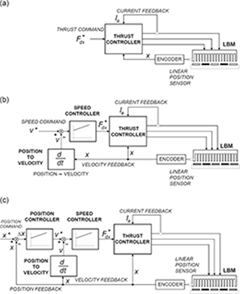
Fig. 6.5. Cascaded control loops for PM LSMs: (a) current-regulated thrust control, (b) velocity and thrust control, (c) position, velocity, and current control.

6.4.1 Open Loop Control

Aluminum shields or mild-steel pole shoes of surface PM LSMs are equivalent to damper cage windings. Solid steel poles of buried PMs behave also as dampers. A damper adds a component of asynchronous thrust production so that the PM LSM can be operated stably from an inverter without position sensors. As a result, a simple constant voltage-to-frequency control algorithm (Fig. 6.6) can provide speed control for applications that do not require fast dynamic response. Thus, PM LSM motors can replace LIMs in some variable-speed drives to improve the drive efficiency with minimal changes to the control electronics.

6.4.2 Closed Loop Control

To achieve high performance motion control with a PM LSM, a position sensor is typically required. The rotor position feedback needed to continuously perform the self-synchronization function for a sinusoidal PM motor is significantly more demanding than that for a square-wave motor. An absolute encoder or resolver is typically required. The second condition for achieving high-performance motion control is high-quality phase current control.

Images

Fig. 6.6. Simplified block diagram of open loop voltage-to-frequency control of a PM LSM with damper.

Images

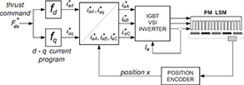
Fig. 6.7. Block diagram of high-performance thrust control scheme for PM LSM using vector control concept.

One of the possible approaches is the vector control shown in Fig. 6.7. The incoming thrust command F∗dx $F_{d x}^{*}$ is mapped into commands for i∗ad $i_{a d}^{*}$ and i∗aq $i_{a q}^{*}$ current components according to eqn (6.35).

The current commands in the moving reaction rail d-q reference frame (seen as d.c. quantities for a constant thrust command) are then transformed into the instantaneous sinusoidal current commands for the individual armature phases i∗aA,i∗aB $i_{a A}^{*}, i_{a B}^{*}$ , and i∗aC $i_{a C}^{*}$ using the reaction rail or armature position feedback and reverse Park’s transformation equations [60, 96]. Current regulators for each of the three armature current phases then operate to excite the phase windings with the desired current amplitudes. The most common means of mapping the thrust command F∗dx $F_{d x}^{*}$ into values for i∗ad $i_{a d}^{*}$ and i∗aq $i_{a q}^{*}$ is to set a constraint of maximum thrust-to-current operation that is nearly equivalent to maximizing operating efficiency [97].

6.4.3 Zero Direct-Axis Current Control

To obtain the thrust proportional to the armature current i_a = i_aq and free from the demagnetization of PMs, the PM LSM is driven by the d-axis current i_ad = 0 control, i.e.,

F d x = 3 2 p π τ ψ f i a q N (6.47)

$\begin{matrix} F_{d x} = \frac{3}{2} p \frac{π}{τ} ψ_{f} i_{a q} & N \end{matrix} (6.47)$

This means that the angle Ψ between the armature current and q-axis always remains 0° (see the phasor diagram in Fig. 6.2). Eqn (6.47) can also be simply derived assuming sinusoidal space distribution of the excitation magnetic flux density and sinusoidal time-varying armature currents including appropriate phase shifts.

6.4.4 Flux-Weakening Control

High coercivity rare-earth PMs are not affected by the armature reaction flux, and they cannot be permanently demagnetized by the armature flux. The d-axis reaction flux can be used for weakening the flux Φ_f produced by PMs. The flux-weakening control is similar to the field weakening control of d.c. commutator motors. In PM LSMs, the angle Ψ between the armature current and the q-axis is controlled. The drawback of this control technique is a decrease in the motor efficiency.

The armature current i_a is limited by the maximum current i_amax, i.e.,

i a = i 2 a d + i 2 a q - - - - - - - \sqrt \leq i a m a x (6.48)

$i_{a} = \sqrt{i_{a d}^{2} + i_{a q}^{2}} \leq i_{a m a x} (6.48)$

The maximum current i_amax is a continuous rated armature current for continuous duty cycle or a maximum available current of the inverter during short-time duty cycle [182].

The terminal voltage v₁ is limited by the maximum voltage v_1max, i.e.,

υ 1 = υ 2 1 d + υ 2 1 q - - - - - - - \sqrt \leq υ 1 m a x (6.49)

$υ_{1} = \sqrt{υ_{1 d}^{2} + υ_{1 q}^{2}} \leq υ_{1 m a x} (6.49)$

The maximum voltage v_1max is the maximum available output voltage of the inverter, which depends on the d.c. link voltage [182].

According to eqns (3.41) and (6.35), the thrust has two components: synchronous and reluctance thrust. Fig. 6.8 shows the thrust components of the LSM versus angle Ψ for the flux-weakening control. The synchronous thrust is proportional to cos Ψ with maximum at Ψ = 0°. The reluctance thrust takes its maximum value at Ψ = 45°. There is a critical angle Ψ_cr that corresponds to the maximum total thrust. The critical angle Ψ > 0 only if the reluctance thrust is produced. In an LSM with X_sd ≠ X_sq the maximum thrust for Ψ_cr > 0 is greater than the thrust for i_ad = 0 (Ψ = 0⁰) control.

The thrust-speed characteristics of an LSM for i_ad = 0 control and flux-weakening control are shown in Fig. 6.9.

Images

Fig. 6.8. Thrust plotted against the angle Ψ: 1 — synchronous thrust, 2 — reluctance thrust, 3 — total thrust.

Images

Fig. 6.9. Thrust–speed characteristics: 1 — i_ad = 0 control, 2 — flux-weakening control.

6.4.5 Direct Thrust Control

The basic idea of the direct thrust control (DTC) is to calculate the armature linkage flux directly from the electromagnetic induction law. The space phasor form of the armature voltage equation in the stationary reference frame is

v 1 = R 1 i a + d ψ d t (6.50)

$v_{1} = R_{1} i_{a} + \frac{d ψ}{d t} (6.50)$

The armature linkage flux can be found as [115, 254]

ψ = ψ 0 + \int t 1 t 0 (v 1 - R 1 i a) d t (6.51)

$ψ = ψ_{0} + \int_{t_{0}}^{t_{1}} (v_{1} - R_{1} i_{a}) d t (6.51)$

Since the armature linkage flux is calculated as an integral, an initial value of the armature linkage flux ψ₀ is required. The initial value is

ψ 0 = ψ f exp [j (900 \pm Ψ)]

$ψ_{0} = ψ_{f} \exp [j (90^{0} \pm Ψ)]$

where ψ_f is the PM flux to be estimated, and (90° ± Ψ) is the angle between the armature and excitation linkage fluxes.

Only the armature resistance R₁, space phasor of the armature voltage vector v₁ and space phasor of the armature current i_a is needed to find the armature linkage flux. This online integration (6.51) can be made with the aid of a high-speed DSP.

Eqn (6.51) shows that the variation of flux ψ depends on the voltage phasor v₁. Thus, the flux can be controlled using the voltage phasor. In DTC, an optimum voltage phasor that makes the flux rotate and produce the desired thrust needs to be chosen.

Each voltage phasor is constant during each switching interval, and eqn (6.51) can be written as

ψ = ψ 0 + v 1 t - R 1 \int t t 0 i a d t (6.52)

$ψ = ψ_{0} + v_{1} t - R_{1} \int_{t_{0}}^{t} i_{a} d t (6.52)$

If R₁ is negligible, the armature linkage flux ψ will be following the voltage phasor v₁.

In induction motors, when v₁ = 0, the armature linkage flux ψ is in a stationary position. In PM LSMs at v₁ = 0, the armature flux ψ is not stationary, because there is a relative motion between the armature and the excitation system. Zero voltage phasors cannot be used to control the rotation of ψ of PM LSMS.

The thrust of PM LSMs can be controlled by controlling the angle (90⁰±Ψ) between the armature and excitation linkage fluxes [115].

Depending on whether the actual thrust is smaller or larger than the reference thrust, the voltage phasors turn the linkage flux in the appropriate direction to increase or decrease the angle (90⁰± Ψ) and the thrust. The armature linkage flux always rotates in the direction determined by the output of the hysteresis controller of the thrust [115].

The linkage fluxes ψ_d(k) and ψ_q(k) at the kth sampling instant are

ψ d k = ψ d k - 1 + (υ 1 d k - 1 - R 1 i a d) t s (6.53)

$ψ_{d k} = ψ_{d k - 1} + (υ_{1 d k - 1} - R_{1} i_{a d}) t_{s} (6.53)$

ψ q k = ψ q k - 1 + (υ 1 q k - 1 - R 1 i a q) t s (6.54)

$ψ_{q k} = ψ_{q k - 1} + (υ_{1 q k - 1} - R_{1} i_{a q}) t_{s} (6.54)$

ψ k = ψ 2 d k + ψ 2 q k - - - - - - - - \sqrt (6.55)

$ψ_{k} = \sqrt{ψ_{d k}^{2} + ψ_{q k}^{2}} (6.55)$

where the subscript k − 1 denotes previous samples, and t_s is the sampling period.

Images

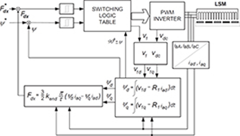
Fig. 6.10. Block diagram of direct thrust control of a PM LSM.

The electromagnetic thrust of an LSM is expressed by eqn (6.35). The end effect can be included by multiplying the thrust by a coefficient k_end < 1 that takes into account thrust reduction due to the end effect. Thus

F d x = 3 2 p k e n d π τ (ψ d i a q - ψ q i a d) (6.56)

$F_{d x} = \frac{3}{2} p k_{e n d} \frac{π}{τ} (ψ d i_{a q} - ψ_{q} i_{a d}) (6.56)$

The i_ad and i_aq currents are obtained from the measured three-phase currents i_aA, i_aB, i_aC, and the v_1d and v_1q voltages are calculated on the basis of the d.c. link voltage. The block diagram of the DTC control is shown in Fig. 6.10 [115].

6.4.6 Fuzzy Control

Fuzzy control of a PM LSM or LBM can be implemented according to the block diagram shown in Fig. 6.11. Two fuzzy controllers have been applied: for position and for speed control. A vector control is used in the power circuit with a current-controlled VSI.

6.5 Control of Hybrid Stepping Motors

6.5.1 Microstepping

When a stepping motor is driven in its full-stepping mode and two phases are energized simultaneously (Fig. 6.12a), the thrust available on each step is approximately the same. In the half-stepping mode, two phases and then only one are energized (Fig. 6.12b). If there is the same current in full-stepping and half-stepping modes, in each case a greater thrust is produced where two phases are energized simultaneously. This means that stronger thrust and weaker thrust are produced in each alternate step. The useful thrust is limited by the weaker step; however, there will be a reduction of low-speed pulsations over the full-step mode.

Images

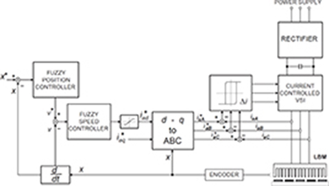
Fig. 6.11. Fuzzy control of a PM LSM or LBM.

Images

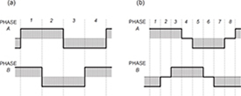
Fig. 6.12. Phase current waveforms: (a) full-stepping, two phases on, (b) half-stepping.

Images

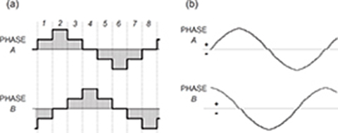
Fig. 6.13. Phase current waveforms to produce approximately equal thrust: (a) half-step current, profiled, (b) microstepping mode.

Approximately equal thrust in every step can be obtained by supplying a higher current when only one phase is energized (Fig. 6.13). The motor will not get overheated because it is designed to operate with two phases to be energized simultaneously. Since the winding losses are proportional to the current squared, approximately the same winding losses are dissipated if two phases are fed at the same time or if only one phase is fed with current increased by 2–√ $\sqrt{2}$ .

The same currents in both two phases produce an intermediate step equal to half of that for only one phase being energized. With unequal two-phase currents, the position of the platen will be shifted toward the stronger pole. This effect is utilized in the microstepping controller that subdivides the basic motor step by proportioning the current in the two-phase winding (Fig. 6.13b). Thus, the step size is reduced, and the operation at low speeds is very smooth. The motor in its microstepping mode operates similar to a two-phase synchronous motor and can even be driven directly from 50 or 60 Hz sinusoidal power supply, provided that a capacitor is connected in series with one phase.

The advantages of microstepping a linear stepping motor include [40]

higher resolution for positioning accuracy,
smoothness at low speeds,
wide speed range,
minimal force loss at resonant frequencies.

6.5.2 Electronic Controllers

To obtain the best performance at minimum settling time (Fig. 6.14), an accelerometer feedback is added, which provides electronic damping to the motor [40]. Accelerometer damping is recommended for HLSM applications that require

very short settling time (Fig. 6.14),
repetitive moves or periodic acceleration transients,
maximum force utilization.

The block diagram of an HLSM controller is shown in Fig. 6.15. Power amplifiers of bipolar type are current controlled and use about 20 kHz fixed frequency and PWM. The resolution is from 50 to 125 microsteps per full step [40].

6.6 Precision Linear Positioning

Linear motors are now playing a key role in advanced precision linear positioning [22]. Linear precision positioning systems can be classified into open-loop systems with HLSMs and closed-loop servo systems with LSMs, LBMs, or LIMs (Fig. 6.16).

Images

Fig. 6.14. HLSM settling time. 1 — with accelerometer, 2 — without accelerometer.

Images

Fig. 6.15. Block diagram of an HLSM controller.

A PM LBM (or LSM) driven positioning stage is shown in Fig. 6.17 [161]. A stationary base is made of aluminum, steel, ceramic, or granite plate. It provides a stable, precise, and flat platform to which all stationary positioning components are attached. The base of the stage is attached to the host system with the aid of mounting screws.

The moving table accommodates all moving positioning components. To achieve maximum acceleration, the mass of the moving table should be as small as possible, and usually aluminum is used as a lightweight material. A number of mounting holes on the moving table is necessary to fix the payload to the mounting table.

Linear bearing rails provide a precise guidance to the moving table. Minimum one bearing rail is required. Linear ball bearing or air bearings are attached to each rail.

The armature of a linear motor is fastened to the moving table and reaction rail (PM excitation system) is built in the base between the rails (Fig. 6.17).

A linear encoder is needed to obtain precise control of position of the table, velocity and acceleration. The readhead of the encoder is attached to the moving table.

Images

Fig. 6.16. Typical linear positioning systems: (a) closed-loop servo system with a.c. or d.c. linear motors, (b) open-loop positioning system with HLSMs, (c) closed-loop positioning system with HLSMs.

Images

Fig. 6.17. Linear positioning stage driven by PM LBM: 1 — base, 2 — moving table, 3 — armature of LBM, 4 — PMs, 5 — linear bearing, 6 — encoder, 7 — cable carrier, 8 — limit switch. Courtesy of Normag, Santa Clarita, CA, USA.

Noncontact limit switches fixed to the base provide an over-travel protection and initial homing. A cable carrier accommodates and routes electrical cables between the moving table and stationary connector box fixed to the base.

An HLSM-driven linear precision stage is of similar construction. Instead of PMs between bearing rails, it has a variable reluctance platen. HLSMs usually need air bearings and, in addition to the electrical cables, an air hose between air bearings and the compressor is required. Comparison between an HLSM and LSM of similar size with air bearings is given in [102].

An enclosed linear positioning stage shown in Fig. 6.18 is equipped with bellows covers (protection against dust and debris), in addition to components sketched in Fig. 6.17 [161].

Images

Fig. 6.18. Enclosed linear positioning stage. 1 — base, 2 — moving table, 3 — bellows cover, 4 — cable carrier, 4 — input/output terminals. Courtesy of Normag, Santa Clarita, CA, USA.

Linear positioning stages with moving coreless armature windings arranged vertically are shown in Fig. 6.19. Fig. 6.19a shows a stage with one moving armature [222], while Fig. 6.19b shows a twin armature stage [16]. A coreless moving armature does not have any ferromagnetic materials so that the positioning stage does not produce any cogging thrust. Moreover, a lightweight moving armature provides high-speed response and high acceleration.

It is possible to employ more than two linear motors in parallel. Fig. 6.20a shows a linear positioning stage with three moving PM excitation systems, while Fig. 6.20b shows a similar construction with four stationary PMs and three moving coreless armature windings [3]. Fig. 6.21 shows a multilayer positioning stage with five moving PM excitation systems [3].

The FEM modeling indicates that the magnetic flux density distribution along the air gap of multilayer LSMs is nonuniform [3]. Any nonuniformity in the magnetic field distribution causes different values of EMFs induced in coils that are distributed along the armature. Consequently, the current density distribution in the armature winding is also nonuniform, which can cause local overheating of the armature system.

Images

Fig. 6.19. Linear positioning stages with moving coreless armature windings: (a) single armature, (b) twin armature. 1 — base, 2 — moving table, 3 — armature of LBM, 4 — PMs, 5 — linear bearing, 6 — linear scale of encoder, 7 — readhead of encoder, 8 — yoke, 9 — cable.

Images

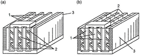
Fig. 6.20. Triple linear positioning stages with moving (a) PMs, (b) coreless armature windings. 1 — coreless armature winding, 2 — PMs, 3 — base. Courtesy of Technical University of Szczecin, Poland, and Institute of Electrodynamics of UNAS, Kiev, Ukraine.

Linear positioning stages are used in semiconductor technology, electronic assembly, quality assurance, laser cutting, optical scanning, water jet cutting, gantry systems (x, y, z stages), color printers, plotters, and Cartesian coordinate robotics [222].

Fig. 6.22 shows an application of a linear positioning stage, according to Fig. 6.19b, to a recorder [16]. The table driven by a twin armature LSM or LBM moves along the rotating drum. The optical recording head fixed to the moving table writes data on the track of the recording film. The mass of recording head is 2 kg, and the width of track is 1.4 mm. The recording head, while writing data, must keep constant position with high accuracy ±1 μm. After writing, the head needs to move quickly to the next track and settle down within 20 ms. The maximum speed and maximum acceleration are 0.22 m/s and 44 m/s², respectively [16].

Images

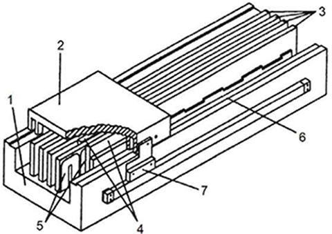
Fig. 6.21. Multilayer linear positioning stage. 1 — base, 2 — moving table, 3 — armature, 4 — PMs, 5 — armature coils, 6 — linear bearing, 7 — readhead of linear encoder. Courtesy of Technical University of Szczecin, Poland, and Institute of Electrodynamics of UNAS, Kiev, Ukraine.

Images

Fig. 6.22. Recorder with a linear positioning stage. 1 — moving table, 2 — base of positioning stage, 3 — recording head, 4 — rotary motor, 5 — recording track, 6 — recording film, 7 — rotary drum, 8 — pedestal. Courtesy of Hitachi Metals Ltd, Saitama, Japan.

Examples

Example 6.1

Given are specifications of a 3-phase, 4-pole, single-sided LSM with surface configuration of PMs and the following specifications: τ = 40 mm, w_M = 36 mm, L_i = 80 mm, B_mg = 0.65 T, N₁ = 440, s₁ = 24, w_c = τ (full-pitch coils, two-layer winding).

Find the EMF and electromagnetic thrust for sine-wave and square-wave control assuming that the rated armature current Ia=Isqa=8.0 A $I_{a} = I_{a}^{s q} = 8.0 A$ and f = 30 Hz for both methods of control, and Ψ = 0 for the sine-wave motor.

Solution

The pole shoe width b_p = w_M = 36 mm, the number of slots per pole Q₁ = 24/8 = 3, the number of slots per pole per phase q₁ = 24/(8 × 3) = 1, the winding factor calculated on the basis of eqns (2.39), (2.40), (2.41) k_d₁ = sin(π/(2 × 3)/[1 × sin(π/(2 × 3 × 1)] = 1, k_p₁ = sin(π × 40/(2 × 40) = 1, k_w₁ = 1 × 1 = 1, pole shoe width to pole pitch ratio according to eqn (3.11) α_i = 36/40 = 0.9, and the synchronous speed v_s = 2×30×0.04 = 2.4 m/s. The number of coils per phase of a two-layer armature winding is N_c = s₁/m₁ = 24/3 = 8, and the number of turns per coil is n_c = N₁/N_c = 440/8 = 55.

Sine-wave motor

Form factor of the excitation field according to eqn (3.10)

k f = 4 π sin (0.9 π 2) = 1.258

$k_{f} = \frac{4}{π} \sin (\frac{0.9 π}{2}) = 1.258$

Amplitude of the fundamental harmonic of magnetic flux density

B m g 1 = k f B m g = 1.258 \times 0.65 = 0.817 T

$B_{m g 1} = k_{f} B_{m g} = 1.258 \times 0.65 = 0.817 T$

Fundamental harmonic of the magnetic flux according to eqn (3.26)

Φ f 1 = 2 π 0.04 \times 0.08 \times 1.258 \times 0.65 = 1.665 \times 10 - 3 Wb

$Φ_{f 1} = \frac{2}{π} 0.04 \times 0.08 \times 1.258 \times 0.65 = 1.665 \times 10^{- 3} Wb$

It is assumed that Φ_f ≈ Φ_f1 = 1.665 × 10⁻³ Wb. Amplitude of the fundamental harmonic of EMF induced in a single conductor of the armature winding

E m f 1 = B m g 1 L i v s = 0.817 \times 0.08 \times 2.4 = 0.157 V

$E_{m f 1} = B_{m g 1} L_{i} v_{s} = 0.817 \times 0.08 \times 2.4 = 0.157 V$

Armature constant c_E according to eqn (6.2)

c E = π 0.04 1 2 - \sqrt 440 \times 1 = 24 435.9 1 / m

$c_{E} = \frac{π}{0.04} \frac{1}{\sqrt{2}} 440 \times 1 = 24 435.9 1 / m$

Armature constant k_E according to eqn (6.3)

k E = 24 435.9 \times 1.665 \times 10 - 3 = 40.691 Vs / m

$k_{E} = 24 435.9 \times 1.665 \times 10^{- 3} = 40.691 Vs / m$

EMF per phase at synchronous speed v_s = 2.4 m/s

E f = 40.691 \times 2.4 = 97.66 V

$E_{f} = 40.691 \times 2.4 = 97.66 V$

The characteristic E_f = f(v_s), neglecting the armature reaction and saturation, is a straight line. For example, at v_s = 1 m/s, E_f = 40.69 V, at v_s = 2 m/s, E_f = 81.38 V, at v_s = 4.8 m/s, E_f = 195.3 V, etc.

Thrust constant c_F according to eqn (6.5)

c F = 2 c E = 2 \times 24 435.9 = 48 871.7 1 / m

$c_{F} = 2 c_{E} = 2 \times 24 435.9 = 48 871.7 1 / m$

Thrust constant k_F according to eqn (6.6)

k F = 48 871.7 \times 1.665 \times 10 - 3 = 81.383 N / A

$k_{F} = 48 871.7 \times 1.665 \times 10^{- 3} = 81.383 N / A$

Electromagnetic thrust at rated current I_a = 8.0 A according to eqn (6.7)

F d x = 3 2 81.383 \times 8.0 = 976.6 N

$F_{d x} = \frac{3}{2} 81.383 \times 8.0 = 976.6 N$

Neglecting armature reaction and saturation, the characteristic F_dx = f(I_a) is also a straight line. For I_a = 2 A, F_dx = 244.15 N, for I_a = 6 A, F_dx = 732.44 N, for I_a = 1.2 × 8.0 A, F_dx = 1172 N, etc.

Square-wave motor

Magnetic flux calculated on the basis of eqn (6.10)

Φ (s q) f = 0.9 \times 0.04 \times 0.08 \times 0.65 = 1.872 \times 10 - 3 Wb

$Φ_{f}^{(s q)} = 0.9 \times 0.04 \times 0.08 \times 0.65 = 1.872 \times 10^{- 3} Wb$

EMF constant c_Edc according to eqn (6.12)

c E d x = 4 0.04 440 \times 1 = 440001 / m

$c_{E d x} = \frac{4}{0.04} 440 \times 1 = 44 000 1 / m$

EMF constant k_Edc according to eqn (6.13)

k E d c = 44000 \times 1.872 \times 10 - 3 = 82.368 Vs / m

$k_{E d c} = 44 000 \times 1.872 \times 10^{- 3} = 82.368 Vs / m$

EMF at synchronous speed v_s = 2.4 m/s

E (s q) f = 44000 \times 2.4 = 197.68 V

$E_{f}^{(s q)} = 44 000 \times 2.4 = 197.68 V$

Please note that the above EMF is induced in two phases connected in series (two phases are conducting at the same time). For sine-wave motor, the EMF E_f = 97.66 is line-to-neutral EMF.

The thrust constants c_{F dc} and k_{F dc} are given by eqn (6.15), i.e.,

c F d c = c E d c = 440001 / m; k F d c = 44000 \times 1.872 \times 10 - 3 = 82.368 N / A

$\begin{matrix} c_{F d c} = c_{E d c} = 44 000 1 / m; & k_{F d c} = 44 000 \times 1.872 \times 10^{- 3} = 82.368 N / A \end{matrix}$

Thrust at rated current I_a = 8 A according to eqn (6.14)

F (s q) d x = 82.368 \times 8.0 = 658.9 N

$F_{d x}^{(s q)} = 82.368 \times 8.0 = 658.9 N$

Square-wave motor to sine-wave motor thrust ratio

F ( s q ) d x F d x = 658.9 976.6 = 0.675

$\frac{F_{d x}^{(s q)}}{F_{d x}} = \frac{658.9}{976.6} = 0.675$

Using eqn (6.17) for Ia=I(sq)a $I_{a} = I_{a}^{(s q)}$

F ( s q ) d x F d x \approx 0.6 1.872 \times 10 - 3 1.665 \times 10 - 3 \approx 0.675

$\frac{F_{d x}^{(s q)}}{F_{d x}} \approx 0.6 \frac{1.872 \times 10^{- 3}}{1.665 \times 10^{- 3}} \approx 0.675$

Example 6.2

For a 2nd order mass-spring-damper system described by eqn (1.26) find the transfer function.

Solution

Eqn (1.26) can be also written as

x ¨ + D v m x ˙ + k s m x = k s m F x ( t ) k

$\ddot{x} + \frac{D_{v}}{m} \dot{x} + \frac{k_{s}}{m} x = \frac{k_{s}}{m} \frac{F_{x} (t)}{k}$

Putting D_v/m = 2ζω_n, k_s/m = ω_n, and F_x(t)/k_s = y(t), the mass-spring-damper system equation can be written in terms of the damping factor ζ and undamped natural frequency ω_n, i.e.,

x ¨ + 2 ζ ω n x ˙ + ω 2 n x = ω 2 n y (t)

$\ddot{x} + 2 ζ ω_{n} \dot{x} + ω_{n}^{2} x = ω_{n}^{2} y (t)$

Transfer functions are defined by the ratio between the Laplace transform of the input, i.e. the normalized force y(t), and the output signal, i.e., the position of the mass x(t). Taking the Laplace transform on both sides of the above equation

L {x ¨ + 2 ζ ω n x ˙ + ω 2 n x} = L {ω n y (t)} s 2 X (s) + 2 ζ ω n s X (s) + ω 2 n X (s) = ω 2 n Y (s) {s 2 + 2 ζ ω n s + ω 2 n} X (s) = ω 2 n Y (s)

$\begin{matrix} L {\ddot{x} + 2 ζ ω_{n} \dot{x} + ω_{n}^{2} x} = L {ω_{n} y (t)} \\ s^{2} X (s) + 2 ζ ω_{n} s X (s) + ω_{n}^{2} X (s) = ω_{n}^{2} Y (s) \\ {s^{2} + 2 ζ ω_{n} s + ω_{n}^{2}} X (s) = ω_{n}^{2} Y (s) \end{matrix}$

the transfer function of the mass-spring-damper system is

T (s) = X ( s ) Y ( s ) = ω 2 n s 2 + 2 ζ ω n s + ω 2 n

$T (s) = \frac{X (s)}{Y (s)} = \frac{ω_{n}^{2}}{s^{2} + 2 ζ ω_{n} s + ω_{n}^{2}}$

The denominator of the transfer function is the same as the characteristic polynomial of eqn (1.26). The roots of the characteristic polynomial are called poles of the transfer function T (s).

Example 6.3

A flat, single-sided, three-phase PM LSM has the following parameters: R₁ = 1.6 Ω, X_sd = 5.0 Ω, X_sq = 4.9 Ω at f = 50 Hz. The axial length of the stack is 0.24 m, number of poles 2p = 8, height of PM h_M = 5 mm, coercivity of PM H_c = 850 kA/m, EMF per phase E_f = 80 V. Find

terminal voltage, input power, electromagnetic power, and electromagnetic thrust at I_ad = −2.0 A and I_aq = 10 A;
terminal voltage, input power, electromagnetic power, and electromagnetic thrust as functions of I_aq for I_a = 10 A = const, ϕ_f = const, and 1.0 ≤ I_aq ≤ 10.0 A.

Assumption: LSM operates at steady-state conditions, i.e., (d/dt)L_sdi_ad = (d/dt)L_sqi_aq = 0.

Solution

(a) Terminal voltage, input power, electromagnetic power, and electromagnetic thrust at I_ad = −2.0 A and I_aq = 10 A

The angular frequency ω = 2π50.0 = 314.16 rad/s, pole pitch τ = 0.24/8 = 0.03 m, linear synchronous speed v_s = 2 × 50.0 × 0.03 = 3.0 m/s, armature currents in dq0 reference frame iad=2–√(−2.0)=−2.828 A,iaq=2–√(10.0)=14.142 A $i_{a d} = \sqrt{2} (- 2.0) = - 2.828 A, i_{a q} = \sqrt{2} (10.0) = 14.142 A$ , fictitious field excitation currents (equivalent MMF) of PM I_f = 0.005 × 850 000 = 4250 A, and if=2–√×4250.0=6010.4 A $i_{f} = \sqrt{2} \times 4250.0 = 6010.4 A$ .

Synchronous inductances in the d- and q-axis

L s d = 5.0 314.16 = 0.0159 H L s q = 4.9 314.16 = 0.0156 H

$\begin{matrix} L_{s d} = \frac{5.0}{314.16} = 0.0159 H & L_{s q} = \frac{4.9}{314.16} = 0.0156 H \end{matrix}$

Rotor linkage flux

$ψ_{f} = \sqrt{2} \frac{80.0}{314.16} = 0.36 Wb$

Armature rms current

$I_{a d} = \sqrt{{(- 2.0)}^{2} + 10^{2}} = 10.2 A$

Angle between armature current and q-axis

$Ψ = arccos (\frac{I_{a q}}{I_{a}}) = arccos (\frac{10}{10.2}) = {11.21}^{\circ}$

Voltages v_1d and v_1q in the d-q reference frame for steady-state conditions are calculated with the aid of eqn (6.31), in which (d/dt)L_sdi_ad = (d/dt)L_sqi_aq = 0, i.e.,

$\begin{matrix} [\begin{matrix} v_{1 d} \\ v_{1 q} \end{matrix}] = [\begin{matrix} R_{1} & - X_{s q} \\ X_{s d} & R_{1} \end{matrix}] [\begin{matrix} i_{a d} \\ i_{a q} \end{matrix}] + [\begin{matrix} 0 \\ ω ψ_{f} \end{matrix}] \\ = [\begin{matrix} 1.6 & - 4.9 \\ 5.0 & 1.6 \end{matrix}] [\begin{matrix} - 2.828 \\ 14.142 \end{matrix}] + [\begin{matrix} 0 \\ 314.16 \times 0.36 \end{matrix}] = [\begin{matrix} - 73.82 \\ 121.62 \end{matrix}] \end{matrix}$

In phasor form with the d-q reference frame $V_{1 d} = - 73.82 / \sqrt{2} = - 52.2 V, V_{1 q} = 121.62 / \sqrt{2} = 86.0 V$ , and the rms phase voltage $V_{1} = \sqrt{{(- 52.2)}^{2} + {86.0}^{2}} = 100.6 V$ . Input power according to eqn (6.32)

$p_{i n} = \frac{3}{2} [(- 73.82) \times (- 2.828) + 86.0 \times 14.142] = 2893 W$

Electromagnetic power according to eqn (6.34)

$p e l m = \frac{3}{2} \times 314.16 [0.36 + (0.0159 - 0.0156) (- 2.828)] \times 14.142 = 2394 W$

Electromagnetic thrust developed by the LSM is calculated on the basis of eqn (6.35), i.e.,

$F_{d x} = \frac{2394}{3.0} = 798 N$

(b) Terminal voltage, input power, electromagnetic power, and electromagnetic thrust as functions of I_aq for I_a = 10 A = const and 1.0 ≤ I_aq ≤ 10.0 A

The d-axis current in phasor form as a function of I_aq

$I_{a d} (I_{a q}) = \sqrt{I_{a}^{2} - I_{a q}^{2}}$

$i_{a d} (I_{a q}) = \sqrt{2} I_{a d} (I_{a q})$

The voltages in the d- and q-axis are calculated with the aid of eqn (6.31), i.e.,

$\begin{matrix} v_{1 d} (I_{a q}) = R_{1} i_{a d} (I_{a q}) - X_{s q} \sqrt{2} I_{a q} \\ v_{1 q} (I_{a q}) = X_{s d} i_{a d} (I_{a q}) + R_{1} \sqrt{2} I_{a q} + ω ψ_{f} \end{matrix}$

Armature rms voltage

$V_{1} (I_{a q}) = \frac{1}{\sqrt{2}} \sqrt{{[v_{1 d} (I_{a q})]}^{2} + {[v_{1 q} (I_{a q})]}^{2}}$

Table 6.1. Voltage, angle Ψ, input power, electromagnetic power, and thrust as functions of I_aq at I_a = const and ϕ_f = const. Example 6.2

Images

Input power according to eqn (6.32)

$p_{i n} (I_{a q}) = \frac{3}{2} [v_{1 d} (I_{a q}) i_{a d} (I_{a q}) + v_{1 q} (I_{a q}) \sqrt{2} I_{a q}]$

Electromagnetic power according to eqn (6.34)

$p_{e l m} = \frac{3}{2} ω [ψ_{f} + (L_{s q} - L_{s q}) i_{a d} (I_{a q})] \sqrt{2} I_{a q}$

Angle between the current I_a and q axis

$Ψ (I_{a q}) = arccos (\frac{I_{a q}}{I_{a}})$

Electromagnetic thrust developed by the LSM is calculated on the basis of eqn (6.35), i.e.,

$F_{d x} (I_{a q}) = \frac{p_{e l m} (I_{a q})}{υ_{s}}$

The results of the calculations are listed in Table 6.1.

Example 6.4

For f = 60 Hz, t = 0.006 s, rms currents I_aA = I_aB = I_aC = 10 A, and rms voltages V_1A = V_1B = V_1C = 230 V, find the dq0 components of currents and voltages. Prove that the product of transformation matrices [B][B]⁻¹ = [I], where [I] is the square identity matrix. Calculate the power in ABC and dq0 reference frames. The phase angle between the current and voltage is 30°.

Solution

Angular frequency

$ω = 2 π f = 2 π 60 = 376.99 rad / s$

The angle Θ between A-phase and d-axis

$Θ = ω t = 376.99 \times 0.006 = 0.262 rad = {129.6}^{\circ}$

Phase instantaneous currents

$\begin{matrix} i_{a A} = \sqrt{2} \times 10 \cos ({129.6}^{\circ} - 30^{\circ}) = - 2.358 A \\ i_{a B} = \sqrt{2} \times 10 \cos ({129.6}^{\circ} - 120^{\circ} - 30^{\circ}) = 13.255 A \\ i_{a C} = \sqrt{2} \times 10 \cos ({129.6}^{\circ} + 120^{\circ} - 30^{\circ}) = - 10.897 A \end{matrix}$

Phase instantaneous voltages

$\begin{matrix} υ_{1 A} = \sqrt{2} \times 230 \cos ({129.6}^{\circ}) = - 207.334 A \\ υ_{1 B} = \sqrt{2} \times 230 \cos ({129.6}^{\circ} - 120^{\circ}) = 320.714 V \\ υ_{a C} = \sqrt{2} \times 230 \cos ({129.6}^{\circ} + 120^{\circ}) = - 113.38 V \end{matrix}$

Blondel transformation matrix given by eqn (6.41)

$[B] = \frac{2}{3} [\begin{matrix} \cos (Θ) & \cos (Θ - \frac{2 π}{3}) & \cos (Θ + \frac{2 π}{3}) \\ - \sin (Θ) & - \sin (Θ - \frac{2 π}{3}) & - \sin (Θ + \frac{2 π}{3}) \\ \frac{1}{2} & \frac{1}{2} & \frac{1}{2} \end{matrix}] = [\begin{matrix} - 0.425 & 0.657 & - 0.232 \\ - 0.514 & - 0.111 & 0.625 \\ 0.333 & 0.333 & 0.333 \end{matrix}]$

Inverse of matrix [B] according to eqn (6.43)

${[B]}^{- 1} = [\begin{matrix} \cos (Θ) & - \sin (Θ) & 1 \\ \cos (Θ - \frac{2 π}{3}) & - \sin (Θ - \frac{2 π}{3}) & 1 \\ \cos (Θ + \frac{2 π}{3}) & - \sin (Θ + \frac{2 π}{3}) & 1 \end{matrix}] = [\begin{matrix} - 0.637 & - 0.771 & 1 \\ 0.986 & - 0.167 & 1 \\ - 0.349 & 0.937 & 1 \end{matrix}]$

Matrix [B] multiplied by matrix [B]⁻¹ must give a square diagonal identity matrix, i.e.,

$[B] {[B]}^{- 1} = [\begin{matrix} - 0.425 & 0.657 & - 0.232 \\ - 0.514 & - 0.111 & 0.625 \\ 0.333 & 0.333 & 0.333 \end{matrix}] = [\begin{matrix} - 0.637 & - 0.771 & 1 \\ 0.986 & - 0.167 & 1 \\ - 0.349 & 0.937 & 1 \end{matrix}] = [\begin{matrix} 1 & 0 & 0 \\ 0 & 1 & 0 \\ 0 & 0 & 1 \end{matrix}]$

Currents in dq0 reference frame

$[\begin{matrix} i_{a d} \\ i_{a q} \\ i_{0} \end{matrix}] = [B] = [\begin{matrix} i_{a A} \\ i_{a B} \\ i_{a C} \end{matrix}] = [\begin{matrix} - 0.425 & 0.657 & - 0.232 \\ - 0.514 & - 0.111 & 0.625 \\ 0.333 & 0.333 & 0.333 \end{matrix}] = [\begin{matrix} - 2.358 \\ 13.255 \\ - 10.897 \end{matrix}] = [\begin{matrix} 12.247 \\ - 7.071 \\ 0.0 \end{matrix}]$

Voltages in dq0 reference frame

$[\begin{matrix} υ_{1 d} \\ υ_{1 q} \\ υ_{0} \end{matrix}] = [B] = [\begin{matrix} υ_{1 A} \\ υ_{1 B} \\ υ_{1 C} \end{matrix}] = [\begin{matrix} 0.425 & 0.657 & - 0.232 \\ - 0.514 & - 0.111 & 0.625 \\ 0.333 & 0.333 & 0.333 \end{matrix}] = [\begin{matrix} - 207.334 \\ 320.714 \\ - 113.38 \end{matrix}] = [\begin{matrix} 325.269 \\ 0.0 \\ 0.0 \end{matrix}]$

If ABC current and voltage systems are balanced, the currents and voltages in dq0 reference frame are independent of time.

Transformation from dq0 to ABC frame will confirm the correctness of calculations, i.e.,

$[\begin{matrix} i_{a A} \\ i_{a B} \\ i_{a C} \end{matrix}] = {[B]}^{- 1} = [\begin{matrix} i_{a d} \\ i_{a q} \\ i_{0} \end{matrix}] = [\begin{matrix} - 0.637 & - 0.771 & 1 \\ 0.986 & - 0.167 & 1 \\ - 0.349 & 0.937 & 1 \end{matrix}] = [\begin{matrix} 12.247 \\ - 7.071 \\ 0.0 \end{matrix}] = [\begin{matrix} - 2.358 \\ 13.255 \\ - 10.897 \end{matrix}]$

$[\begin{matrix} υ_{1 A} \\ υ_{1 B} \\ υ_{1 C} \end{matrix}] = {[B]}^{- 1} = [\begin{matrix} υ_{1 d} \\ υ_{1 q} \\ υ_{0} \end{matrix}] = [\begin{matrix} - 0.637 & - 0.771 & 1 \\ 0.986 & - 0.167 & 1 \\ - 0.349 & 0.937 & 1 \end{matrix}] = [\begin{matrix} 325.269 \\ 0 \\ 0 \end{matrix}] = [\begin{matrix} - 207.334 \\ 320.714 \\ - 113.38 \end{matrix}]$

The power on the basis of eqn (6.45)

$p_{i n} (- 207.334) \times (- 2.358) + 320.714 \times 13.255 + (- 113.38) \times (- 10.897) = 5975.57 VA$

The power on the basis of eqn (6.46)

$p_{i n} = \frac{3}{2} [325.269 \times 12.247 + 0.0 \times (- 7.071) + 2 \times 0.0 \times 0.0] = 5975.57 VA$

Both equations give the same results. For balanced current and voltage systems in ABC reference frame, the power is independent of time.

^¹In medicine, a synapse is a point at which a nerve charge passes from one basic reaction unit cell to another.

^²The product [A][A]⁻¹ = [I], where [A]⁻¹ is the inverse matrix and [I] is the square identity matrix. The identity matrix is a diagonal stretch of 1s going from the upper-left-hand corner to the lower right, with all other elements being 0.

^³The transpose [A]^T of matrix [A] is formed by interchanging elements a_ij with elements a_ji.

..................Content has been hidden....................

You can't read the all page of ebook, please click here login for view all page.

Table of Contents for
6 Motion Control

6

Motion Control

6.1 Control of AC Motors

6.2 EMF and Thrust of PM Synchronous and Brushless Motors

6.2.1 Sine-Wave Motors

6.2.2 Square-Wave (Trapezoidal) Motors

6.3 Model of PM Motor in dq Reference Frame

6.4 Thrust and Speed Control of PM Motors

6.4.1 Open Loop Control

6.4.2 Closed Loop Control

6.4.3 Zero Direct-Axis Current Control

6.4.4 Flux-Weakening Control

6.4.5 Direct Thrust Control

6.4.6 Fuzzy Control

6.5 Control of Hybrid Stepping Motors

6.5.1 Microstepping

6.5.2 Electronic Controllers

6.6 Precision Linear Positioning

Examples

Table of Contents for 6 Motion Control

Create new playlist

Sign In

Sign Up

Table of Contents for
6 Motion Control