2 Materials and Construction

Search in book...
Toggle Font Controls
Create new playlist

Name your new playlist

Playlist description (optional)
Sign In

Email address

Password

Forgot Password?

or

Continue with Facebook

Continue with Google
Sign Up

Full Name

Email address

Confirm Email Address

Password

or

Continue with Facebook

Continue with Google

All materials used in the construction of electrical machines can be divided into three groups:

Active materials, i.e., electric conductors (magnet wires), superconductors, electrical steels, sintered powders and PMs
Insulating materials
Construction materials

All current conducting materials (with high electric conductivity), magnetic flux conducting materials (with high magnetic permeability), and PMs are called active materials. They serve in the excitation of the EMF and MMF, concentrate the magnetic flux in the desired place or direction, and help to maximize the electromagnetic forces. Ferromagnetic materials are divided into soft ferromagnetic materials, i.e., with a narrow hysteresis loop, and hard ferromagnetic materials or PMs, i.e., with a wide hysteresis loop.

Insulating materials isolate electrically the current-carrying conductors from the other parts of electrical machines.

There are no insulating materials for the magnetic flux. Leakage fluxes can only be reduced by a proper shaping of the magnetic circuit or using electromagnetic or electrodynamic screens (shielding).

Construction materials are necessary for structural purposes intended for the transmission and withstanding of mechanical loads and stresses. In the electrical machine industry, mild carbon steel, alloyed steel, cast iron, wrought iron, non-ferromagnetic steel, nonferromagnetic metals and their alloys, and plastic materials are used as construction materials.

2.2 Laminated Ferromagnetic Cores

From the electromagnetic point of view, laminated ferromagnetic cores are used to improve the propagation of electromagnetic waves in conductive ferromagnetic materials. In thin ferromagnetic sheets, i.e., with their thicknesses below 1 mm, the skin effect at power frequencies 50 to 60 Hz practically does not exist. Since in laminated cores eddy currents are reduced, the damping effect of the electromagnetic field by eddy currents is reduced, too. The alternating magnetic flux occurs in the whole sheet cross section, and its distribution is practically uniform inside the laminated stack. Considering the skin effect, stacking factor, hysteresis losses, eddy-current losses, reactive power (magnetizing current), and easy stamping, the best thickness is 0.5 to 0.6 mm for 50-Hz electrical machines, and 0.2 to 0.35 mm for 400-Hz electrical machines [226].

The main losses in a ferromagnetic core with its mass m_{F e} at any fre quency f and given magnetic flux density B are calculated as

Δ P F e = k F e Δ p 1 / 50 (f 50) 4 / 3 B 2 m F e (2.1)

$Δ P_{F e} = k_{F e} Δ p_{1 / 50} {(\frac{f}{50})}^{4 / 3} B^{2} m_{F e} (2.1)$

where kFe>1 $k_{F_{e}} > 1$ is the coefffcient for including the difference in the distribution of the magnetic field in the core and in the sample in which the specific core losses have been measured, and for including the losses due to rotational magnetic reversal and the “work hardening” during stamping; Δp_1/50 is the specific core loss at f = 50 Hz and B = 1 T; f is the frequency of the magnetic field; and B is the magnetic flux density.

Better results are obtained if the losses are divided into hysteresis lossess and eddy-current losses, i.e.,

Δ P F e = Δ P h + Δ P e = [k h c h (f 50) B 2 + k e c e (f 50) 2 B 2] m F e (2.2)

$Δ P_{F e} = Δ P_{h} + Δ P_{e} = [k_{h} c_{h} (\frac{f}{50}) B^{2} + k_{e} c_{e} {(\frac{f}{50})}^{2} B^{2}] m_{F e} (2.2)$

where k_h = 1 to 2, k_e = 2 to 3, c_h = 2 to 5 Ws/(T²kg) is the hysteresis constant, and c_e = 0.5 to 23 Ws²/(T²kg) is the eddy-current constant. The thicker the sheet, the higher the constants c_h and c_e. Eqn (2.2) can only be used if accurate values of c_h and c_e are known. In most cases the constants c_h and c_e are not specified.

The armature core losses ΔPFe $Δ P_{F_{e}}$ can be calculated on the basis of the specific core losses and masses of teeth and yoke, i.e.,

Δ P F e = Δ p 1 / 50 (f 50) 4 / 3 [k a d t B 2 t m t + k a d c B 2 c m c] (2.3)

$Δ P_{F e} = Δ p_{1 / 50} {(\frac{f}{50})}^{4 / 3} [k_{a d t} B_{t}^{2} m_{t} + k_{a d c} B_{c}^{2} m_{c}] (2.3)$

where k_adt > 1 and k_ady > 1 are the factors accounting for the increase in losses due to metallurgical and manufacturing processes, Δp_1/50 is the specific core loss in W/kg at 1 T and 50 Hz, B_t is the magnetic flux density in a tooth, B_c is the magnetic flux density in the core (yoke), m_t is the mass of the teeth, and m_c is the mass of the core. For the teeth, k_adt = 1.7 to 2.0, and for the core, k_adc = 2.4 to 4.0 [113].

The external surfaces of electrotechnical steel sheets are covered with a thin layer of ceramic materials or oxides to electrically insulate the adjacent laminations in a stack. This insulation limits the eddy currents induced in the core due to a.c. magnetic fluxes. The thickness of the insulation is expressed with the aid of the stacking factor (insulation factor):

k i = \sum n i - - 1 d i \sum n i = 1 ( d i + 2 Δ i ) < 1 (2.4)

$k_{i} = \frac{\sum_{i - - 1}^{n} d_{i}}{\sum_{i = 1}^{n} (d_{i} + 2 Δ_{i})} < 1 (2.4)$

where d_i is the thickness of the ith lamination, and Δ_i is the thickness of the insulation layer of the ith lamination measured on one side. For the stack consisting of laminations of equal thickness d with the thickness of the insulation layer Δ (one side), the stacking factor is

k i = d d + 2 Δ (2.5)

$k_{i} = \frac{d}{d + 2 Δ} (2.5)$

For cold-rolled electrical steel sheets, the stacking factor is k_i = 0.95 to 0.98; for hot-rolled sheets this factor is smaller.

2.2.1 Electrical Sheet-Steels

Typical magnetic circuits of electrical machines and electromagnetic devices are laminated and are mainly made of cold-rolled electrotechnical steel sheets, i.e.,

oriented (anisotropic) textured,
nonoriented with silicon content,
nonoriented without silicon.

Nowadays, hot-rolled electrotechnical steel sheets are almost never used. Elec-trotechnical steel sheets have crystal structure. Oriented steel sheets are used for the ferromagnetic cores of transformers, transducers, and large synchronous generators. Nonoriented steel sheets are used for construction of large, medium, and low-power rotary electrical machines, micromachines, small transformers and reactors, electromagnets, and magnetic amplifiers. Addition of 0.5% to 3.25% of silicon (Si) increases the maximum magnetic permeability corresponding to the critical magnetic field intensity, reduces the area of the hysteresis loop, increases the resistivity (reduces eddy current losses), and practically excludes ageing (increase in the steel losses with time). Thus, owing to the silicon content, the specific core losses are substantially reduced. On the other hand, silicon reduces somewhat permeability in strong fields (saturation magnetic flux density), increases hardness of laminations and, as a consequence, shortens the life of stamping tooling (fast wear of the punching die).

Images

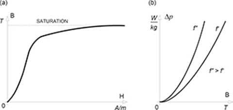
Fig. 2.1. Typical characteristics of electrotechnical steel sheets: (a) magnetization curve B-H, (b) specific core loss curves Δp-B at f = const.

The increase of power loss with time or ageing is caused by an excessive carbon content in the steel. Modern non-oriented fully processed electrical steels are free from magnetic ageing [203].

Fig. 2.1 shows a typical magnetization curve B-H and specific core loss curve Δp-B of electrotechnical steel sheets. The B-H curves are obtained by increasing the magnetic field intensity H from zero in a virgin sample (never magnetized before) as a set of top points of hysteresis loops. Specific core loss curves Δp-B are measured with the aid of Epstein’s apparatus. The shape of the Δp-B curve such as that in Fig. 2.1b is only valid for steel sheets with crystal structure.

Silicon steels are generally specified and selected on the basis of allowable specific core losses (W/kg or W/lb). The most universally accepted grading of electrical steels by core losses is the American Iron and Steel Industry (AISI) system (Table 2.1), the so called “M-grading”. The M number, e.g., M19, M27, M36, etc., indicates maximum specific core losses in W/lb at 1.5 T and 50 or 60 Hz, e.g., M19 grade specifies that losses shall be below 1.9 W/lb at 1.5 T and 60 Hz. Electrical steel M19 offers nearly the lowest core loss in this class of material and is probably the most common grade for motion control products (Fig. 2.2). The specific core loss curve of electrical steel M19 at 50 Hz is plotted in Fig. 2.3.

Nonoriented electrical steels are Fe-Si alloys with random orientation of crystal cubes and practically the same properties in any direction in the plane of the sheet or ribbon. Nonoriented electrical steels are available as both fully processed and semiprocessed products. Fully processed steels are annealed to optimum properties by the manufacturer and ready for use without any additional processing. Semiprocessed steels always require annealing after stamping to remove excess carbon and relieve stress. Better grades of silicon steel are always supplied fully processed, while semiprocessed silicon steel is available only in grades M43 and worse. In some cases, users prefer to develop the final magnetic quality and gain relief from fabricating stresses in laminations or assembled cores for small machines.

Images

Fig. 2.2. Magnetization curve of fully processed Armco DI-MAX nonoriented electrical steel M19.

Images

Fig. 2.3. Specific core loss curve of fully processed Armco DI-MAX nonoriented electrical steel M19 at 50 Hz.

Table 2.1. Silicon-steel designations specified by European, American, Japanese, and Russian standards

Images

The magnetization curve of nonoriented electrical steels M27, M36 and M43 is shown in Fig. 2.4. Core loss curves of nonoriented electrical steels M27, M36 and M43 measured at 60 Hz are given in Table 2.2. Core losses at 50 Hz are approximately 0.79 times the core loss at 60 Hz.

Table 2.3 contains magnetization curves B-H and specific core loss curves Δp-B of three types of cold-rolled, nonoriented electrotechnical steel sheets, i.e., Dk66, thickness d = 0.5 mm, k_i = 0.96, 7740 kg/m³ (Surahammars Bruk AB, Sweden), H-9, d = 0.35 mm, k_i = 0.96, 7650 kg/m³ (Nippon Steel Corporation, Japan) and DI-MAX EST20, d = 0.2 mm, k_i = 0.94, 7650 kg/m³ (Terni–Armco, Italy).

For modern high-efficiency, high-performance applications, there is a need for operating a.c. devices at higher frequencies, i.e., 400 Hz to 10 kHz. Because of the thickness of the standard silicon ferromagnetic steels 0.25 mm (0.010”) or more, core loss due to eddy currents is excessive. Nonoriented electrical steels with thin gauges (down to 0.025 mm thick) for ferromagnetic cores of high-frequency rotating machinery and other power devices are manufactured, e.g., by Arnold Magnetic Technologies Corporation, Rochester, NY, USA. Arnold has two standard nonoriented lamination products: Arnon™ 5 (Figs 2.5 and 2.6) and Arnon™ 7. At frequencies above 400 Hz, they typically have less than half the core loss of standard-gauge nonoriented silicon steel laminations.

Images

Fig. 2.4. Magnetization curve of fully processed Armco DI-MAX nonoriented electrical steels M27, M36, and M43. Magnetization curves for all these three grades are practically the same.

Table 2.2. Specific core losses of Armco DI-MAX nonoriented electrical steels M27, M36, and M43 at 60 Hz

Images

Table 2.3. Magnetization and specific core loss characteristics of three types of cold-rolled, nonoriented electrotechnical steel sheets, i.e., Dk66, thickness 0.5 mm, k_i = 0.96 (Sweden); H-9, thickness 0.35 mm, k_i = 0.96 (Japan); and DI-MAX EST20, thickness 0.2 mm, k_i = 0.94, (Italy).

Images

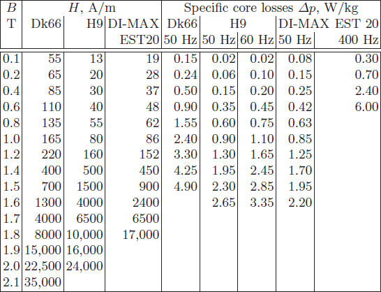
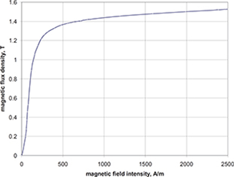
Fig. 2.5. Magnetization curve of Arnon™ 5 nonoriented electrical steel.

Images

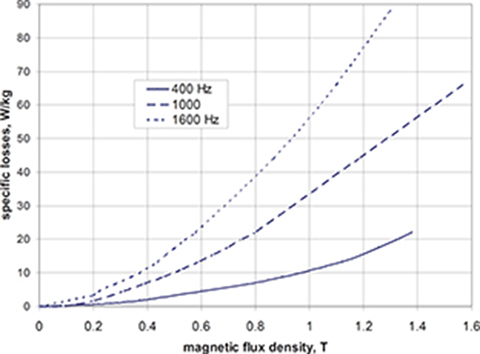
Fig. 2.6. Specific core loss curves of Arnon™ 5 nonoriented electrical steel.

2.2.2 High-Saturation Ferromagnetic Alloys

Cobalt—iron alloys with Co content ranging from 15% to 50% have the highest known saturation magnetic flux density about 2.4 T at room temperature. They are the natural choice for applications where mass and space saving are of prime importance. Additionally, the iron—cobalt alloys have the highest Curie temperatures of any alloy family and have found use in elevated temperature applications. The nominal composition, e.g., for Hiperco 50 from Carpenter, PA, USA is 49% Fe, 48.75% Co, 1.9% V, 0.05% Mn, 0.05% Nb, and 0.05% Si.

The specific mass density of Hiperco 50 is 8120 kg/m³, modulus of elasticity 207 GPa, electric conductivity 2.5 × 10⁶ S/m, thermal conductivity 29.8 W/(m K), Curie temperature 940⁰C, specific core loss about 76 W/kg at 2 T and 400 Hz, and thickness from 0.15 to 0.36 mm. The magnetization curve of Hiperco 50 is shown in Fig. 2.7. Specific losses (W/kg) in 0.356 mm strip at 400 Hz of iron—cobalt alloys from Carpenter are given in Table 2.4.

Images

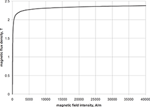
Fig. 2.7. Magnetization curve of Hiperco 50.

Table 2.4. Specific losses (W/kg) in 0.356 mm iron—cobalt alloy strips at 400 Hz.

Images

2.2.3 Permalloys

Small electrical machines and micromachines working in humid or chemical-active atmospheres must have stainless ferromagnetic cores. The best corrosion-resistant ferromagnetic material is permalloy (NiFeMn), but on the other hand, its saturation magnetic flux density is lower than that of electrotech-nical steel sheets. Permalloy is also a good ferromagnetic material for cores of small transformers used in electronic devices and in electromagnetic A/D converters, where a rectangular hysteresis loop is required.

2.2.4 Amorphous Materials

Core losses can be substantially reduced by replacing standard electrotechnical steels with amorphous magnetic alloys. Amorphous ferromagnetic sheets, in comparison with electrical sheets with crystal structure, do not have arranged– in–order, regular inner crystal structure (lattice). Table 2.5 shows physical properties, and Table 2.6 shows specific core loss characteristics of commercially available iron-based METGLAS®¹ amorphous ribbons 2605C0 and 2605SA2 [143].

Table 2.5. Physical properties of iron based METGLAS® amorphous alloy ribbons (AlliedSignals, Inc., Morristown, NJ, USA)

Images

METGLAS amorphous alloy ribbons are produced by rapid solidification of molten metals at cooling rates of about 10^{6 0}C/s. The alloys solidify before the atoms have a chance to segregate or crystallize. The result is a metal alloy with a glass-like structure, i.e., a noncrystalline frozen liquid. METGLAS alloys for electromagnetic applications are based on alloys of iron, nickel, and cobalt. Iron based alloys combine high saturation magnetic flux density with low core losses and economical price. Annealing can be used to alter magne-tostriction to develop hysteresis loops ranging from flat to square.

Table 2.6. Specific core losses of iron based METGLAS® amorphous alloy ribbons (AlliedSignals, Inc., Morristown, NJ, USA).

Images

Owing to very low specific core losses, amorphous alloys are ideal for power and distribution transformers, transducers, and high-frequency apparatus. Application to the mass production of motors is limited by hardness, up to 1100 in Vicker’s scale. Standard cutting methods as a guillotine or blank die are not suitable. The mechanically stressed amorphous material cracks. Laser and EDM cutting methods melt the amorphous material and cause undesirable crystallization. In addition, these methods make electrical contacts between laminations, which contribute to the increased eddy-current and additional losses. General Electric cut amorphous materials in the early 1980s using chemical methods, but these methods were very slow and expensive [148]. Recently, the problem of cutting hard amorphous ribbons has been overcome by using a liquid jet [194]. This method makes it possible to cut amorphous materials in ambient temperature without cracking, melting, crystallization, and electric contacts between isolated ribbons. The face of the cut is very smooth. It is possible to cut amorphous materials on profiles that are suitable for manufacturing laminations for rotary machines, linear machines, chokes, and any other electromagnetic apparatus.

2.2.5 Solid Ferromagnetic Materials

Solid ferromagnetic materials, as cast steel and cast iron are used for salient poles, pole shoes, solid rotors of special induction motors, and reaction rails (platens) of linear motors. Table 2.7 shows magnetization characteristics B-H of a mild carbon steel (0.27% C) and cast iron. Fig. 2.8 shows B-H curves for three types of solid steels: Steel 35 (Poland), Steel 4340 (U.S.), and FeNiCo-MoTiAl alloy (U.S.).

Electrical conductivities of carbon steels are from 4.5 × 10⁶ to 7.0 × 10⁶ S/m at 20⁰C.

Table 2.7. Magnetization curves of solid ferromagnetic materials: 1 — carbon steel (0.27%C), 2 — cast iron.

Images

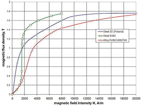
Fig. 2.8. Magnetization curves of solid steels.

Table 2.8. Magnetization and specific core loss characteristics of nonsintered Ac-cucore, TSC Ferrite International, Wadsworth, IL, USA

Images

2.2.6 Soft Magnetic Powder Composites

Powder metallurgy is used in the production of ferromagnetic cores of small electrical machines or ferromagnetic cores with complicated shapes. The components of soft magnetic powder composites are iron powder, dielectric (epoxy resin), and filler (glass or carbon fibers) for mechanical strengthening. Powder composites can be divided into [235]

dielectromagnetics and magnetodielectrics,
magnetic sinters.

Dielectromagnetics and magnetodielectrics are names referring to materials consisting of the same basic components: ferromagnetic (mostly iron powder) and dielectric (mostly epoxy resin) material [235]. The main tasks of the dielectric material are insulation and binding of ferromagnetic particles. In practice, composites containing up to 2% (of their mass) of dielectric materials are considered as dielectromagnetics. Those of higher content of dielectric material are considered as magnetodielectrics [235].

Magnetics International, Inc., Burns Harbor, IN, USA, has developed a new soft powder material, Accucore, which is competitive to traditional steel laminations [1]. The magnetization curve and specific core loss curves of the nonsintered Accucore are given in Table 2.8. When sintered, Accucore has higher saturation magnetic flux density than nonsintered material. The specific density is 7550 to 7700 kg/m³.

2.3 Permanent Magnets

2.3.1 Demagnetization Curve

A permanent magnet (PM) can produce magnetic flux in an air gap with no exciting winding and no dissipation of electric power. As any other ferromagnetic material, a PM can be described by its B-H hysteresis loop. PMs are also called hard magnetic materials, which mean ferromagnetic materials with a wide hysteresis loop.

The basis for the evaluation of a PM is the portion of its hysteresis loop located in the upper left-hand quadrant, called the demagnetization curve (Fig. 2.9). If a reverse magnetic field intensity is applied to a previously magnetized, say, toroidal specimen, the magnetic flux density drops down to the magnitude determined by the point K. When the reverse magnetic flux density is removed, the flux density returns to the point L according to a minor hysteresis loop. Thus, the application of a reverse field has reduced the remanence, or remanent magnetism. Reapplying a magnetic field intensity will again reduce the flux density, completing the minor hysteresis loop by returning the core to approximately the same value of flux density at the point K as before. The minor hysteresis loop may usually be replaced with little error by a straight line called the recoil line. This line has a slope called the recoil permeability μ_rec.

As long as the negative value of applied magnetic field intensity does not exceed the maximum value corresponding to the point K, the PM may be regarded as being reasonably permanent. If, however, a greater negative field intensity H is applied, the magnetic flux density will be reduced to a value lower than that at point K. On the removal of H, a new and lower recoil line will be established.

The general relationship between the magnetic flux density B, intrinsic magnetization B_in = μ₀M due to the presence of ferromagnetic material, and magnetic field intensity H may be expressed as [133, 166]

B = μ 0 H + B i n = μ 0 (H + M) = μ 0 (1 + χ) H = μ 0 μ r H (2.6)

$B = μ_{0} H + B_{i n} = μ_{0} (H + M) = μ_{0} (1 + χ) H = μ_{0} μ_{r} H (2.6)$

in which B, H, B_in, and M are parallel or antiparallel vectors, so that eqn (2.6) can be written in a scalar form. The magnetic permeability of free space μ₀ = 0.4π × 10⁻⁶ H/m. The relative magnetic permeability of ferromagnetic materials μ_r = 1+ξ >> 1. The magnetization vector M = ξH is proportional to the magnetic susceptibility ξ of the material. The flux density μ₀H would be present within, say, a toroid if the ferromagnetic core were not in place. The flux density B_in is the contribution of the ferromagnetic core. The intrinsic magnetization from eqn (2.6) is B_in = B − μ₀H.

Images

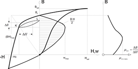
Fig. 2.9. Demagnetization curve, recoil loop, energy of a PM, and recoil magnetic permeability.

A PM is inherently different from an electromagnet. If an external field H_a is applied to the PM, as was necessary to obtain the hysteresis loop of Fig. 2.9, the resultant magnetic field is

H = H a + H d (2.7)

$H = H_{a} + H_{d} (2.7)$

where −H_d is a potential existing between the poles, 180⁰ opposed to B_in, proportional to the intrinsic magnetization B_in. In a closed magnetic circuit, e.g., toroidal circuit, the magnetic field intensity resulting from the intrinsic magnetization H_d = 0. If the PM is removed from the magnetic circuit,

H d = - M b B i n μ o (2.8)

$H_{d} = - \frac{M_{b} B_{i n}}{μ_{o}} (2.8)$

where M_b is the coefficient of demagnetization dependent on the geometry of a specimen. Usually M_b < 1 (see Appendix B).

2.3.2 Magnetic Parameters

PMs are characterized by the following parameters.

Remanent magnetic flux density B_r, or remanence, is the magnetic flux density corresponding to zero magnetic field intensity.

Coercive field strength H_c, or coercivity, is the value of demagnetizing field intensity necessary to bring the magnetic flux density to zero in a material previously magnetized.

Saturation magnetic flux density B_sat corresponds to high values of the magnetic field intensity when an increase in the applied magnetic field produces no further effect on the magnetic flux density. In the saturation region the alignment of all the magnetic moments of domains is in the direction of the external applied magnetic field.

Recoil magnetic permeability μ_rec is the ratio of the magnetic flux density to magnetic field intensity at any point on the demagnetization curve, i.e.,

μ r e c = μ 0 μ r r e c = Δ B Δ H (2.9)

$μ_{r e c} = μ_{0} μ_{r r e c} = \frac{Δ B}{Δ H} (2.9)$

where the relative recoil permeability μ_rrec = 1 to 3.5.

Maximum magnetic energy per unit produced by a PM in the external space is equal to the maximum magnetic energy density per volume, i.e.,

w max = ( B H ) max 2 J / m 3 (2.10)

$\begin{matrix} w_{max} = \frac{{(B H)}_{\max}}{2} & J / m^{3} \end{matrix} (2.10)$

where the product (BH)_max corresponds to the maximum energy density point on the demagnetization curve with coordinates B_max and H_max (Fig. 2.9).

Form factor of the demagnetization curve characterizes the concave shape of the demagnetization curve, i.e.,

γ = ( B H ) max B r H c = B max H max B r H c (2.11)

$γ = \frac{{(B H)}_{max}}{B_{r} H_{c}} = \frac{B_{max} H_{max}}{B_{r} H_{c}} (2.11)$

For a square demagnetization curve γ = 1 and for a straight line (rare-earth PM) γ = 0.25.

Owing to the leakage fluxes, PMs used in electrical machines are subject to nonuniform demagnetization. Therefore, the demagnetization curve is not the same for the whole volume of a PM. To simplify the calculation, in general, it is assumed that the whole volume of a PM is described by one demagnetization curve with B_r and H_c about 5% to 10% lower than those for uniform magnetization.

The leakage flux causes the magnetic flux to be distributed nonuniformly along the height 2h_M of a PM. As a result, the MMF produced by the PM is not constant. The magnetic flux is higher in the neutral cross section and lower at the ends, but the behavior of the MMF distribution is the opposite (Fig. 2.10).

The PM surface is not equipotential. The magnetic potential at each point on the surface is a function of the distance to the neutral zone. To simplify the calculation, the magnetic flux, which is a function of the MMF distribution along the height h_M per pole, is replaced by an equivalent flux. This equivalent flux goes through the whole height h_M and exits from the surface of the poles. To find the equivalent leakage flux and the whole flux of a PM, the equivalent magnetic field intensity needs to be found, i.e.,

Images

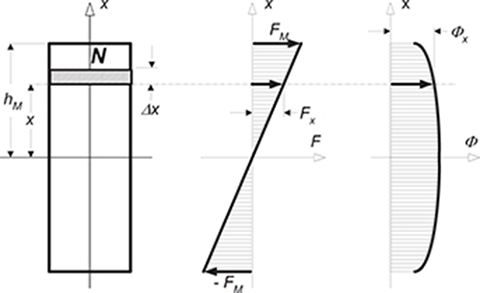
Fig. 2.10. Distribution of the MMF and magnetic flux along the height h_M of a rectangular PM.

H = 1 h M \int h M 0 H x d x = F M h M (2.12)

$H = \frac{1}{h_{M}} \int_{0}^{h_{M}} H_{x} d x = \frac{F_{M}}{h_{M}} (2.12)$

where H_x is the magnetic field intensity at a distance x from the neutral cross section, and F_M is the MMF of the PM per pole (MMF = 2F_M per pole pair).

The equivalent magnetic field intensity (2.12) allows the equivalent leakage flux of the PM to be found, i.e.,

Φ l M = Φ M - Φ g (2.13)

$Φ_{l M} = Φ_{M} - Φ_{g} (2.13)$

where Φ_M is the full equivalent flux of the PM, and Φ_g is the air gap magnetic flux. The coefficient of leakage flux of the PM,

σ l M = Φ M Φ g = 1 + Φ l M Φ g > 1 (2.14)

$σ_{l M} = \frac{Φ_{M}}{Φ_{g}} = 1 + \frac{Φ_{l M}}{Φ_{g}} > 1 (2.14)$

simply allows the air gap magnetic flux to be expressed as Φ_g = Φ_M/σ_lM.

The following leakage permeance expressed in the flux Φ-MMF coordinate system corresponds to the equivalent leakage flux of the PM:

G l M = Φ l M F M (2.15)

$G_{l M} = \frac{Φ_{l M}}{F_{M}} (2.15)$

An accurate estimation of the leakage permeance G_lM is the most difficult task in calculating magnetic circuits with PMs (Appendix A and Appendix B). This problem exists only in the circuital approach since using the field approach and, e.g., the finite element method (FEM), the leakage permeance can be found fairly accurately.

The average equivalent magnetic flux and equivalent MMF mean that the magnetic flux density and magnetic field intensity are assumed to be the same in the whole volume of a PM. The full energy produced by the magnet in the outer space is

W = B H 2 V M J (2.16)

$\begin{matrix} W = \frac{B H}{2} V_{M} & J \end{matrix} (2.16)$

where V_M is the volume of the PM or a system of PMs.

2.3.3 Magnetic Flux Density in the Air Gap

Let us consider a simple PM circuit with rectangular cross section consisting of a PM with height per pole h_M, width w_M, length l_M, two mild-steel yokes with average length 2l_Fe and an air gap of thickness g. From the Ampère’s circuital law,

2 H M h m = H g g + 2 H F e l F e = H g g (1 + 2 H F e l F e H g g) = H g k s a t

$2 H_{M} h_{m} = H_{g} g + 2 H_{F e} l_{F e} = H_{g} g (1 + \frac{2 H_{F e} l_{F e}}{H_{g} g}) = H_{g} k_{s a t}$

where H_g, H_Fe, and H_M are the magnetic field intensities in the air gap, mild steel yoke, and PM, respectively. The coefficient

k s a t = 1 + 2 H F e l F e H g g (2.17)

$k_{s a t} = 1 + \frac{2 H_{F e} l_{F e}}{H_{g} g} (2.17)$

takes into account the magnetic voltage drops in the mild steel and is called saturation factor of the magnetic circuit.

Since Φ_gσ_lM = Φ_M or B_gS_g = B_MS_M/σ_lM, where B_g is the air gap magnetic flux density, B_M is the PM magnetic flux density, S_g is the cross section area of the air gap, and S_M = w_Ml_M is the cross section area of the PM, the following equation can be written:

V M 2 h M 1 σ l M B M = μ 0 H g V g g

$\frac{V_{M}}{2 h_{M}} \frac{1}{σ_{l M}} B_{M} = μ_{0} H_{g} \frac{V_{g}}{g}$

where V_g = S_gg is the volume of the air gap, and V_M = 2h_MS_M is the volume of the PM. The fringing flux in the air gap has been neglected. Multiplying through the equation for magnetic voltage drops and for magnetic flux, the air gap magnetic flux intensity is found as

B g = μ 0 H g = μ 0 σ l M k - 1 s a t V M V g B M H M - - - - - - - - - - - - - - - - \sqrt (2.18)

$B_{g} = μ_{0} H_{g} = \sqrt{\frac{μ_{0}}{σ_{l M}} k_{s a t}^{- 1} \frac{V_{M}}{V_{g}} B_{M} H_{M}} (2.18)$

Assuming k_sat ≈ 1 and σ_lm ≈ 1,

B g \approx μ 0 V M V g B M H M - - - - - - - - - - - \sqrt (2.19)

$B_{g} \approx \sqrt{μ_{0} \frac{V_{M}}{V_{g}} B_{M} H_{M}} (2.19)$

For a PM circuit, the magnetic flux density B_g in a given air gap volume V_g is directly proportional to the square root of the energy product (B_MH_M) and the volume of magnet V_M = 2h_Mw_Ml_M.

Following the trend toward smaller packaging, smaller mass, and higher efficiency, the material research in the field of PMs has focused on finding materials with high values of the maximum energy product (BH)_max.

The air gap magnetic flux density B_g can be estimated analytically on the basis of the demagnetization curve, air gap, and leakage permeance lines and recoil lines (Appendix A). Approximately, for an LSM with armature ferromagnetic stack and surface configuration of PMs, it can be found on the basis of the balance of magnetic voltage drops that

B r μ 0 μ r r e c h M = B g μ 0 μ r r e c h M + B g μ 0 g

$\frac{B_{r}}{μ_{0} μ_{r r e c}} h_{M} = \frac{B_{g}}{μ_{0} μ_{r r e c}} h_{M} + \frac{B_{g}}{μ_{0}} g$

where μ_rrec is the relative permeability of the PM (relative recoil permeability). Hence,

B g = B r h M h M + μ r r e c g \approx B r 1 + μ r r e c g / h M (2.20)

$B_{g} = \frac{B_{r} h_{M}}{h_{M} + μ_{r r e c} g} \approx \frac{B_{r}}{1 + μ_{r r e c} g / h_{M}} (2.20)$

The air gap magnetic flux density is proportional to the remanent magnetic flux density B_r and decreases as the air gap g increases. Eqn (2.20) can only be used for preliminary calculations.

Demagnetization curves are sensitive to the temperature. Both B_r and H_c decrease as the magnet temperature increases, i.e.,

B r = B r 20 [1 + α B 100 (ϑ P M - 20)] (2.21)

$B_{r} = B_{r 20} [1 + \frac{α_{B}}{100} (ϑ_{P M} - 20)] (2.21)$

H c = H c 20 [1 + α H 100 (ϑ P M - 20)] (2.22)

$H_{c} = H_{c 20} [1 + \frac{α_{H}}{100} (ϑ_{P M} - 20)] (2.22)$

where ϑ_PM is the temperature of the PM, B_r20 and H_c20 are the remanent magnetic flux density and coercive force at 20°C, respectively, and α_B < 0 and α_H < 0 are temperature coefficients for B_r and H_c in %/⁰C, respectively.

2.3.4 Properties of Permanent Magnets

In electric motors technology, the following PM materials are used:

Alnico (Al, Ni, Co, Fe);
Ferrites (ceramics), e.g., barium ferrite BaO×6Fe₂ O₃ and strontium ferrite SrO×6Fe₂O₃;
Rare-earth materials, i.e., samarium—cobalt SmCo and neodymium— iron—boron NdFeB.

Images

Fig. 2.11. Demagnetization curves of different permanent magnet materials.

Demagnetization curves of these PM materials are given in Fig. 2.11.

The main advantages of Alnico are its high magnetic remanent flux density and low temperature coefficients. The temperature coefficient of B_r is −0.02%/^°C, and maximum service temperature is 520°C. These advantages allow a quite high air gap flux density and high operating temperatures. Unfortunately, coercive force is very low, and the demagnetization curve is extremely nonlinear. Therefore, it is very easy not only to magnetize but also to demagnetize Alnico. Sometimes, Alnico PMs are protected from the armature flux and, consequently, from demagnetization, using additional soft-iron pole shoes. Alnico magnets dominated the PM machines industry from the mid 1940s to about 1970 when ferrites became the most widely used materials [166].

Barium and strontium ferrites were invented in the 1950s. A ferrite has a higher coercive force than that of Alnico, but at the same time has a lower remanent magnetic flux density. Temperature coefficients are relatively high, i.e., the coefficient of B_r is −0.20%/^°C and the coefficient of H_c is −0.27%/^°C. The maximum service temperature is 400°C. The main advantages of ferrites are their low cost and very high electric resistance, which means no eddy-current losses in the PM volume. Barium ferrite PMs are commonly used in small d.c. commutator motors for automobiles (blowers, fans, windscreen wipers, pumps, etc.) and electric toys. Ferrites are produced by powder metallurgy. Their chemical formulation may be expressed as MO×6(Fe₂O₃), where M is Ba, Sr, or Pb. Strontium ferrite has a higher coercive force than barium ferrite. Lead ferrite has a production disadvantage from an environmental point of view. Ferrite magnets are available in isotropic and anisotropic grades.

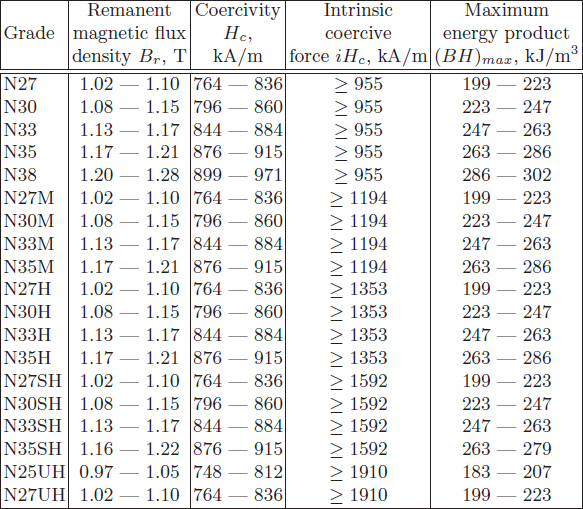
Table 2.9. Magnetic characteristics of sintered NdFeB PMs manufactured in China

Images

During the last three decades, great progress regarding available energy density (BH)_max has been achieved with the development of rare-earth PMs. The rare-earth elements are in general not rare at all, but their natural minerals are widely mixed compounds. To produce one particular rare-earth metal, several others, for which no commercial application exists, have to be refined. This limits the availability of these metals. The first generation of these new alloys were invented in the 1960s and based on the composition SmCo₅, which has been commercially produced since the early 1970s. Today it is a well established hard magnetic material. SmCo₅ has the advantage of high remanent flux density, high coercive force, high energy product, linear demagnetization curve, and low temperature coefficient. The temperature coefficient of B_r is −0.03%/°C to −0.045%/°C, and the temperature coefficient of H_c is −0.14%/°C to −0.40%/°C. Maximum service temperature is 250° to 300°C. It is well suited to build motors with low volume and, consequently, high specific power and low moment of inertia. The cost is the only drawback. Both Sm and Co are relatively expensive due to their supply restrictions.

With the discovery of a second generation of rare-earth magnets on the basis of cost-effective neodymium (Nd) and iron (Fe), a remarkable progress with regard to lowering raw material costs has been achieved. This new generation of rare-earth PMs was announced by Sumitomo Special Metals, Japan, in 1983 at the 29th Annual Conference of Magnetism and Magnetic Materials held in Pittsburg. The Nd is a much more abundant rare-earth element than Sm. NdFeB magnets, which are now produced in increasing quantities, have better magnetic properties than those of SmCo, but unfortunately only at room temperature. The demagnetization curves, especially the coercive force, are strongly temperature dependent. The temperature coefficient of B_r is −0.095%/°C to −0.15%/°C and the temperature coefficient of H_c is −0.40%/°C to −0.70%/°C. The maximum service temperature is 170⁰C, and Curie temperature is 300 to 360°C. The NdFeB is also susceptible to corrosion. NdFeB magnets have great potential for considerably improving the performance–to–cost ratio for many applications. For this reason they have a major impact on the development and application of PM apparatus.

Table 2.10. Physical properties of sintered NdFeB PMs manufactured in China

Images

Table 2.11. Magnetic characteristics of bonded NdFeB PMs manufactured in China

Images

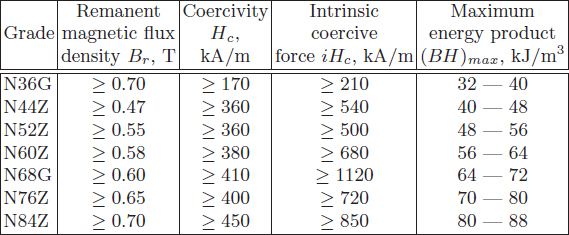
Table 2.12. Physical properties of bonded NdFeB PMs manufactured in China

Images

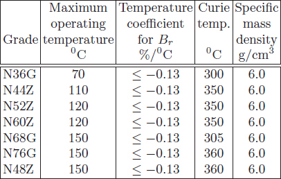
According to the manufacturing processes, rare earth NdFeB PMs are clasified into sintered PMs (Tables 2.9 and 2.10) and bonded PMs (Table 2.11 and 2.12).

2.4 Conductors

Armature windings of electric motors are made of solid copper conductor wires with round or rectangular cross sections. When the cost or mass of the motor are paramount, e.g., long armature LSMs for transportation systems, magnetically levitated vehicles, hand tools, etc., aluminum conductor wires can be more suitable.

2.4.1 Magnet Wire

The magnet wire or winding wire is an insulated copper or aluminum conductor typically used to wind electromagnetic devices such as machines and transformers. American Wire Gauge is the standard used to represent successive diameters of wire. The system is based on the establishment of two arbitrary sizes: 4/0 defined exactly as 0.4600 inch diameter, and 36, defined as exactly 0.0050 inch diameter. The ratio of these two sizes is 92, and the sizes, between the two are based on the 39th root of 92, or approximately 1.123, so the nominal diameter of each gauge size increases approximately by this factor between AWG 36 and AWG 4/0, and decreases by this factor between AWG 36 and AWG 56, which is the smallest practical diameter for commercial magnet wire. Nominal wire diameters to AWG 44 are rounded to the fourth decimal place and are not necessarily rounded to the nearest digit.

There are a number of film insulation types ranging from temperature Class 105°C to Class 240°C. Each film type has its own unique set of characteristics to suit specific needs of the user. A very common wire used in many applications is single build polyurethane Class 155°C with a nylon topcoat. It is stocked in most sizes and is a good general-purpose insulation for undecided customers. Armored polyester insulation is another option when a higher temperature class is desired.

Bondable wire has a thermoplastic adhesive film superimposed over standard film insulation. When activated by heat or solvent, the bond coating cements the winding turn-to-turn to create a self-supporting coil. The use of bondable wire can eliminate the need for bobbins, tape, or varnishes.

2.4.2 Resistivity and Conductivity

Electric conductivity σ of materials used for windings of electrical machines is given in Table 2.13. The electric conductivity is temperature dependent.

The variation of resistance R, electric resistivity ρ and electric conductivity σ with temperature in temperature range from 0°C to 150°C is expressed by the following equations:

R (ϑ) = R 20 [1 + α 20 (ϑ - 20)] (2.23)

$R (ϑ) = R_{20} [1 + α_{20} (ϑ - 20)] (2.23)$

ρ (ϑ) = ρ 20 [1 + α 20 (ϑ - 20)] (2.24)

$ρ (ϑ) = ρ_{20} [1 + α_{20} (ϑ - 20)] (2.24)$

σ (ϑ) = σ 20 1 + α 20 ( ϑ - 20 ) (2.25)

$σ (ϑ) = \frac{σ_{20}}{1 + α_{20} (ϑ - 20)} (2.25)$

where R₂₀, ρ₂₀, σ₂₀, α₂₀ are the resistance, resistivity, conductivity, and temperature coefficient at 20°C, respectively, and ϑ is the given temperature. For copper wires, α = 0.00393 1/⁰C, and for aluminum wires α = 0.00403 1/⁰C. For ϑ > 150°C, additional electric temperature coefficient β₂₀ must be introduced, e.g., for resistance

R ϑ = R 20 [1 + α 20 (ϑ - 20) + β 20 (ϑ - 20) 2] (2.26)

$R_{ϑ} = R_{20} [1 + α_{20} (ϑ - 20) + β_{20} {(ϑ - 20)}^{2}] (2.26)$

At temperatures higher than room temperature (up to 1000°C), the resistivity of copper, aluminum, and brass changes more or less linearly with temperature, while the resistivity of steels abruptly increases (Fig. 2.12).

Images

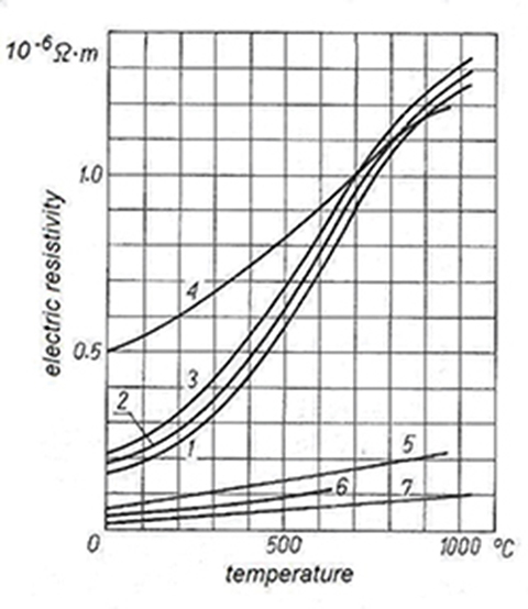
Fig. 2.12. Variation of resistivity ρ of metals with temperature: 1 — mild steel 0.11%C, 2 — mild steel 0.5%C, 3 — mild steel 1% C, 4 — stainless and acid resistant steels, 5 — brass 60%Cu, 6 — aluminum, 7 — copper [126].

Table 2.13. Electric resistivity, conductivity, and temperature coefficient at 20°C

Images

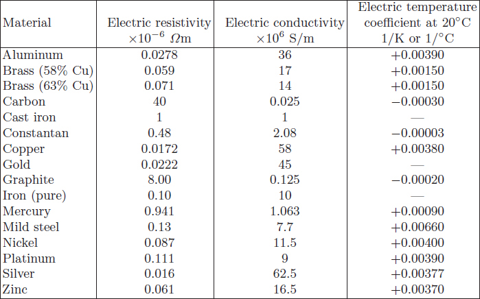
Normally, the resistivity of copper used for electric conductors is ρ = 0.017241 × 10⁻⁶ Ωm at 20°C, conductivity σ = 58 × 10⁶ S/m, the specific mass density 8900 kg/m³, coefficient of linear expansion 1.68 × 10⁻⁵ 1/K, specific heat to 390 Ws/K, and unit heat conductivity 3.75 × 10² W/(K m). Various impurities degrade the electrical conductivity of copper.

The resitivity of aluminum, in normally refined form, is ρ = 0.0282 × 10⁻⁶ Ωm at 20°C, conductivity σ = 35.5 × 10⁶ S/m, specific mass density 2640 kg/m³ for cast aluminum, 2700 kg/m³ for drawn aluminum, coefficient of linear expansion 2.22 × 10⁻⁵ 1/K, specific heat 810 Ws/K, and unit heat conductivity 2.0 × 10² W/(K m).

Table 2.14. Maximum temperature rise Δϑ for armature windings of electrical machines according to IEC and NEMA (based on 40^o ambient temperature)

Images

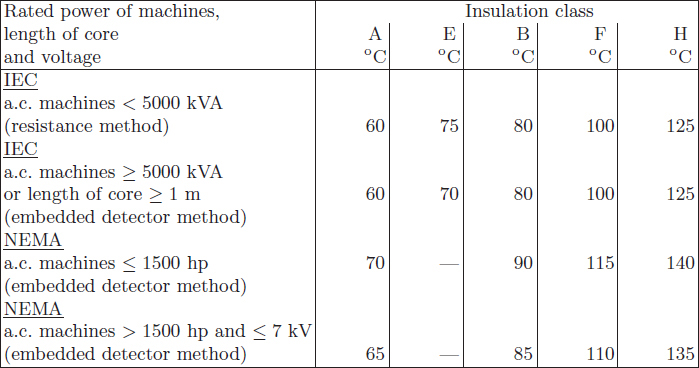
Table 2.15. Magnet wire insulation summary

Images

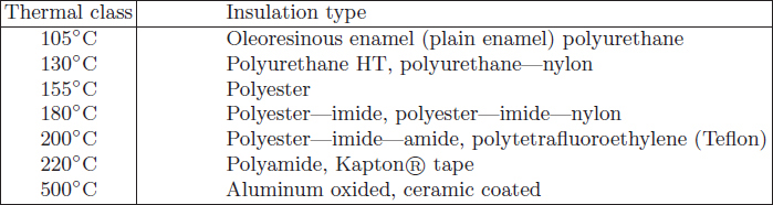
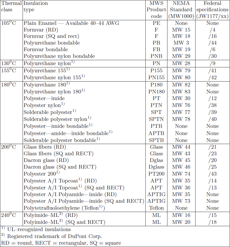
Table 2.16. Insulation specifications according to MWS Wire Industries, www.mwswire.com

Images

2.5 Insulation Materials

2.5.1 Classes of Insulation

The maximum temperature rise for the windings of electrical machines is determined by the temperature limits of insulating materials. The maximum temperature rise in Table 2.14 assumes that the temperature of the cooling medium ϑ_c ≤ 40⁰C. The winding can reach the maximum temperature of

ϑ max = ϑ c + Δ ϑ (2.27)

$ϑ_{max} = ϑ_{c} + Δ ϑ (2.27)$

where Δϑ is the maximum allowable temperature rise according to Table 2.14. Polyester–imide and polyamide–imide coat can provide operating temperature of 200⁰C.

2.5.2 Commonly Used Insulating Materials

Magnet wire insulation summary is given in Table 2.15. Insulation specifications according to MWS Wire Industries, Westlake Village, CA are listed in Table 2.16.

Heat-sealable Kapton® polyimide films are used as primary insulation on magnet wire at temperatures 220°C to 240°C [154]. These films are coated with or laminated to Teflon® fluorinated ethylene propylene (FEP) fluo-ropolymer, which acts as a high-temperature adhesive. The film is applied in tape form by helically wrapping it over and heat-sealing it to the conductor and to itself.

The highest operating temperatures (over 600⁰C) can be achieved using nickel clad copper or palladium–silver conductor wires and ceramic insulation [34].

2.5.3 Impregnation

After coils are wound, they must be somehow secured in place so as to avoid conductor movement. Two standard methods are used to secure the conductors of electrical machines in place:

Dipping the whole component into a varnish-like material, and then baking off its solvent
Trickle impregnation method, which uses heat to cure a catalyzed resin that is dripped onto the component

Polyester, epoxy, or silicon resins are most often used as impregnating materials for treatment of stator or rotor windings. Silicon resins of high thermal endurance are able to withstand ?_max > 225°C.

Recently, a new method of conductor securing that does not require any additional material and uses very low energy input has emerged [132]. The solid conductor wire (usually copper) is coated with a heat- and/or solvent-activated adhesive. The adhesive, which is usually a polyvinyl butyral, utilizes a low-temperature thermoplastic resin [132]. This means that the bonded adhesive can come apart after a certain minimum temperature is reached, or it again comes in contact with the solvent. Normally, this temperature is much lower than the thermal rating of the base insulation layer. The adhesive is activated by either passing the wire through a solvent while winding or heating the finished coil as a result of passing electric current through it.

The conductor wire with a heat-activated adhesive overcoat costs more than the same class of nonbondable conductor. However, a less than two second current pulse is required to bond the heat-activated adhesive layer, and bonding machinery costs about half as much as trickle impregnation machinery [132].

Polyester, epoxy, or silicon resins are used most often as impregnating materials for the treatment of stator windings. Silicon resins of high thermal endurance are able to withstand ?_max > 225°C.

2.6 Principles of Superconductivity

Superconductivity (SC) is a phenomenon occurring in certain materials at low temperatures, characterized by the complete absence of electrical resistance and the damping of the interior magnetic field (Meissner effect). The critical temperature for SCs is the temperature at which the electrical resistivity of an SC drops to zero. Some critical temperatures of metals are aluminum (Al) T_c = 1.2 K, tin (Sn) T_c = 3.7 K, mercury (Hg) T_c = 4.2 K, vanadium (V) T_c = 5.3 K, lead (Pb) T_c = 7.2 K, niobium (Nb) T_c = 9.2 K. Compounds can have higher critical temperatures, e.g., T_c = 92 K for YBa₂Cu₃O₇, and T_c = 133 K for HgBa₂Ca₂Cu₃O₈. Superconductivity was discovered by the Dutch scientist H. Kamerlingh Onnes in 1911 (Nobel Prize in 1913). Onnes was the first person to liquefy helium (4.2 K) in 1908.

The superconducting state is defined by three factors (Fig. 2.13):

Critical temperature T_c;
Critical magnetic field H_c;
Critical current density J_c.

Maintaining the superconducting state requires that both the magnetic field and the current density, as well as the temperature, remain below the critical values, all of which depend on the material.

The phase diagram T_cH_cJ_c shown in Fig. 2.13 demonstrates the relationship between T_c, H_c, and J_c. When considering all three parameters, the plot represents a critical surface. For most practical applications, SCs must be able to carry high currents and withstand high magnetic field without reverting to their normal state.

Images

Fig. 2.13. Phase diagram T_cH_cJ_c.

Meissner effect (sometimes called the Meissner—Ochsenfeld effect) is the expulsion of a magnetic field from an SC.

When a thin layer of insulator is sandwiched between two SCs, until the current becomes critical, electrons pass through the insulator as if it does not exist. This effect is called Josephson effect. This phenomenon can be applied to the switching devices that conduct on—off operation at high speed.

In type I superconductors, the superconductivity is “quenched” when the material is exposed to a sufficiently high magnetic field. This magnetic field, H_c, is called the critical field. In contrast, type II superconductors have two critical fields. The first is a low-intensity field H_c1, which partially suppresses the superconductivity. The second is a much higher critical field, H_c2, which totally quenches² the superconductivity. The upper critical field of type II superconductors tends to be two orders of magnitude or more above the critical fields of a type I superconductor.

Some consequences of zero resistance are as follows:

When a current is induced in a ring-shaped SC, the current will continue to circulate in the ring until an external influence causes it to stop. In the 1950s, “persistent currents” in SC rings immersed in liquid helium were maintained for more than 5 years without the addition of any further electrical input.
An SC cannot be shorted out. If the effects of moving a conductor through a magnetic field are ignored, then connecting another conductor in parallel, e.g., a copper plate across an SC, will have no effect at all. In fact, by comparison to the SC, copper is a perfect insulator.
The diamagnetic effect that causes a magnet to levitate above an SC is a complex effect. Part of it is a consequence of zero resistance and of the fact that an SC cannot be shorted out. The act of moving a magnet toward an SC induces circulating persistent currents in domains in the material. These circulating currents cannot be sustained in a material of finite electrical resistance. For this reason, the levitating magnet test is one of the most accurate methods of confirming superconductivity.
Circulating persistent currents form an array of electromagnets that are always aligned in such as way as to oppose the external magnetic field. In effect, a mirror image of the magnet is formed in the SC with a North pole below a North pole and a South pole below a South pole.

The main factor limiting the field strength of the conventional (Cu or Al wire) electromagnet is the I²R power losses in the winding when sufficiently high current is applied. In an SC, in which R ≈ 0, the I²R power losses practically do not exist.

Lattice (from the mathematics point of view) is a partially ordered set in which every pair of elements has a unique supremum (least upper bound of elements, called their join) and an infimum (greatest lower bound, called their meet). Lattice is an infinite array of points in space, in which each point has surroundings identical to all others. Crystal structure is the periodic arrangement of atoms in the crystal.

The only way to describe SCs is to use quantum mechanics. The model used is the BSC theory (named after Bardeen, Cooper, and Schrieffer) was first suggested in 1957 (Nobel Prize in 1973) [20]. It states that

lattice vibrations play an important role in superconductivity;
electron—phonon interactions are responsible.

Photons are the quanta of electromagnetic radiation. Phonons are the quanta of acoustic radiation. They are emitted and absorbed by the vibrating atoms at the lattice points in the solid. Phonons possess discrete energy E = hv, where h = 6.626 068 96(33) × 10⁻³⁴ Js is Planck constant. Phonons propagate through a crystal lattice.

Low temperatures minimize the vibrational energy of individual atoms in the crystal lattice. An electron moving through the material at low temperature encounters less of the impedance due to vibrational distortions of the lattice. The Coulomb attraction between the passing electron and the positive ion distorts the crystal structure. The region of increased positive charge density propagates through the crystal as a quantized sound wave called a phonon. The phonon exchange neutralizes the strong electric repulsion between the two electrons due to Coulomb forces. Because the energy of the paired electrons is lower than that of unpaired electrons, they bind together. This is called Cooper pairing. Cooper pairs carry the supercurrent relatively unresisted by the thermal vibration of the lattice. Below T_c, pairing energy is sufficiently strong (Cooper pair is more resistant to vibrations), the electrons retain their paired motion and, upon encountering a lattice atom, do not scatter. Thus, the electric resistivity of the solid is zero. As the temperature rises, the binding energy is reduced and goes to zero when T = T_c. Above T_c, a Cooper pair is not bound. An electron alone scatters (collision interactions), which leads to ordinary resistivity. Conventional conduction is resisted by thermal vibration within the lattice.

Images

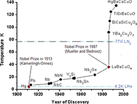
Fig. 2.14. Discovery of materials with successively higher critical temperatures over the last century.

In 1986, J. Georg Bednorz and K. Alex Mueller of IBM Ruschlikon, Switzerland, published results of research [23] showing indications of superconductivity at about 30 K (Nobel Prize in 1987). In 1987 researchers at the University of Alabama at Huntsville (M. K. Wu) and at the University of Houston (C. W. Chu) produced ceramic SCs with a critical temperature (T_c = 52.5 K) above the temperature of liquid nitrogen. Discoveries of materials with successively higher critical temperatures over the last century are presented in Fig. ??.

There is no widely accepted temperature that separates high-temperature superconductors (HTS) from low-temperature superconductors (LTS). Most LTS superconduct at the boiling point of liquid helium (4.2 K = −269⁰C at 1 atm). However, all the SCs known before the 1986 discovery of the supercon-ducting oxocuprates would be classified LTS. The barium-lanthanum-cuprate BaLaCuO fabricated by Mueller and Bednorz, with a T_c = 30 K = −243⁰C, is generally considered to be the first HTS material. Any compound that will su-perconduct at and above this temperature is called HTS. Most modern HTS superconduct at the boiling point of liquid nitrogen (77 K = −196⁰C at 1 atm).

The most important market for LTS electromagnets are currently magnetic resonance imaging (MRI) devices, which enable physicians to obtain detailed images of the interior of the human body without surgery or exposure to ionizing radiation.

All HTS are cuprates (copper oxides). Their structure relates to the perovskite structure (calcium titanium oxide CaTiO₃) with the general formula ABX₃. Perovskite CaTiO₃ is a relatively rare mineral occurring in orthorhombic (pseudocubic) crystals³.

With the discovery of HTS in 1986, the US almost immediately resurrected interest in superconducting applications. The US Department of Energy (DoE) and Defense Advanced Research Projects Agency (DARPA) have taken the lead in the research and development of electric power applications. At 60 to 77 K (liquid nitrogen), thermal properties become more friendly, and cryogenics can be 40 times more efficient than at 4.2 K (liquid helium).

In power engineering, superconductivity can be practically applied to synchronous machines, homopolar machines, transformers, energy storages, transmission cables, fault-current limiters, LSMs, and magnetic levitation vehicles. The use of superconductivity in electrical machines reduces the excitation losses, increases the magnetic flux density, eliminates ferromagnetic cores, and reduces synchronous reactance (in synchronous machines).

The apparent electromagnetic power is proportional to electromagnetic loadings, i.e., the stator line current density and the air gap magnetic flux density. High magnetic flux density increases the output power or reduces the size of the machine. Using SCs for field excitation winding, the magnetic flux density can exceed the saturation magnetic flux of the best ferromagnetic materials. Thus, ferromagnetic cores can be removed.

2.7 Superconducting Wires

The first commercial low LTS wire was developed at Westinghouse in 1962. Typical LTS wires are magnesium diboride MgB₂ tapes, NbTi Standard, and Nb₃Sn Standard. LTS wires are still preferred in high field magnets for nuclear magnetic resonance (NMR), magnetic resonance imaging (MRI), magnets for accelerators, and fusion magnets. Input cooling power as a function of required temperature is shown in Fig. 2.15.

Images

Fig. 2.15. Input cooling power in percent of requirements at 4.2K versus temperature.

Manufacturers of electrical machines need low-cost HTS tapes that can operate at temperatures approaching 77 K for economical generators, motors, and other power devices. The minimum length of a single piece acceptable by the electrical engineering industry is at least 100 m.

2.7.1 Classification of HTS Wires

HTSwires are divided into two categories:

First generation (1G) superconductors, i.e., multifilamentary tape conductors BiSrCaCuO (BSCCO) developed up to industrial state. Their properties are reasonable for different use, but prices are still high.
Second generation (2G) superconductors, i.e., coated tape conductors: YBaCuO (YBCO) which offer superior properties.

Fig. 2.16 shows basic 1G and 2G HTS wire tape architecture according to American Superconductors [10]. Each type of advanced wire achieves high power density with minimal electrical resistance, but differs in the SC materials manufacturing technology, and, in some instances, its end-use applications.

Parameters characterizing superconductors are

critical current I_c × (wire length), Am (200, 580 Am in 2008) [196];
critical current I_c/(wire width), A/cm–width (700 A/cm–width in 2009) [10];
engineering critical current density J_e, A/cm²;
critical current density J_c, A/cm².

The engineering critical current density J_e is the critical current of the wire divided by the cross sectional area of the entire wire, including both superconductor and other metal materials.

Images

Fig. 2.16. HTS wires: (a) 1st generation (1G); (b) 2nd generation (2G). 1 — silver alloy matrix, 2 — SC filaments, 3 — SC coating, 4 — buffer layer, 5 — noble metal layer, 5 — alloy substrate.

BSCCO 2223 is a commonly used name to represent the HTS material Bi_(2−x)Pb_xSr₂Ca₂Cu₃O₁₀. This material is used in multifilamentary composite HTS wire and has a typical superconducting transition temperature around 110 K. BSCCO-2223 is proving successful presently but will not meet all industrial requirements in the nearest future. According to SuperPower [196], there are clear advantages to switch from 1G to 2G,

better in-field performance;
better mechanical properties (higher critical tensile stress, higher bend strain, higher tensile strain);
better uniformity, consistency, and material homogeneity;
higher engineering current density;
lower a.c. losses.

There are key areas where 2G needs to be competitive with 1G in order to be used in the next round of various device prototype projects. Key benchmarks to be addressed are

long piece lengths;
critical current over long lengths;
availability (high throughput, i.e., production volume per year, large deliveries from pilot-scale production);
comparable cost with 1G.

Commercial quantities of HTS wire based on BSCCO are now available at around five times the price of the equivalent copper conductor. Manufacturers are claiming the potential to reduce the price of YBCO to 50% or even 20% of BSCCO. If the latter occurs, HTS wire will be competitive with copper in many large industrial applications.

Magnesium diboride, MgB₂, is a much cheaper SC than BSCCO and YBCO in terms of dollars per current-carrying capacity × length ($/kA-m). However, this material must be operated at temperatures below 39K, so the cost of cryogenic equipment is very significant. This can be half the capital cost of the electric machine when cost-effective SC is used. Magnesium di-boride, SC MgB₂, might gain niche applications if further developments will be successful.

As of March 2007, the current world record of superconductivity is held by a ceramic SC consisting of thallium, mercury, copper, barium, calcium, strontium, and oxygen with T_c = 138 K.

2.7.2 HTS Wires Manufactured by American Superconductors

American Superconductors (AMSC) [10] is the world’s leading developer and manufacturer of HTS wires. Two types of HTS wires branded as 344 and 348 have been commercially available since 2005. AMSC HTS wire specifications are given in Table 2.17.

Table 2.17. Specifications of HTS wires manufactured by American Superconductors, Westborough, MA, USA [10]

Images

Today, AMSC 2G HTS wire manufacturing technology is based on 100-m long, 4-cm wide strips of SC material that are produced in a high-speed, continuous reel–to–reel deposition⁴ process, the so-called rolling assisted bi-axially textured substrates (RABITS). RABITS is a method for creating textured⁵ metal substrate for 2G wires by adding a buffer layer between the nickel substrate and YBCO. This is done to prevent the texture of the YBCO from being destroyed during processing under oxidizing atmospheres. This process is similar to the low-cost production of motion picture film in which celluloid strips are coated with a liquid emulsion and subsequently slit and laminated into eight, industry-standard 4.4-mm wide tape-shaped wires (344 SCs). The wires are laminated on both sides with copper or stainless-steel metals to provide strength, durability, and certain electrical characteristics needed in applications. AMSC expects to scale up the 4 cm technology to 1000-m lengths. The company then plans to migrate to 10 cm technology to further reduce manufacturing costs.

Sumitomo Electric Industries, Japan, uses the holmium (Ho) rare element instead of yttrium (Y). According to Sumitomo, the HoBCO SC layer allows for higher rate of deposition, high critical current density J_c, and better flexibility of tape than the YBCO SC layer.

2.7.3 HTS Wires Manufactured by SuperPower

SuperPower [196] uses ion beam assisted deposition (IBAD), a technique for depositing thin SC films. IBAD combines ion implantation with simultaneous sputtering or another physical vapor deposition (PVD) technique. An ion beam is directed at an angle toward the substrate to grow textured buffer layers. According to SuperPower, virtually, any substrate could be used, i.e., high-strength substrates, nonmagnetic substrates, low-cost, off–the–shelf substrates (Inconel, Hastelloy, stainless steel), very thin substrates, resistive substrates (for low a.c. losses), etc. There are no issues with percolation (trickling or filtering through a permeable substance). IBAD can pattern the conductor to very narrow filaments for a low a.c. loss conductor. An important advantage is small grain size in the submicron range.

IBAD MgO—based coated conductor has five thin oxide buffer layers with different functions, such as

alumina barrier layer to prevent diffusion of metal element into SC;
yttria seed layer to provide good nucleation surface for IBAD MgO;
IBAD MgO template layer to introduce biaxial texture;
homoepitaxial MgO buffer layer to improve biaxial texture;
SrTiO₃ (STO) cap layer to provide lattice match between MgO and YBCO and good chemical compatibility.

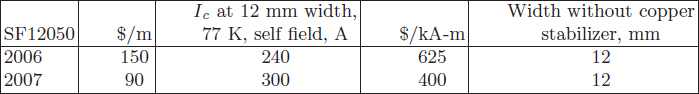
Tables 2.18 and 2.19 show the cost and selected specifications of HTS 2G tapes manufactured by SuperPower [196].

Table 2.18. Cost per meter and parameters of SCS4050 4 mm HTS tape [196].

Images

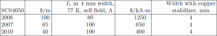
Table 2.19. Cost per meter and parameters of SF12050 12 mm HTS tape [196].

Images

2.8 Laminated Stacks

Most LSMs use laminated armature stacks with rectangular semiopen or open slots. In low-speed industrial applications, the frequency of the armature current is well below the power frequency 50 or 60 Hz so that, from the electromagnetic point of view, laminations can be thicker than 0.5 or 0.6 mm (typical thickness for 50 or 60 Hz, respectively). The laminations are cut to dimensions using stamping presses in mass production or laser cutting machines when making prototypes of LSMs. If the stack is thicker than 50 mm, it is recommended that laminations be grouped into 20 to 40-mm thick packets separated by 4 to 8-mm wide longitudinal cooling ducts. Each of the two external laminations should be thicker than internal laminations to prevent the expansion (swelling) of the stack at toothed edges. The slot pitch of a flat armature core is

t 1 = b 11 + c t = 2 p τ / s 1 (2.28)

$t_{1} = b_{11} + c_{t} = 2 p τ / s_{1} (2.28)$

where b₁₁ is the width of the rectangular slot, c_t is the width of tooth, 2p is the number of poles, τ is the pole pitch, and s₁ is the number of slots totally filled with conductors. The shapes of armature slots of flat LSMs are shown in Fig. 2.17.

The laminations are kept together with the aid of seam welds (Fig. 2.18), spot welds, or using bolts and bars pressing the stack (Fig. 2.19).

Stamping and stacking can be simplified by using rectangular laminations, as in Fig. 2.20 [227]. When making a prototype, the laminated stack of a polyphase LSM can also be assembled of E-shaped laminations, the same as those used in manufacturing small single-phase transformers.

Images

Fig. 2.17. Armature slots of flat LSMs: (a) semiopen, (b) open.

For slotless windings, armature stacks are simply made of rectangular strips of electrotechnical steel.

LSMs for heavy-duty applications are sometimes furnished with finned heat exchangers or water-cooled cold plates that are attached to the yoke of the armature stack.

Armature stacks of tubular motors can be assembled in the following three ways by using

star ray arranged long flat slotted stacks of the same dimensions that embrace the excitation system;
modules of ring laminations with inner different diameters for teeth and for slots;
sintered powders.

The last method seems to be the best from the point of view of performance of the magnetic circuit.

Images

Fig. 2.18. Laminated stack assembled with the aid of seam welds.

Images

Fig. 2.19. Laminated stack assembled by using: 1 — bolts, and 2 — pressing angle bars.

Images

Fig. 2.20. Slotted armature stack of an a.c. linear motor assembled of rectangular laminations.

2.9 Armature Windings of Slotted Cores

Armature windings are usually made of insulated copper conductors. The cross section of conductors can be circular or rectangular. Sometimes, to obtain a high power density, a direct water-cooling system has to be used, and consequently, hollow conductors.

It is difficult to make and shape armature coil if the round conductor is thicker that 1.5 mm. If the current density is too high, parallel conductor wires of smaller diameter are recommended rather than one thicker wire. Armature windings can also have parallel current paths.

Armature windings can be either single layer or double layer. Fig. 2.21 shows a three-phase, four-pole winding configured both as double-layer and single-layer windings. In Fig. 2.21a, the number of slots s₁ = 24 assumed for calculations is equal to the number of slots totally filled with conductors, i.e. 19 plus 50% of half filled slots, which is 19 + 0.5 × 10 = 24. The total number of slots is [63]

s' 1 = 1 2 p (2 p + w c τ) s 1 = 1 4 (4 + 5 6) 24 = 29

${s^{'}}_{1} = \frac{1}{2 p} (2 p + \frac{w_{c}}{τ}) s_{1} = \frac{1}{4} (4 + \frac{5}{6}) 24 = 29$

where w_c ≤ τ is the coil pitch.

Double-layer armature winding wound with rectangular cross section of conductors of a large-power flat LSM is shown in Fig. 2.22. The coil pitch is equal to three slots, three end slots are half filled, and the end turns are diamond-shaped.

Armature windings of long-core, large-power LSMs can be made of cable. For example, the German Transrapid maglev system uses a multistrand, very soft aluminum conductor of 300 mm² cross section. The insulation consists of a synthetic elastometer with small dielectric losses. Inner and outer conductive films limit the electric field to the space of the insulation. The cable has a conductive sheath, also consisting of an elastometer mixture, for external protection and electric shielding.

The resistance of a flat armature winding as a function of the winding parameters, dimensions, and electric conductivity is expressed as

R 1 = 2 ( L ' i k 1 R + l 1 e ) N 1 σ s w 1 a w a p (2.29)

$R_{1} = \frac{2 ({L^{'}}_{i} k_{1 R} + l_{1 e}) N_{1}}{σ s_{w 1} a_{w} a_{p}} (2.29)$

where N₁ is the number of series turns per phase, L'_i is the length of the laminated stack including cooling ducts, l_1e is the average length of a single end connection, k_1R is the skin effect coefficient (k_1R ≈ 1 for round conductors with diameter less than 1 mm and frequency 50 to 60 Hz), σ is the electric conductivity of the conductor at the operating temperature — eqn (2.25), s_w1 is the cross section of the armature conductor wire, a_w is the number of parallel conductors, and a_p is the number of parallel current paths. For tubular LSMs, l_1e = 0 and 2L'_i in the numerator should be replaced by an average length of turn l_1av = π(D_1in + h₁) or l_1av = π(D_1out − h₁), where h₁ is the height of the concentrated primary coil, D_1in is the inner diameter of the armature stack, and D_1out is the outer diameter of the armature stack.

Images

Fig. 2.21. Three-phase, four-pole (2p = 4) full pitch windings of an LSM distributed in 24 slots: (a) double-layer winding; (b) single-layer winding.

Images

Fig. 2.22. Double-layer winding wound with rectangular cross section wires of a large PM LSM. Photo courtesy of Dr. S. Kuznetsov, Power Superconductor Applications Corp., Pittsburgh, PA, USA.

A more accurate method of calculating the armature resistance of a tubular a.c. linear motor is given below. For a ring-shaped coil consisting of n layers of rectangular conductor with its height h_wir = h₁/n, the length of the conductor per coil is expressed by the following arithmetic series:

2 π (r + h w i r) + 2 π (r + 2 h w i r) + 2 π (r + 3 h w i r) + \dots + 2 π (r + n h w i r) = 2 π r n + 2 π (h w i r + 2 h w i r + 3 h w i r + \dots + n h w i r) = 2 π n (r + h w i r 1 + n 2)

$\begin{matrix} 2 π (r + h_{w i r}) + 2 π (r + 2 h_{w i r}) + 2 π (r + 3 h_{w i r}) + \dots + 2 π (r + n h_{w i r}) \\ = 2 π r n + 2 π (h_{w i r} + 2 h_{w i r} + 3 h_{w i r} + \dots + n h_{w i r}) = 2 π n (r + h_{w i r} \frac{1 + n}{2}) \end{matrix}$

where the sum of the arithmetic series is S_n = n(a₁ + a_n)/2, the first term a₁ = h_wir, the last term a_n = nh_wir, and the inner radius of the coil is

r = D 1 i n + 2 ( h 14 + h 13 + h 12 ) 2 (2.30)

$r = \frac{D_{1 i n} + 2 (h_{14} + h_{13} + h_{12})}{2} (2.30)$

where h₁₄ is the slot opening, and h₁₃ and h₁₂ are dimensions according to Fig. 2.17. For the whole phase winding the length of the conductor per phase is

s 1 m 1 2 π n (r + h w i r 1 + n 2)

$\frac{s_{1}}{m_{1}} 2 π n (r + h_{w i r} \frac{1 + n}{2})$

where s₁ is the number of the armature slots, and s₁/m₁ is the number of cylindrical coils per phase in the case of an m₁ phase winding. The resistance of the armature winding per phase is

R 1 = s 1 m 1 π N s l a w \times [D 1 i n + 2 (h 14 + h 13 + h 12) + h w i r (1 + N s l a w)] k 1 R σ h w i r b w i r a w a p (2.31)

$R_{1} = \frac{s_{1}}{m_{1}} π \frac{N_{s l}}{a_{w}} \times [D_{1 i n} + 2 (h_{14} + h_{13} + h_{12}) + h_{w i r} (1 + \frac{N_{s l}}{a_{w}})] \frac{k_{1 R}}{σ h_{w i r} b_{w i r} a_{w} a_{p}} (2.31)$

where h_wir is the height of the rectangular conductor, b_wir is the width of the conductor, σ is the electric conductivity of the conductor, N_sl is the number of conductors per slot, a_w is the number of parallel wires, n = N_sl/a_w provided that parallel wires are located beside each other, and a_p is the number of parallel current paths. It is recommended that the cross section area of the conductor in the denominator be multiplied by a factor 0.92 to 0.99 to take into account the round corners of rectangular conductors. The bigger the cross section of the conductor, the bigger the factor including round corners. Eqn (2.31) should always be adjusted for the arrangement of conductor wires in slots.

The armature leakage reactance is the sum of the slot leakage reactance X_1s, the end connection leakage reactance X_1e, and the differential leakage reactance X_1d (for higher space harmonics), i.e.,

X 1 = X 1 s + X 1 e + X 1 d = 4 π f μ 0 L i N 2 1 p q 1 (λ 1 s k 1 X + l 1 e L i λ 1 e + λ 1 d + λ 1 t) (2.32)

$X_{1} = X_{1 s} + X_{1 e} + X_{1 d} = 4 π f μ_{0} \frac{L_{i} N_{1}^{2}}{p q_{1}} (λ_{1 s} k_{1 X} + \frac{l_{1 e}}{L_{i}} λ_{1 e} + λ_{1 d} + λ_{1 t}) (2.32)$

where N₁ is the number of turns per phase, k_1X is the skin-effect coefficient for leakage reactance, p is the number of pole pairs, q₁ = s₁/(2pm₁) is the number of primary slots s₁ per pole per phase, l_1e is the length of the primary winding end connection, λ_1s is the coefficient of the slot leakage permeance (slot-specific permeance), λ_1e is the coefficient of the end turn leakage permeance, and λ_1d is the coefficient of the differential leakage. For a tubular LSM, λ_1e = 0, and L_i should be replaced by L_i = π(D_1in + h₁) or L_i = π(D_1out − h₁). There is no leakage flux about the end connections as they do not exist in tubular LIMs.

The coefficients of leakage permeances of the slots shown in Fig. 2.17 are:

for a semiopen slot (Fig. 2.17a)

$λ 1 s = h 11 3 b 11 + h 12 b 11 + 2 h 13 b 11 + b 14 + h 14 b 14 (2.33)$ $λ_{1 s} = \frac{h_{11}}{3 b_{11}} + \frac{h_{12}}{b_{11}} + \frac{2 h_{13}}{b_{11} + b_{14}} + \frac{h_{14}}{b_{14}} (2.33)$
for an open slot (Fig. 2.17b)

$λ 1 s \approx h 11 3 b 11 + h 12 + h 13 + h 14 b 11 (2.34)$ $λ_{1 s} \approx \frac{h_{11}}{3 b_{11}} + \frac{h_{12} + h_{13} + h_{14}}{b_{11}} (2.34)$

The above specific-slot permeances are for single-layer windings. To obtain the specific permeances of slots containing double-layer windings, it is necessary to multiply eqns (2.33) and (2.34) by the factor

3 w c / τ + 1 4 (2.35)

$\frac{3 w_{c} / τ + 1}{4} (2.35)$

Such an approach is justified if 2/3 ≤ w_c/τ ≤ 1.0.

The specific permeance of the end turn (overhang) is estimated on the basis of experiments. For double-layer, low-voltage, small- and medium-power motors,

λ 1 e \approx 0.34 q 1 (1 - 2 π w c l 1 e) (2.36)

$λ_{1 e} \approx 0.34 q_{1} (1 - \frac{2}{π} \frac{w_{c}}{l_{1 e}}) (2.36)$

where l_1e is the length of a single end turn. Putting w_c/l_1e = 0.64, eqn (2.36) also gives good results for single-layer windings,

λ 1 e \approx 0.2 q 1 (2.37)

$λ_{1 e} \approx 0.2 q_{1} (2.37)$

For double-layer, high-voltage windings,

λ 1 e \approx 0.42 q 1 (1 - 2 π w c l 1 e) k 2 w 1 (2.38)

$λ_{1 e} \approx 0.42 q_{1} (1 - \frac{2}{π} \frac{w_{c}}{l_{1 e}}) k_{w 1}^{2} (2.38)$

where the armature winding factor for the fundamental space harmonic ν = 1 is

k w 1 = k d 1 k p 1 (2.39)

$k_{w 1} = k_{d 1} k_{p 1} (2.39)$

k d 1 = sin [ π /( 2 m 1 ) ] q 1 sin [ π /( 2 m 1 q 1 ] (2.40)

$k_{d 1} = \frac{\sin [π /(2 m_{1})]}{q_{1} \sin [π /(2 m_{1} q_{1}]} (2.40)$

k p 1 = sin (π 2 w c τ) (2.41)

$k_{p 1} = \sin (\frac{π}{2} \frac{w_{c}}{τ}) (2.41)$

In general,

λ 1 e \approx 0.3 q 1 (2.42)

$λ_{1 e} \approx 0.3 q_{1} (2.42)$

for most of the windings.

The specific permeance of the differential leakage flux is

λ 1 d = m 1 q 1 τ k 2 w 1 π 2 g k C 1 k s a t τ d 1 (2.43)

$λ_{1 d} = \frac{m_{1} q_{1} τ k_{w 1}^{2}}{π^{2} g k_{C 1} k_{s a t}} τ_{d 1} (2.43)$

where the Carter’s coefficient including the effect of slotting of the armature stack

k C 1 = t 1 t 1 - γ 1 g (2.44)

$k_{C 1} = \frac{t_{1}}{t_{1} - γ_{1} g} (2.44)$

γ 1 = 4 π [b 14 2 g arctan b 14 2 g - ln 1 + (b 14 2 g) 2 - - - - - - - - \sqrt] (2.45)

$γ_{1} = \frac{4}{π} [\frac{b_{14}}{2 g} arctan \frac{b_{14}}{2 g} - \ln \sqrt{1 + {(\frac{b_{14}}{2 g})}^{2}}] (2.45)$

and the differential leakage factor τ_d1 is

τ d 1 = 1 k 2 w 1 \sum ν > 1 (k w 1 v ν) 2 (2.46)

$τ_{d 1} = \frac{1}{k_{w 1}^{2}} \sum_{ν > 1} {(\frac{k_{w 1 v}}{ν})}^{2} (2.46)$

τ d 1 = π 2 ( 10 q 2 1 + 2 ) 27 [sin(30 o q - 1)] 2 - 1 (2.47)

$τ_{d 1} = \frac{π^{2} (10 q_{1}^{2} + 2)}{27} {[sin(\frac{30^{o}}{q - 1})]}^{2} - 1 (2.47)$

where k_w1ν is the winding factor for ν > 1,

k w 1 ν = k d 1 ν k p 1 ν (2.48)

$k_{w 1 ν} = k_{d 1 ν} k_{p 1 ν} (2.48)$

k d 1 ν = sin [ ν π /( 2 m 1 ) ] q 1 sin [ ν π /( 2 m 1 q 1 ) ] (2.49)

$k_{d 1 ν} = \frac{\sin [ν π /(2 m_{1})]}{q_{1} \sin [ν π /(2 m_{1} q_{1})]} (2.49)$

k p 1 ν = sin (ν π τ w c 2) (2.50)

$k_{p 1 ν} = \sin (ν \frac{π}{τ} \frac{w_{c}}{2}) (2.50)$

Eqns (2.49) and (2.50) express the distribution factor k_d1ν and pitch factor k_p1ν for higher space harmonics ν > 1. The curves of the differential leakage factor τ_d1 are given in publications dealing with the design of a.c. motors, e.g., [63, 70, 86, 113].

The tooth-top specific permeance

λ 1 t \approx 5 g t / b 14 5 + 4 g t / b 14 (2.51)

$λ_{1 t} \approx \frac{5 g_{t} / b_{14}}{5 + 4 g_{t} / b_{14}} (2.51)$

should be added to the differential specific permeance λ_1d (2.43).

2.10 Slotless Armature Systems

Slotless windings of LSMs for industrial applications can uniformly be distributed on the active surface of the armature core or designed as moving coils without any ferromagnetic stack (air-cored armature). In both cases, the slotless coils can be wound using insulated conductors with round or rectangular cross section (Fig. 2.23) or insulated foil. Fig. 2.24 shows a double-sided PM linear brushless motor with moving inner coil manufactured by Trilogy Systems, Webster, TX, USA [222]. A heavy duty conductor wire with high temperature insulation is used. To improve heat removal, Trilogy Systems forms the winding wire during fabrication into a planar surface at the interface with the aluminum attachment bar (US Patent 4839543, reissue 34674) [P38, P63]. The interface between the winding planar surface and the aluminum flat surface maximizes heat transfer. Once heat is transferred into the attachment bar, it is still important to provide adequate surface area in the carriage assembly to reject the heat. The use of thermal grease on the coil mounting surface is recommended.

Images

Fig. 2.23. Slotless winding for coreless flat PM LSM according to US Patent 4839543 [P38].

A large-power PM LSM with coreless armature and slotless winding has been proposed for a wheel–on–rail high-speed train [139]. There is a long vertical armature system in the center of the track and train-mounted double-sided PM excitation system.

High-speed maglev trains with SC electromagnets use ground coreless armature windings fixed to or integrated with concrete slabs. A coreless three-phase slotless winding is designed as a double-layer winding [197]. The U-shaped guideway of the Yamanashi Maglev Test Line (Japan) has two three-phase armature windings mounted on two opposite vertical walls of the guide-way (Table 2.20). The on-board excitation system for both the LSM and electrodynamic (ELD) levitation is provided by SC electromagnets located on both sides of the vehicle.

Guideways of the Yamanashi Maglev Test Line are classified according to the structure and characteristics of the side wall to which the winding is attached [241]:

(a) Panel type
(b) Side-wall beam type (Fig. 2.25)
(c) Direct attachment type

Images

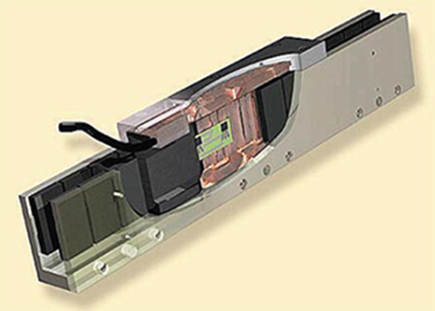
Fig. 2.24. Flat double-sided PM LBM with inner moving coil. Photo courtesy of Trilogy Systems Corporation, Webster, TX, USA.

Table 2.20. Specifications of three-phase armature propulsion winding of SC LSM on Yamanashi Maglev Test Line

Images

Panel type windings are produced in the on-site manufacturing yards. Coils are attached to the side of the reinforced concrete panel. The panel is attached to the cast-in-place concrete side walls with the aid of bolts. This type is applied to elevated bridges and high-speed sections.

A side-wall beam shown in Fig. 2.25 is a box-type girder. Styrofoam is embedded in the hollow box-type beam to reduce the mass and facilitate the construction. Ground coils are attached to the beam in the manufacturing yard. The beam is then transported to the site and erected on the preproduced support. This type is also applied to elevated bridges and high-speed sections.

In the direct attachment type guideway, the coils of the winding are attached direct to the side wall of a cast-in-place reinforced concrete structure. This type, unlike the panel or side-wall beam type, cannot respond to structural displacements [241]. The direct attachment guidaway is applied mainly to tunnel sections situated on solid ground.

Images

Fig. 2.25. Side-wall beam-type guideway of the Yamansahi Maglev Test Line: 1 — armature (propulsion) winding, 2 — levitation and guidance coil, 3 — twin beams. Courtesy of Central Japan Railway Company and Railway Technical Research Institute, Tokyo, Japan.

The resistance of the slotless armature winding can be calculated using eqn (2.29). It is recommended that the finite element method (FEM) be used for calculating the inductance.

2.11 Electromagnetic Excitation Systems

Electromagnetic excitation systems, i.e., salient ferromagnetic poles with d.c. winding, are used in large-power LSMs. For example, the German Transrapid system has on board mounted electromagnets (Fig. 2.26), which are used both for propulsion (excitation system of the LSM) and electromagnetic (EML) levitation (attraction forces). Electromagnet modules are approximately 3-m long [234]. There are 12 poles per one module. To deliver electric power to the vehicle, linear generator windings are integrated with each excitation pole. Electromagnet modules are fixed to the levitation frame with the aid of maintenance-free joints. The necessary freedom of movement is obtained by the use of vibration-damping elastic bearings.

Images

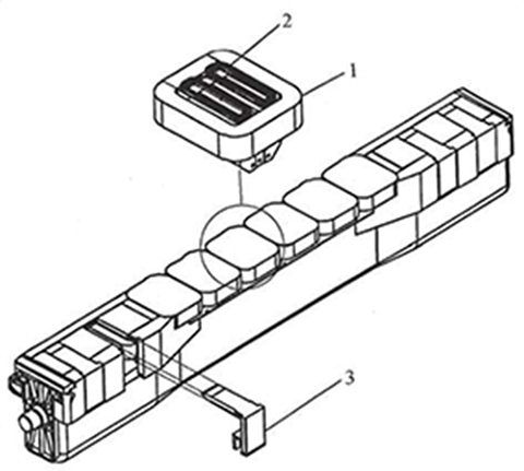
Fig. 2.26. Electromagnetic excitation system with salient poles of Transrapid maglev vehicle: 1 — d.c. excitation winding, 2 — linear generator winding, 3 — air gap sensor. Courtesy of Thyssen Transrapid System, München, Germany.

Images

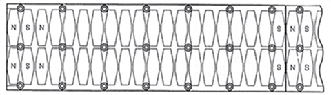
Fig. 2.27. Hexagonal assembly of PMs of LBM. Courtesy of Anorad Corporation, Hauppauge, NY, USA.

2.12 Permanent Magnet Excitation Systems

To minimize the thrust ripple in LSMs or LBMs with slotted armature stack, PMs need to be skewed. The skew is approximately equal to one tooth pitch of the armature — eqn (2.28). Instead of skewed assembly (Fig. 1.9) of rectangular PMs, Anorad Corporation proposes to use hexagonal PMs, the symmetry axis of which is perpendicular to the direction of motion (Fig. 2.27) [12].

There are practically no power losses in PM excitation systems (except higher harmonic losses), which do not require any forced cooling or heat exchangers.

2.13 Superconducting Excitation Systems

Table 2.21. Specifications of SC electromagnet of MLX01 vehicle

Images

Fig. 2.28. MLX01 SC electromagnet and bogie frame. 1 — SC electromagnet, 2 — tank, 3 — bogie frame. Courtesy of Central Japan Railway Company and Railway Technical Research Institute, Tokyo, Japan.

Superconducting (SC) excitation systems are recommended for high power LSMs which can be used in high speed ELD levitation transport.

In 1972, an experimental SC maglev test vehicle ML100 was built in Japan. Since 1977, when the Miyazaki Maglev Test Center on Kyushu Island opened, maglev vehicles ML and MLU with SC LSMs and electrodynamic suspension systems have been systematically tested. Air-cored armature winding has been installed in the form of a guideway on the ground. In 1990, a new 18.4 km Yamanashi Maglev Test Line (near Mount Fuji) for electrodynamic levitation vehicles with SC LSMs was constructed. In 1993, a test run of MLU002N (Miyazaki) started and since 1995 vehicles MLX01 (Yamanashi Maglev Test Line) have been tested.

Images

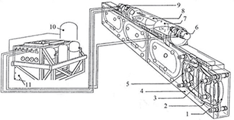
Fig. 2.29. Structure of the MLX01 SC electromagnet and on-board refrigeration system: 1 — SC winding (inner vessel), 2 — radiation shield plate, 3 — support, 4 — outer vessel, 5 — cooling pipe, 6 — 80 K refrigerator, 7 — liquid nitrogen reservoir, 8 — liquid helium reservoir, 9 — 4 K refrigerator, 10 — gaseous helium buffer tank, 11 — compressor unit. Courtesy of Central Japan Railway Company and Railway Technical Research Institute, Tokyo, Japan.

Fig. 2.28 shows the bogie frame and Fig. 2.29 shows the structure of the LTS electromagnet of the MLX01 vehicle manufactured by Toshiba, Hitachi, and Mitsubishi. The bogie frame (Sumitomo Heavy Industries) is laid under the vehicle body. The LTS electromagnet (Table 2.21) is wound with a BSCCO wire and enclosed by and integrated with a stainless inner vessel (Fig. 2.29). The winding is made of niobium—titanium alloy wire, which is embedded in a copper matrix in order to improve the stability of superconductivity. Permanent flow of current without losses is achieved by keeping the coils within a cryogenic temperature (4.2 K or −269⁰C) using liquid helium. The inner vessel is covered with a radiation shield plate on which a cooling pipe is crawled and liquid nitrogen is circulated inside the pipe to eliminate radiation heat [224]. The shield plate is kept at liquid nitrogen temperature, the boiling point of which is about 77 K.

These components are covered with an outer aluminum vacuum vessel (room temperature) and an insulating material that is packed in the space between the inner vessel and outer vessel [224]. The space is maintained in a high-vacuum range to prolong the life of the insulation. There are four sets of inner vessels (LTS electromagnet) per one outer vessel. The on-board 4 K Gifford–McMahon/Joule–Thomson refrigerator for helium, 80 K Gifford– McMahon refrigerator for nitrogen, liquid helium reservoir, and liquid nitrogen reservoir are incorporated inside the tank on the top of the outer vessel. This refrigerator reliquefies the helium gas evaporated as a result of heat generation inside the LTS electromagnet. For commercial use, electromagnets should be operated with no supply of both liquid helium and liquid nitrogen. The necessary equipment such as the compressor, which supplies the compressed gas to the helium refrigerator and control units for the operation of LTS electromagnets, are located inside the bogie.

Images

Fig. 2.30. PM HLSM. 1 — forcer, 2 — platen, 3 — mechanical or air bearing, 4 — umbilical cable with power and air hose. Courtesy of Normag Northern Magnetics Inc., Santa Clarita, CA, USA.

Images

Fig. 2.31. Longitudinal sections of forcers of HLSMs: (a) symmetrical forcer, (b) asymmetrical forcer.

2.14 Hybrid Linear Stepping Motors

The PM HLSM manufactured by Normag Northern Magnetics, Inc., Santa Clarita, CA, USA is shown in Fig. 2.30 [161].

Magnetic circuits of forcers of HLSMs are made of high permeable elec-trotechnical steels. The thickness of lamination is about 0.2 mm as the input frequency is high. Forcers are designed as symmetrical, i.e., with the PM joining the two stacks (Fig. 2.31a) or two PMs (Fig. 1.19) or asymmetrical, i.e., with PM located in one stack (Fig. 2.31b) designs. The asymmetrical design is easier for assembly.

Examples

Example 2.1

An LSM rated at 60 Hz input frequency is fed from a 50 Hz power supply at the same voltage. Losses in the armature teeth at 60 Hz are ΔP_{F et60} = 420 W and losses in the armature core (yoke) are ΔP_{F ec60} = 310 W. The hysteresis losses amount to 75% of the total core losses. Find the hysteresis, eddy current and total losses in the armature core at 50 Hz.

Solution

Hysteresis losses in armature teeth at 60 Hz

Δ P h t 60 = 0.75 Δ P F e t 60 = 0.75 \times 420 = 315 W

$Δ P_{h t 60} = 0.75 Δ P_{F e t 60} = 0.75 \times 420 = 315 W$

Hysteresis losses in armature core (yoke) at 60 Hz

Δ P h c 60 = 0.75 Δ P F e c 60 = 0.75 \times 310 = 232.5 W

$Δ P_{h c 60} = 0.75 Δ P_{F e c 60} = 0.75 \times 310 = 232.5 W$

Total hysteresis losses at 60 Hz

Δ P h 60 = Δ P h t 60 + Δ P h c 60 = 315 + 232.5 = 547.5 W

$Δ P_{h 60} = Δ P_{h t 60} + Δ P_{h c 60} = 315 + 232.5 = 547.5 W$

The magnetic flux density is proportional to the EMF, which in turn is proportional to the frequency. Therefore, the magnetic flux density at 60 Hz magnetic flux density at 50 Hz ratio is

b = f 60 f 50 = 60 50 = 1.2

$b = \frac{f_{60}}{f_{50}} = \frac{60}{50} = 1.2$

On the basis of eqn (2.2) hysteresis losses in teeth at 50 Hz are

Δ P h t 50 = f 50 f 60 b 2 Δ P h t 60 = 50 60 \times 1.2 2 \times 315 = 378 W

$Δ P_{h t 50} = \frac{f_{50}}{f_{60}} b^{2} Δ P_{h t 60} = \frac{50}{60} \times {1.2}^{2} \times 315 = 378 W$

Hysteresis losses in armature core at 50 Hz are

Δ P h c 50 = f 50 f 60 b 2 Δ P h c 60 = 50 60 \times 1.2 2 \times 232.5 = 279 W

$Δ P_{h c 50} = \frac{f_{50}}{f_{60}} b^{2} Δ P_{h c 60} = \frac{50}{60} \times {1.2}^{2} \times 232.5 = 279 W$

Total hysteresis losses at 50 Hz

Δ P h 50 = Δ P h t 50 + Δ P h c 50 = 378 + 279 = 657 W

$Δ P_{h 50} = Δ P_{h t 50} + Δ P_{h c 50} = 378 + 279 = 657 W$

Eddy-current losses in armature teeth at 60 Hz

Δ P e t 60 = Δ P F e t 60 - Δ P h t 60 = 420 - 315 = 105 W

$Δ P_{e t 60} = Δ P_{F e t 60} - Δ P_{h t 60} = 420 - 315 = 105 W$

Eddy-current losses in armature core (yoke) at 60 Hz

Δ P e c 60 = Δ P F e c 60 - Δ P h c 60 = 310 - 232.5 = 77.5 W

$Δ P_{e c 60} = Δ P_{F e c 60} - Δ P_{h c 60} = 310 - 232.5 = 77.5 W$

Total eddy-current losses at 60 Hz

Δ P e 60 = Δ P e t 60 + Δ P e c 60 = 105 + 77.5 = 182.5 W

$Δ P_{e 60} = Δ P_{e t 60} + Δ P_{e c 60} = 105 + 77.5 = 182.5 W$

On the basis of eqn (2.2), eddy-current losses in armature teeth at 50 Hz are

Δ P e t 50 = (f 50 f 60) 2 b 2 Δ P e t 60 = (50 60) 2 \times 1.2 2 \times 105 = 105 W

$Δ P_{e t 50} = {(\frac{f_{50}}{f_{60}})}^{2} b^{2} Δ P_{e t 60} = {(\frac{50}{60})}^{2} \times {1.2}^{2} \times 105 = 105 W$

Eddy-current losses in armature core at 50 Hz are

Δ P e c 50 = (f 50 f 60) 2 b 2 Δ P e t 60 = (50 60) 2 \times 1.2 2 \times 77.5 = 77.5 W

$Δ P_{e c 50} = {(\frac{f_{50}}{f_{60}})}^{2} b^{2} Δ P_{e t 60} = {(\frac{50}{60})}^{2} \times {1.2}^{2} \times 77.5 = 77.5 W$

Total eddy-current losses at 50 Hz

Δ P e 50 = Δ P e t 50 + Δ P e c 50 = 105 + 77.5 = 182.5 W

$Δ P_{e 50} = Δ P_{e t 50} + Δ P_{e c 50} = 105 + 77.5 = 182.5 W$

If the frequency is reduced from 60 to 50 Hz, hysteresis losses increase while eddy-current losses remain the same.

Total losses in the armature stack at 60 Hz

Δ P F e 60 = Δ P h 60 + Δ P e 60 = 547.5 + 182.5 = 730 W

$Δ P_{F e 60} = Δ P_{h 60} + Δ P_{e 60} = 547.5 + 182.5 = 730 W$

Total losses in the armature stack at 50 Hz

Δ P F e 50 = Δ P h 50 + Δ P e 50 = 657 + 182.5 = 839.5 W

$Δ P_{F e 50} = Δ P_{h 50} + Δ P_{e 50} = 657 + 182.5 = 839.5 W$

If the frequency is reduced form 60 to 50 Hz, the total losses in the armature stack increase, i.e.,

Δ P F e 50 Δ P F e 50 = 839.5 730 = 1.15

$\frac{Δ P_{F e 50}}{Δ P_{F e 50}} = \frac{839.5}{730} = 1.15$

because the magnetic flux density at the same number of turns and voltage increases as the frequency decreases.

Example 2.2

Find the losses in the armature core of a single-sided 6-pole, 18-slot, 100-Hz, 3-phase PM LSM. The dimensions of the armature core are as follows:

pole pitch τ = 48.0 mm
coil pitch w_c = 48.0 mm
effective length of armature stack L_i = 96.0 mm
height of primary core (yoke) h_1c = 10.0 mm
armature tooth width c_t = 7.0 mm
armature tooth height h_t = 23.5 mm
armature tooth width c_t = 9.0 mm
armature slot opening b₁₄ = 3.0 mm

The magnetic flux density in armature teeth is B_1t = 1.678 T, flux density in the armature core (yoke) B_1c = 1.468, specific core losses at 50 Hz and 1 T are Δp_1/50 = 1.07 W/kg, stacking factor k_i = 0.96, and the factors in eqn (2.3) accounting for the increase in losses due to metallurgical and manufacturing processes are k_adt = 1.6 and k_adc = 3.2.

Solution

Slot pitch according to eqn (2.28)

t 1 = 9.0 + 8.0 = 16 mm

$t_{1} = 9.0 + 8.0 = 16 mm$

Number of slots half-filled with armature winding according to eqn (2.9)

s' 1 = 1 6 (6 + 48.0 48.0) \times 18 = 21

${s^{'}}_{1} = \frac{1}{6} (6 + \frac{48.0}{48.0}) \times 18 = 21$

Length of stack with half-filled slots

L s t a c k = s' 1 t 1 + c t = 21 \times 0.016 + 0.007 = 0.343 / m

$L_{s t a c k} = {s^{'}}_{1} t_{1} + c_{t} = 21 \times 0.016 + 0.007 = 0.343 / m$

Mass of armature teeth

m 1 t = 7800 (s' 1 + 1) c t h t L i k i = 7800 (21 + 1) \times 0.007 \times 0.0235 \times 0.096 \times 0.96 = 2.60 kg

$m_{1 t} = 7800 ({s^{'}}_{1} + 1) c_{t} h_{t} L_{i} k_{i} = 7800 (21 + 1) \times 0.007 \times 0.0235 \times 0.096 \times 0.96 = 2.60 kg$

Mass of armature core (yoke)

m 1 c = 7800 L s t a c k h 1 c L i k i = 7800 \times 0.343 \times 0.01 \times 0.096 \times 0.96 = 2.47 kg

$m_{1 c} = 7800 L_{s t a c k} h_{1 c} L_{i} k_{i} = 7800 \times 0.343 \times 0.01 \times 0.096 \times 0.96 = 2.47 kg$

Core losses at f = 100 Hz calculated according to eqn (2.3)

Δ P F e = 1.07 (100 50) 4 / 3 (1.6 \times 1.678 2 \times 2.60 + 3.2 \times 1.468 2 \times 2.47) = 77.4 W

$Δ P_{F e} = 1.07 {(\frac{100}{50})}^{4 / 3} (1.6 \times {1.678}^{2} \times 2.60 + 3.2 \times {1.468}^{2} \times 2.47) = 77.4 W$

Example 2.3

Find the operating point of an NdFeB grade N35H PM with rectangular cross section placed in a mild steel magnetic circuit with air gap. The parameters of the PM are

remanent magnetic flux desnity at 20° C B_r20 = 1.18 T
coercive force at 20° C H_c20 = 900 kA/m
temperature coefficeint for B_r α_B = −0.11 %/°C
temperature coefficeint for H_c α_H = −0.45 %/^o°C

The PM temperature is θ = 100 °C; the dimensions of PM are w_M = 42 mm, l_M = 105 mm, h_M = 5.0 mm; the air gap is g = 1.6 mm, and the PM leakage flux coefficient is σ_lM = 1.2.

Solution

Remanence and coercivity at θ = 100 °C according to eqns (2.21) and (2.22)

B r = 1.18 [1 + - 0.11 100 (100 - 20)] = 1.076 T H c = 900 [1 + - 0.45 100 (100 - 20)] = 576 kA / m

$\begin{matrix} B_{r} = 1.18 [1 + \frac{- 0.11}{100} (100 - 20)] = 1.076 T \\ H_{c} = 900 [1 + \frac{- 0.45}{100} (100 - 20)] = 576 kA / m \end{matrix}$

Relative recoil magnetic permeability

μ r r e c = 1.076 0.4 π \times 10 - 6 \times 576000 = 1.487

$μ_{r r e c} = \frac{1.076}{0.4 π \times 10^{- 6} \times 576000} = 1.487$

Equivalent air gap

g e q = g + h M μ r r e c = 1.6 + 5.0 1.487 = 4.96 mm

$g_{e q} = g + \frac{h_{M}}{μ_{r r e c}} = 1.6 + \frac{5.0}{1.487} = 4.96 mm$

Permeance of the air gap according to eqn (B.2)

G g = 0.4 π \times 10 - 6 0.042 \times 0.105 0.00496 = 1.117 \times 10 - 7 H

$G_{g} = 0.4 π \times 10^{- 6} \frac{0.042 \times 0.105}{0.00496} = 1.117 \times 10^{- 7} H$

Permeance for total magnetic flux

G t = μ 0 w M l M g e q σ l M = 0.4 π \times 10 - 6 0.042 \times 0.105 0.00496 \times 1.2 = 1.340 \times 10 - 7 H

$G_{t} = μ_{0} \frac{w_{M} l_{M}}{g_{e q}} σ_{l M} = 0.4 π \times 10^{- 6} \frac{0.042 \times 0.105}{0.00496} \times 1.2 = 1.340 \times 10^{- 7} H$

Line representing the total permeance, which intersects the demagnetization curve (Fig. 2.32)

Images

Fig. 2.32. Operating point (B_g = 0.608 T, H_t = 185 694.5 A/m) of PM on demagnetization curve. Numerical example 2.3.

B t (H) = μ 0 h M g H T

$\begin{matrix} B_{t} (H) = μ_{0} \frac{h_{M}}{g} H & T \end{matrix}$

Magnetic field intensity corresponding to B_t

H t = B r μ 0 h M / g + B r / H c = 1.076 0.4 π \times 10 - 6 \times 0.005 / 0.0016 + 1.076 / 576000 = 185694.5 A / m

$\begin{matrix} H_{t} = \frac{B_{r}}{μ_{0} h_{M} / g + B_{r} / H_{c}} \\ = \frac{1.076}{0.4 π \times 10^{- 6} \times 0.005 / 0.0016 + 1.076 / 576000} = 185694.5 A / m \end{matrix}$

For H_t = 185 694.5 A/m, the corresponding magnetic flux density B_t = 0.729 T. The air gap magnetic flux density as obtained from the PM diagram (Fig. 2.32)

B g = B r (1 - H t H c) 1 σ l M = 1.076 (1 - 185694.5 576000) 1 1.2 = 0.608 T

$B_{g} = B_{r} (1 - \frac{H_{t}}{H_{c}}) \frac{1}{σ_{l M}} = 1.076 (1 - \frac{185694.5}{576000}) \frac{1}{1.2} = 0.608 T$

This point (B_g = 0.608 T, H_t = 185 694.5 A/m) is the intersection point of the demagnetization curve B(H) and permeance line B_t(H) in Fig. 2.32. The air gap magnetic flux

Φ g = B g w M l M = 0.608 \times 0.042 \times 0.105 = 0.00268 Wb

$Φ_{g} = B_{g} w_{M} l_{M} = 0.608 \times 0.042 \times 0.105 = 0.00268 Wb$

Example 2.4

Given below are dimensions of the armature core of a single-sided 6-pole, 18-slot, 50-Hz, 3-phase PM LSM with semiopen slots (Fig. 2.17a:

pole pitch τ = 48.0 mm
effective length of armature stack L_i = 96.0 mm
dimensions of PM: h_M = 3.0 mm, w_M = 40.0 mm, l_M = 96.0 mm
height of primary core (yoke) h_1c = 10.0 mm
height of reaction rail core (yoke) h_2c = 12.0 mm
armature tooth width c_t = 8.0 mm
armature tooth height h_t = 23.5 mm
armature slot vertical dimensions h₁₁ = 20 mm, h₁₂ = 1.0 mm, h₁₃ = 2.0 mm, h₁₄ = 0.5 mm
armature slot width b₁₁ = 8.0 mm
armature slot opening b₁₄ = 3.0 mm
air gap (mechanical clearance) g = 1.5 mm

The number of turns per phase is N₁ = 180, the coil pitch is equal to the slot pitch (w_c = τ), the armature core stacking factor k_i = 0.96, the skin effect coefficient for reactance k_1X ≈ 1.0, and the armature slots are unskewed. The saturation factor of magnetic circuit is k_sat = 1.153.

Find the stator winding leakage reactance X₁.

Solution

The number of slots per pole is Q₁ = 18/6 = 3, number of slots per pole per phase q₁ = 18/(3×6) = 1, winding distribution factor k_d1 = sin[π/(2×3)]/(1× sin[π/(2×3×1)] = 1, winding pitch factor k_p1×0.048/(2×0.048)] = 1, winding factor k_w1 = 1 × 1 = 1, and slot pitch t₁ = c_t + b₁₁ = 8.0 + 8.0 = 16 mm.

The coefficient of leakage permeance for semi-open slot according to eqn (2.33)

λ 1 s = 20.0 3 \times 8.0 + 1.0 8.0 + 2 \times 2.0 8.0 + 3.0 + 0.5 3.0 = 1.489

$λ_{1 s} = \frac{20.0}{3 \times 8.0} + \frac{1.0}{8.0} + \frac{2 \times 2.0}{8.0 + 3.0} + \frac{0.5}{3.0} = 1.489$

Estimated length of single-sided end turn

l 1 e = 1.3 τ + 0.004 = 1.3 \times 0.048 + 0.004 = 0.066 m

$l_{1 e} = 1.3 τ + 0.004 = 1.3 \times 0.048 + 0.004 = 0.066 m$

The coefficient of leakage permeance for end turns according to eqn (2.36)

λ 1 e = 0.34 \times 1.0 (1 - 2 π 0.048 0.066) = 0.184

$λ_{1 e} = 0.34 \times 1.0 (1 - \frac{2}{π} \frac{0.048}{0.066}) = 0.184$

where w_c = τ = 0.048 m. The armature winding differential leakage factor calculated according to eqn (2.46) for ν = 2000 is τ_d1 = 0.096456. This coefficient can also be calculated on the basis of simplified formula (2.47), i.e.,

τ d 1 = π 2 ( 10 \times 1.0 2 + 2 ) 27 [sin(30 o 1.0)] 2 - 1 = 0.09662

$τ_{d 1} = \frac{π^{2} (10 \times {1.0}^{2} + 2)}{27} {[sin(\frac{30^{o}}{1.0})]}^{2} - 1 = 0.09662$

Carter’s coefficient according to eqn (2.44)

k C 1 = 0. \cdot 016 0.016 - 05587 \times 0.016 = 1.0553

$k_{C 1} = \frac{0. \cdot 016}{0.016 - 05587 \times 0.016} = 1.0553$

where γ₁ = 0.5587 has been obtained from eqn (2.45). The specific permeance for differential leakage flux according to eqn (2.43)

λ 1 d = 3 \times 1 \times 0.048 \times 1.0 2 π 2 \times 0.0015 \times 1.0553 \times 1.153 0.096456 = 0.771

$λ_{1 d} = \frac{3 \times 1 \times 0.048 \times {1.0}^{2}}{π^{2} \times 0.0015 \times 1.0553 \times 1.153} 0.096456 = 0.771$

The coefficient of tooth-top permeance according to eqn (2.51)

λ 1 t = 5 \times 1.5 / 3.0 5 + 4 \times 1.5 / 3.0 = 0.357

$λ_{1 t} = \frac{5 \times 1.5 / 3.0}{5 + 4 \times 1.5 / 3.0} = 0.357$

Leakage reactance of the armature winding according to eqn (2.32) in which k_1X = 1.0

X 1 = 4 π \times 50 \times 0.4 π \times 10 - 6 0.096 \times 180 2 3 \times 1 (1.489 \times 1.0 + 0.066 0.096 0.184 + 0.771 + 0.357) = 2.246 Ω

$\begin{matrix} X_{1} = 4 π \times 50 \times 0.4 π \times 10^{- 6} \frac{0.096 \times 180^{2}}{3 \times 1} (1.489 \times 1.0 + \frac{0.066}{0.096} 0.184 + 0.771 + 0.357) \\ = 2.246 Ω \end{matrix}$

^¹METGLAS® is a registered trademark of AlliedSignal, Inc.

^²Quenching is a resistive heating of an SC and a sudden temperature rise.

^³Perovskite (In German “Perovskit”) was discovered in the Ural mountains of Russia by G. Rose in 1839 and named for Russian mineralogist, L. A. Perovski (1792—1856).

^⁴Deposition (in chemistry) is the settling of particles (atoms or molecules) or sediment from a solution, suspension mixture, or vapor onto a preexisting surface.

^⁵Texture in materials science is the distribution of crystallographic orientations of a sample. Biaxially textured means textured along two axes.

..................Content has been hidden....................

You can't read the all page of ebook, please click here login for view all page.

Table of Contents for
2 Materials and Construction

2

Materials and Construction

2.1 Materials

2.2 Laminated Ferromagnetic Cores

2.2.1 Electrical Sheet-Steels

2.2.2 High-Saturation Ferromagnetic Alloys

2.2.3 Permalloys

2.2.4 Amorphous Materials

2.2.5 Solid Ferromagnetic Materials

2.2.6 Soft Magnetic Powder Composites

2.3 Permanent Magnets

2.3.1 Demagnetization Curve

2.3.2 Magnetic Parameters

2.3.3 Magnetic Flux Density in the Air Gap

2.3.4 Properties of Permanent Magnets

2.4 Conductors

2.4.1 Magnet Wire

2.4.2 Resistivity and Conductivity

2.5 Insulation Materials

2.5.1 Classes of Insulation

2.5.2 Commonly Used Insulating Materials

2.5.3 Impregnation

2.6 Principles of Superconductivity

2.7 Superconducting Wires

2.7.1 Classification of HTS Wires

2.7.2 HTS Wires Manufactured by American Superconductors

2.7.3 HTS Wires Manufactured by SuperPower

2.8 Laminated Stacks

2.9 Armature Windings of Slotted Cores

2.10 Slotless Armature Systems

2.11 Electromagnetic Excitation Systems

2.12 Permanent Magnet Excitation Systems

2.13 Superconducting Excitation Systems

2.14 Hybrid Linear Stepping Motors

Examples

Table of Contents for 2 Materials and Construction

Create new playlist

Sign In

Sign Up

Table of Contents for
2 Materials and Construction