Appendix D Field-Network Simulation of Dynamic Characteristics of PM LSMs

Search in book...
Toggle Font Controls
Create new playlist

Name your new playlist

Playlist description (optional)
Sign In

Email address

Password

Forgot Password?

or

Continue with Facebook

Continue with Google
Sign Up

Full Name

Email address

Confirm Email Address

Password

or

Continue with Facebook

Continue with Google

In order to understand the behavior of an electromagnetic system, it is important to comprehend the dynamics of its components.

There are several basic methods of formulating the equations of motion and thereby obtaining the characteristics of the electromagnetic energy conversion devices. These are through the applications of [145, 238]

electromagnetic field theory;
principle of virtual work;
variational principles.

Each of the above approaches has its own merits and, in some cases, one cannot be conveniently substituted by the other [209, 225].

Mechanical and electrical parameters of the system are necessary to formulate the equations of motion. Electrical parameters can be evaluated on the basis of electromagnetic field theory. In most cases, such as tubular PM LSMs operating at power frequencies, the electric field distribution is not of importance, and only the magnetic field must be analyzed.

Images

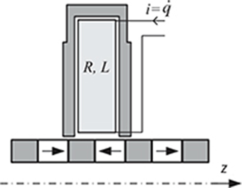
Fig. D.1 A segment of a tubular PM LSM for transient analysis.

In [218] the so-called field-network model has been obtained on the basis of the Lagrange function [238]. The tubular PM LSM has been divided into segments (modules). The symmetry axes of neighboring teeth are remote from each other by the distance equal to one pole pitch. Since each segment is magnetically separated, it can be modeled independently. Generalized coordinates ξ for one segment (Fig. D.1) are the position z of the reaction rail and the electric charge q. The Lagrangian (1.33) of a mechanical system can also be expressed with the aid of kinetic coenergy¹ E k and potential energy E_p, i.e.,

L = {E^{'}}_{k} - E_{p} (D.1)

$L = {E^{'}}_{k} - E_{p} (D.1)$

Assuming that the net potential energy E_p = 0, the kinetic coenergy E′_k of the system is

{E^{'}}_{k} = \frac{1}{2} m {\dot{z}}^{2} + \int_{0}^{\dot{q}} Ψ (\dot{\tilde{q}}, z) d \dot{\tilde{q}} (D.2)

${E^{'}}_{k} = \frac{1}{2} m {\dot{z}}^{2} + \int_{0}^{\dot{q}} Ψ (\dot{\tilde{q}}, z) d \dot{\tilde{q}} (D.2)$

Using Hamilton’s principle [145, 238], the Lagrangian (D.1) of the system is [210, 208]

L = {E^{'}}_{k} - 0 = \frac{1}{2} m {\dot{z}}^{2} + \int_{0}^{\dot{q}} Ψ (\dot{\tilde{q}}, z) d \dot{\tilde{q}} (D.3)

$L = {E^{'}}_{k} - 0 = \frac{1}{2} m {\dot{z}}^{2} + \int_{0}^{\dot{q}} Ψ (\dot{\tilde{q}}, z) d \dot{\tilde{q}} (D.3)$

Euler–Lagrange differential equation (1.36) gives two differential equations, one for electrical part and another for mechanical part of the system, i.e.,

electrical balance equation

$υ (t) = L (z, i) \frac{\partial i}{\partial t} + \frac{\partial Ψ (z, i)}{\partial z} \frac{\partial z}{\partial t} + R i (D.4)$ $υ (t) = L (z, i) \frac{\partial i}{\partial t} + \frac{\partial Ψ (z, i)}{\partial z} \frac{\partial z}{\partial t} + R i (D.4)$
mechanical balance equation

$m \frac{d^{2} z}{d t^{2}} + D_{υ} \frac{d z}{d t} = F (z, i) (D.5)$ $m \frac{d^{2} z}{d t^{2}} + D_{υ} \frac{d z}{d t} = F (z, i) (D.5)$

in which m is the mass of the reaction rail including load, D_v is the viscous friction constant, F (z, i) is the electromagnetic force developed by the tubular PM LSM, v(t) is the supply voltage, L(z, i) is the inductance of the stationary coil, Ψ(z, i) is the magnetic flux linked with the stationary coil, and R is the resistance of the coil. In the case of current excitation, eqn (D.4) can be neglected.

The Matlab/Simulink model for solving eqns (D.4) and (D.5) is presented in Fig. D.2. Mechanical characteristic f(z, i) for each phase has been implemented. Static and kinetic friction losses in the linear slide bearings have also been taken into account. The magnetization curve B–H has been included in eqn (D.4).

Images

Fig. d.2 Circuit diagram for Matlab/Simulink simulation.

The field-network model performs the calculation of the dynamics of the tubular PM LSM (Fig. 5.14) fed from a sinusoidal source. Since the magnetic circuit is nonlinear, a direct solution to eqn (D.4) is almost impossible. Thus, after finding the integral parameters of the electromagnetic field, the combined mechanical balance and electric field equations have been solved simultaneously. Some calculated and measured values of the position of the reaction rail versus time are plotted in Figs. D.3 to D.5.

In computer simulations, the position of the reaction rail varies from z(t) = 0 to |z(t)| = 0.1 m, mass of reaction rail m = 1.3 kg, μ_v = 50 Ns/m, R = 1.6 Ω, and I_a = 8 A. No-load operating conditions have been assumed. The average velocity of the reaction rail v = 1000 mm/s.

Experimental verification of the reaction rail movement has also been performed for the tubular PM LSM under load. Simulation results of the reaction rail movement have been verified experimentally for loaded tubular PM LSM. The load force has been created by an additional mass rigidly connected and moving with the reaction rail. For the mass m = 3.2 kg, the position of the reaction rail versus time is shown in Fig. D.4 and for the mass m = 19.2 kg, the same plot is shown in Fig. D.5. Test results (Figs D.4 and D.5) are in good agreement with the calculations.

Images

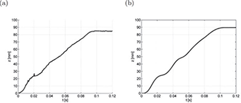
Fig. D.3 Position of reaction rail versus time at v = 1000 mm/s: (a) test results, (b) calculations.

Images

Fig. D.4 Position of reaction rail versus time at average velocity v = 50 mm/s and inertial mass m = 3.2 kg: (a) test results, (b) calculations.

Images

Fig. D.5 Position of reaction rail versus time at average velocity v = 50 mm/s and inertial mass m = 19.2 kg: (a) test results, (b) calculations.

Images

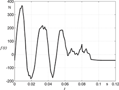
Fig. D.6 Computed electromagnetic force versus time at no load and v = 1000 mm/s.

Images

Fig. D.7 Electromagnetic force versus time at average velocity v = 50 mm/s and inertial mass m = 3.2 kg.

Images

Fig. D.8 Electromagnetic force versus time at average velocity v = 50 mm/s and inertial mass m = 19.2 kg.

The simulation of the waveform of the electromagnetic force has been performed at no-load and nominal speed (Fig. D.6). The peak value of the electromagnetic force is 360 N. There are only a few oscillations of the electromagnetic force. At reduced velocity of the reaction rail, the force ripple increases (Figs D.7 and D.8). It can be observed that the peak force is a nonlinear function of the load mass. If the load mass increases six times, the electromagnetic force increases only twice.

^¹Coenergy (a second state function of the energy) is an auxiliary function necessary for calculations of the force or torque at constant current.

..................Content has been hidden....................

You can't read the all page of ebook, please click here login for view all page.

Table of Contents for Appendix D Field-Network Simulation of Dynamic Characteristics of PM LSMs

Create new playlist

Sign In

Sign Up

Appendix D

Field-Network Simulation of Dynamic Characteristics of PM LSMs

Table of Contents for
Appendix D Field-Network Simulation of Dynamic Characteristics of PM LSMs