10 Industrial Automation Systems

Search in book...
Toggle Font Controls
Create new playlist

Name your new playlist

Playlist description (optional)
Sign In

Email address

Password

Forgot Password?

or

Continue with Facebook

Continue with Google
Sign Up

Full Name

Email address

Confirm Email Address

Password

or

Continue with Facebook

Continue with Google

Manufacturing processes can be classified as follows [49]:

Casting, foundry or molding processes
Forming or metalworking processes
Machining (material removal) processes
Joining (fastening, welding, fitting, bonding) and assembly
Surface treatments and finishing (cleaning, tumbling, scribing, polishing, coating, plating)
Heat treating
Other, e.g., inspection, testing, packaging, storing, etc.

Manufacturing process automation frees the human operator from control functions, i.e., from the need to perform certain actions in a particular sequence to carry out an operation in accord with preset machining conditions.

Automation is the use of the energy of a nonliving system to control and carry out a process or process operation without direct human intervention [200]. The object of automation is to make the best use of available resources, materials, and machines. The human worker’s function is limited to machine supervisory control and elimination of possible deviations from the prescribed process (corrective adjustment).

According to the Yardstick for Automation chart (Table 10.1) presented by G.H. Amber and P.S. Amber in 1962 [8], each level of automation is tied to a human attribute that is being replaced by the machine. Thus the A(0) level of automation, in which no human attribute was mechanized, covers Stone Age through Iron Age. So far, levels A(5), A(6), and A(7) have partially been implemented or are subject to intensive research. Levels A(8) and A(9) are still topics of science fiction.

In automatic systems, actuation components are adapted to moving various mechanisms of machine tools to execute the required step of control, e.g., change the mode of operation, release a workpiece, start or stop the machine, etc. One of the emerging technologies is the use of linear motors as electrical actuators.

Table 10.1. Yardstick for Automation [8].

Images

10.2 Ball Lead Screws

10.2.1 Basic Parameters

Normally, the rotation of a rotary servo motor, usually PM brushless motor, is converted into linear motion in x, y, z, or w (e.g., tool) direction with the aid of ball lead screws (Fig. 10.1).

For a screw of mean diameter d, the helix angle Θ is given by the equation

\tan (Θ) = \frac{l}{π d} = \frac{2 t_{r}}{d} (10.1)

$\tan (Θ) = \frac{l}{π d} = \frac{2 t_{r}}{d} (10.1)$

where t_r is the transmission parameter (axial distance moved per one radian of screw revolution) of the lead screw. The lead l of the screw (helix) is the axial distance moved by the nut in one revolution of the screw:

Images

Fig. 10.1. Longitudinal section of a ball lead screw. 1 — table movement, 2 — recirculating ball lead screw, 3 — recirculating balls, 4 — ball nut attached to the table.

l = 2 π t_{r} (10.2)

$l = 2 π t_{r} (10.2)$

In general, the lead l is not the same as the pitch τ_l of the screw. The pitch τ_l is the axial distance between two adjacent threads (Fig. 10.1). For a screw with k independent threads on the screw shaft,

l = k τ_{l} (10.3)

$l = k τ_{l} (10.3)$

For a single start screw, k = 1 and l = τ_l. If T_b is the torque provided by the screw, i.e., net torque after subtracting the inertia torque due to inertia of the motor rotor and lead screw, the force is

F = \frac{η_{b}}{t_{r}} T_{b} = \frac{2 π η_{b}}{l} T_{b} (10.4)

$F = \frac{η_{b}}{t_{r}} T_{b} = \frac{2 π η_{b}}{l} T_{b} (10.4)$

where η_b is the efficiency of the ball screw. The frictional force

F_{f} = μ_{υ} \frac{T_{b}}{t_{r}} (10.5)

$F_{f} = μ_{υ} \frac{T_{b}}{t_{r}} (10.5)$

where the coefficient of friction μ_v = 0.2 for steel (dry), μ_v = 0.15 for steel (lubricated), μ_v = 0.1 for bronze, and μ_v = 0.1 for plastic. The torque required to overcome this frictional force is

T_{f} = F_{f} \frac{d}{2} = μ_{υ} d \frac{T_{b}}{2 t_{r}} (10.6)

$T_{f} = F_{f} \frac{d}{2} = μ_{υ} d \frac{T_{b}}{2 t_{r}} (10.6)$

The efficiency of the ball screw

η_{b} = \frac{T_{b} - T_{f}}{T_{b}} = 1 - μ_{υ} \frac{d}{2 t_{r}} = 1 - \frac{μ_{υ}}{\tan (Θ)} (10.7)

$η_{b} = \frac{T_{b} - T_{f}}{T_{b}} = 1 - μ_{υ} \frac{d}{2 t_{r}} = 1 - \frac{μ_{υ}}{\tan (Θ)} (10.7)$

The linear speed (travel rate) is the rotational speed n at which the screw or nut is rotating multiplied by the lead of the screw, i.e.,

υ = n τ_{l} (10.8)

$υ = n τ_{l} (10.8)$

10.2.2 Ball Lead Screw Drives

The force balance equation of a linear drive system can be described by the following equation:

m \frac{d^{2} x}{d t^{2}} + D_{υ} \frac{d x}{d t} + k_{s} x + F_{e x t} (t) = F_{d x} (t) (10.9)

$m \frac{d^{2} x}{d t^{2}} + D_{υ} \frac{d x}{d t} + k_{s} x + F_{e x t} (t) = F_{d x} (t) (10.9)$

where m is the total mass of the load including the table (thrust block), D_v is the viscous friction (damping) constant of the load, k_s is the spring constant, F_dx is electromagnetic force produced by the motor, F_ext represent all external (disturbance) forces acting on the system, and x is the linear displacement of the load.

The position displacement, velocity, and acceleration of a linear drive can be expressed as

x (t) = X_{m} \sin (w t) (10.10)

$x (t) = X_{m} \sin (w t) (10.10)$

\dot{x} (t) = \frac{d x (t)}{d t} = w X_{m} \cos (w t) (10.11)

$\dot{x} (t) = \frac{d x (t)}{d t} = w X_{m} \cos (w t) (10.11)$

\ddot{x} (t) = \frac{d^{2} x (t)}{d t^{2}} = - w^{2} X_{m} \sin (w t) (10.12)

$\ddot{x} (t) = \frac{d^{2} x (t)}{d t^{2}} = - w^{2} X_{m} \sin (w t) (10.12)$

where X_m is the maximum position error. Assuming in eqn (10.9) F_dx = 0 (uncontrolled system) and k_s = 0, the external (disturbance) force is

F_{e x t} = m w^{2} X_{m} \sin (w t) + D_{υ} w X_{m} \cos (w t) (10.13)

$F_{e x t} = m w^{2} X_{m} \sin (w t) + D_{υ} w X_{m} \cos (w t) (10.13)$

Neglecting the viscous friction constant (D_v ≈ 0), the external force becomes

F_{e x t} \approx m w^{2} X_{m} \sin (w t) (10.14)

$F_{e x t} \approx m w^{2} X_{m} \sin (w t) (10.14)$

The static stiffness of a linear drive system is defined as the external force-to-position displacement ratio, i.e.,

K_{s} = \frac{F_{e x t}}{x} (10.15)

$K_{s} = \frac{F_{e x t}}{x} (10.15)$

The dynamic stiffness of a linear drive system is defined as the external force-to-system response ratio, i.e.,

K_{d} = \frac{F_{e x t} (t)}{x (t)} (10.16)

$K_{d} = \frac{F_{e x t} (t)}{x (t)} (10.16)$

Putting eqns (10.10) and (10.14) into eqn (10.16), the following simplified equation for dynamic stiffness can be written,

K_{d} \approx m w^{2} (10.17)

$K_{d} \approx m w^{2} (10.17)$

For a ball screw system with rotary motor and tooth or belt gear, the equation of motion is [151]

\begin{matrix} {m_{t} + {(\frac{2 π}{τ_{l}})}^{2} [J_{b s} + {(\frac{N_{2}}{N_{1}})}^{2} J_{m}]} \ddot{x} \\ = \frac{2 π}{τ_{l}} [\frac{N_{2}}{N_{1}} (T_{d} - D_{υ m} Θ_{m}^{\cdot} - T_{e x t m})] - \frac{2 π}{τ_{l}} (D_{υ b s} Θ_{b s}^{\cdot} + T_{e x t b s}) - D_{υ t} \dot{x} - F_{e x t} \end{matrix} (10.18)

$\begin{matrix} {m_{t} + {(\frac{2 π}{τ_{l}})}^{2} [J_{b s} + {(\frac{N_{2}}{N_{1}})}^{2} J_{m}]} \ddot{x} \\ = \frac{2 π}{τ_{l}} [\frac{N_{2}}{N_{1}} (T_{d} - D_{υ m} Θ_{m}^{\cdot} - T_{e x t m})] - \frac{2 π}{τ_{l}} (D_{υ b s} Θ_{b s}^{\cdot} + T_{e x t b s}) - D_{υ t} \dot{x} - F_{e x t} \end{matrix} (10.18)$

where m_t is the mass of the moving table, τ_l is the screw pitch; J_bs and J_m are moments of inertia of the ball screw and motor, respectively; N₁ and N₂ are the number of teeth on the motor and ball screw gears, resectively; D_vt, D_vm, D_vbs are viscous friction coefficients of the table, motor and ball screw, respectively; F_ext is the external (disturbance) force on the table; T_d is the torque developed by the motor; T_extm and Textbs are external torques acting on the motor shaft and ball screw, respectively; x is the linear displacement of the load; and Θ_m, Θ_bs are angular displacements of the motor and ball screw, respectively.

Assuming T_d = 0, D_vm = 0, D_vbs = 0, D_vt, T_extm = 0, Textbs = 0 and denoting

J_{e} = J_{b s} + {(\frac{N_{2}}{N_{1}})}^{2} J_{m} (10.19)

$J_{e} = J_{b s} + {(\frac{N_{2}}{N_{1}})}^{2} J_{m} (10.19)$

the external (disturbance) force of a ball screw system obtained from eqn (10.18) is

F_{e x t} \approx [m_{t} + {(\frac{2 π}{τ_{l}})}^{2} J_{e}] w^{2} X_{m} \sin (w t) (10.20)

$F_{e x t} \approx [m_{t} + {(\frac{2 π}{τ_{l}})}^{2} J_{e}] w^{2} X_{m} \sin (w t) (10.20)$

and dynamic stiffness

\begin{matrix} K_{d} \approx [m_{t} + {(\frac{2 π}{τ_{l}})}^{2} J_{e}] w^{2} & N / m \end{matrix} (10.21)

$\begin{matrix} K_{d} \approx [m_{t} + {(\frac{2 π}{τ_{l}})}^{2} J_{e}] w^{2} & N / m \end{matrix} (10.21)$

where J_e is the equivalent moment of inertia of the balls screw and motor. The acceleration can be found from eqns (10.4), (10.12) and (10.20), i.e.,

\begin{matrix} a \approx \frac{F_{e x t}}{m_{t} + m_{t} {(\frac{2 π}{τ_{l}})}^{2} J_{e}} = \frac{T_{τ_{l}}}{2 π [J_{e} + m_{t} {(\frac{τ_{l}}{(2 π)})}^{2}]} & m / s^{2} \end{matrix} (10.22)

$\begin{matrix} a \approx \frac{F_{e x t}}{m_{t} + m_{t} {(\frac{2 π}{τ_{l}})}^{2} J_{e}} = \frac{T_{τ_{l}}}{2 π [J_{e} + m_{t} {(\frac{τ_{l}}{(2 π)})}^{2}]} & m / s^{2} \end{matrix} (10.22)$

It has been assumed in eqn (10.4) that l = τ_l (k = 1) and η_b = T_b/T, where T is the torque developed by the rotary electric motor. Maximum acceleration a_max is for maximum torque T_max produced by the electric rotary motor.

In [103] the static servo stiffness of the ball screw feed drive system is expressed as

K_{s} = a_{b} K_{p} K_{υ} k_{T_{m a x}} (1 + b_{b} K_{i}) {(\frac{2 π}{l})}^{2} (10.23)

$K_{s} = a_{b} K_{p} K_{υ} k_{T_{m a x}} (1 + b_{b} K_{i}) {(\frac{2 π}{l})}^{2} (10.23)$

where K_p is the proportional gain, K_i is the integral gain, K_v is the position loop gain, T_max is the peak torque of the servo motor, k_T is the torque constant of the servo motor, and a_b and b_b are constant parameters. For example, conventional machining centers use ball screws with leads τ_l = 10 to 14 mm and servo motors with maximum speeds n_max = 2000 to 2500 rpm which gives maximum linear speed v_max = 20 to 35 m/min, maximum acceleration a_max = 0.2 g to 0.3 g, and K_s ≈ 23 × 10⁸ N/m (x-axis of the table) [103].

10.2.3 Replacement of Ball Screws with LSMs

Linear motors can successfully replace ball lead screws. Fig. 10.2 shows two methods of obtaining high linear speed (feed rate) and high acceleration by using a ball lead screw and linear motor. Rotary servo motors can use either a rotary encoder or linear encoder with table-mounted scale, while linear motors use only linear encoders.

The tubular LSM (Fig. 1.2) with NdFeB PMs in the thrust rod (reaction rail) offers an attractive alternative to ball screw, hydraulic, and pneumatic motion-control solutions. Comparison of tubular LSMs with ball screws is given in Table 10.2.

Sustainable thrust developed by a tubular LSM is a function of the motor ability to dissipate heat. Maximum force and velocity are controlled by the choice of the winding current density and cooling option (heat sink, forced air, water jacket). An extruded housing (Fig. 10.3) can serve as an armature (forcer) heat sink and increase the continuous thrust by a factor of 1.15. Modern tubular LSMs can deliver thrust density (thrust per mass) up to 500 N/kg. Thrust rod masses for 25 mm diameter rods are typically 3.5 kg/m. Examples of motion-control systems with tubular LSMs are shown in Figs 10.4 and 10.5. Prime targets for replacement of traditional motion control mechanisms with tubular LSMs include high-speed packaging, bottling and canning; high-speed printing and stamping; garment production (sewing, weaving and tufting); injection molding, vibratory part feeders and mixers, fastback conveyors. Tubular LSMs are also excellent actuators for systems that require varying controlled force or pressure (resistance welding, material testing, fluid pumping, high-speed crimping), clean operation and high force-to mass ratio (aerospace).

Images

Fig. 10.2. Axis drive systems with (a) ball lead screw, (b) linear motor. 1 — interpolator, 2 — controller, 3 — low inertia servomotor, 4 — armature of a linear motor, 5 — reaction rail of a linear motor, 6 — ball lead screw, 7 — table (guide), 8 — rotary encoder or resolver, 9 — linear sensor.

Images

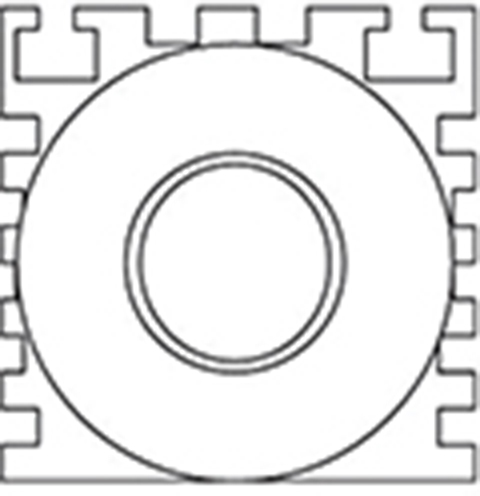
Fig. 10.3. Extruded heat sink — housing of tubular LSM.

Modern motion control systems with tubular LSMs require high-resolution feedback for position control and commutation feedback for controlling the frequency and phase of the three-phase motor signal (Fig. 10.4).

Although tubular PM LSM in comparison with ball or roller screw PM brushless motor linear actuators develop 10 times higher linear speed, provide fully programmable, zero-backlash controllability and emit much lower noise, the maximum force density is only 500 N/kg versus over 1200 N/kg for PM brushless motor linear actuators (Table 10.2).

Images

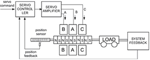
Fig. 10.4. Motion control system with tubular LSM.

Table 10.2. Comparison of tubular LSMs with ball screws

Images

10.3 Linear Positioning Stages

Linear positioning stages have been partially discussed in Chapter 6, Section 6.6. Every motorized positioned stage comprises three essential components: (1) stage, (2) motor, and (3) controller. Positioning stages have travel range from a few micrometers to several meters.

Configurations of positioning stages are shown in Fig. 10.6 [119]. The simplest form of positioning stage is a single-axis stage (Figs 6.17 and 10.6a). It typically consists of a moving table (carriage), base, motor, encoder, limit switches and cable carriers. A compound xy positioning stage (Fig. 10.6b) provides the simplest form of 2 linear DOF of a positioning system where the base of the top axis is bolted to the moving table of the lower axis [119]. A compound xyz stage (Fig. 10.6c) provides the simplest form of 3 linear DOF of a positioning system with the smallest footprint. A split xyz positioning stage (Fig. 10.6d) provides typically higher precision and higher stiffness than a compound configuration of the same number of axes [119].

Images

Fig. 10.5. Two-axis linear positioning stage as an example of replacement ball lead screw mechanisms with tubular LSMs. 1 — x-direction tubular LSM, 2 — y-direction tubular LSM. Courtesy of em ABTech, Swanzey, NH, USA.

Positioning stages with linear motors are far simpler to design and assemble compared to a stage that is based on a rotary motor. The ball screw, coupling, gears, rack-and-pinion, or belts are all eliminated.

The single-axis positioning stage shown in Fig. 10.7 is driven by a three-phase, double-sided PM LBM with ironless core, commutated either sinusoidally or trapezoidally using Hall sensors. The ironless armature assembly has no electromagnetic attractive force to the stationary PM assembly, which reduces the load on and increases the life of the bearing system. The encapsulated armature coil assembly moves, and the multipole PM assembly is stationary. The lightweight coil assembly allows for higher acceleration of light payloads than heavier PM assembly. Linear guidance is achieved by using a single linear rail with one or two linear recirculating ball-bearing guides. The bearing is sealed with wipers to contain the lubrication and to keep out debris.

When neglecting the electrical dynamics of the LSM, the dynamics of a single-axis positioning stage can be described by the following equation:

Images

Fig. 10.6. Configurations of linear positioning stages: (a) single axis, (b) compound xy, (c) compound xyz, (d) split xyz [119].

Images

Fig. 10.7. Single-axis positioning stage with air-cored PM LSM. Photo courtesy of H2W Technologies, Santa Clarita, CA, USA.

m \frac{d^{2} x}{d t^{2}} + D_{υ} \frac{d x}{d t} + k_{s} x + F_{r} + F_{e x t} = k_{F} I_{a} (10.24)

$m \frac{d^{2} x}{d t^{2}} + D_{υ} \frac{d x}{d t} + k_{s} x + F_{r} + F_{e x t} = k_{F} I_{a} (10.24)$

where m is the mass of the moving table, D_v is the damping/friction constant; k_s is the spring constant; F_r is the external disturbance force, e.g., ripple force, F_ext is the external force during manufacturing operation; k_F is the thrust constant (6.6); and I_a is the armature current. Compare eqn (10.24) with eqns (1.25 and (10.9).

A linear precision positioning stage with two LSMs to obtain the x − y motion is shown in Fig. 10.8. Multiaxis linear positioning stages provide a very compact platform for accurate positioning of delicate payloads in high-cycle applications. For example, the extremely smooth running five-axis linear stage shown in Fig. 10.9 enables reduction of the footprint of the machine and, at the same time, maximization of throughput. It is designed for high-speed assembly, test and measurements, grinding, polishing, etc.

Images

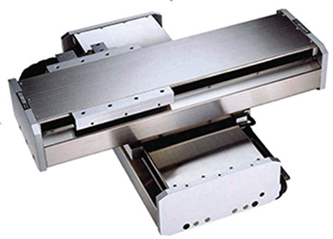
Fig. 10.8. Compound xy positioning stage with two PM LSMs. Photo courtesy of Hiwin Corporation, San Jose, CA, USA.

Images

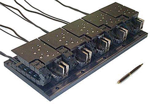
Fig. 10.9. Compact five-axis positioning stage with PM LSMs. Photo courtesy of H2W Technologies, Santa Clarita, CA, USA.

Controllers are units that interface the user with the linear positioning stage. They have computer interfaces and interfaces to the linear motor of the stage. The controller can also be remotely operated. The controller has inputs for encoders of the stage. Most controllers are also programmable by downloading an instruction set onto them. A common programming platform for many controllers is ActiveX¹, which is user friendly.

Typical applications of positioning stages include

precision machinery,
high-precision automation,
pick-and-place,
parts transfer,
semiconductor processing,
optical components manufacturing,
laser machining,
precision metrology,
vision inspection,
clean room.

10.4 Gantry Robots

The term “gantry” defines a system with two motors controlling a single linear axis. Each motor/bearing system is separated a finite distance orthogonal to the direction of the axis. The most common mechanical systems use either linear motors or rotary motors with ballscrews (or belts). A typical gantry configuration is shown in Fig. 10.10.

Gantry robots are also called Cartesian or linear robots. They are usually large systems that perform material handling tasks (palletizing, unitizing, stacking, order picking, and machine loading) and drive-through wash systems for tracks and cars, but they can also be used in manufacturing processes, e.g., welding, removing paint from large aircraft, flat panel manufacture, and coordinate measuring.

A gantry robot consists of a manipulator mounted onto an overhead system that allows movement across a horizontal plane. Each of the motions is arranged to be perpendicular to the other, and are typically labeled x, y, and z. Motions in the x and y directions are located in the horizontal plane, while z is the vertical direction. Specifications in the x and y-axis require an absolute position accuracy of less than ±5.0 mm and repeatability of ±1.0 mm. Gantry robot systems with PM LSMs provide the following advantages:

Large work envelopes (not restricted by arm length)
Less limited by floor space constraints than other robots
Better suited for multiple machines and conveyor lines
Better handling of large or awkward payloads

Images

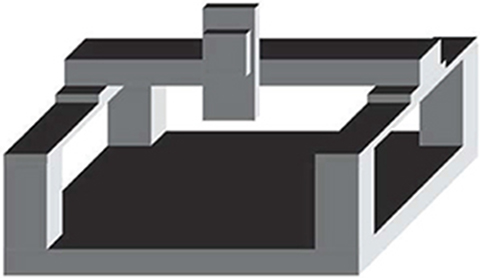
Fig. 10.10. Gantry configuration [119]

Very good positioning accuracy²
Better acceleration
Improved efficiency and versatility
Easy programming with respect to motion, because gantry robots work with xyz coordinate system
Superiority of optimum schedule

Images

Fig. 10.11. Hercules series gantry x-y stages. Photo courtesy Anorad Rockwell Automation, Shirley, NY, USA.

Images

Fig. 10.12. AGS20000 gantry with LSMs. Courtesy of Aerotech, Pittsburgh, PA, USA.

The Hercules family of gantrie (Anorad, Shirley, NY, USA) are designed to address a multitude of performance requirements for inspection, pick-and-place, assembly, or dispensing applications. The Hercules gantry stages (Fig. 10.11) are based on a single platform design, where many linear servo motor selections, linear encoder options, and several travel lengths allow for uniquely supporting a variety of applications with a cost-effective solution. The standard model Hercules gantries feature iron-cored LSMs that are ideally suited to meet the rapid point-to-point motion common in the electronics assembly industry. High force produced by LSMs, combined with a low mass x-axis crossbeam, allows high acceleration to maximize throughput.

Aerotech, Pittsburgh, PA, USA has introduced the AGS20000 gantries with LSMs, which are believed to be the most powerful and accurate Cartesian gantries in the world (Fig. 10.12). Dual PM linear brushless servomotors and dual linear encoders offer [5]:

high velocity up to 3 m/s and high acceleration up to 5g;
lower-axis continuous force 1644 N (air cooling), peak force 3288 N;
upper-axis continuous force 276 N (air cooling), peak force 1106 N;
accuracy ±3.0 mm;
repeatability ±1.0 mm;
resolution 0.02 to 1.0 mm;
optimized mechanical structure for high servo bandwidth.

10.5 Material Handling

10.5.1 Monorail Material Handling System

Fig. 10.13 shows an overhead monorail system for material handling with two HLSMs to obtain a linear motion control in the x and y direction. Such a monorail system can be computer controlled and installed in automated assembly lines or material transfer lines where high precision of positioning or clean atmosphere is required.

Images

Fig. 10.13. Automated monorail system with HLSMs. 1 — overhead monorail, 2 — x-direction forcer of an HLSM, 3 — y-direction forcer of a HLSM.

10.5.2 Semiconductor Wafer Transport

Manual handling and manual semiconductor wafer transport are not an acceptable methods for advanced manufacturing processes. HLSMs simplify the process of semiconductor wafer transport as shown in Fig. 10.14 [40]. The HLSM offers increased throughput and gentle handling of the wafer.

Magnetically levitated wafer transport systems are also used for the semiconductor fabrication process to get rid of the particle and oil contaminations that normally exist in conventional transport systems.

10.5.3 Capsule-Filling Machine

To dispense radioactive fluid into a capsule, an HLSM driven machine can be used. Such a solution has the following advantages [40]:

increased throughput,
no spilling of radioactive fluid,
automation in two axes,
smooth, repeatable motion,
cost-effective solution.

In a capsule-filling machine shown in Fig. 10.15, the forcer of an HLSM moves a tray with empty capsules along a horizontal axis [40]. The filling head driven by a rotary stepping motor and ball lead screw, is raised and lowered in the vertical axis. A linear motor in the vertical axis has also been considered, but with loss of power, the fill head will drop onto the tray [40]. The simple mechanical construction guarantees a long maintenance-free life.

Images

Fig. 10.14. Semiconductor wafer transport. 1 — forcer of HLSM used as a carrier for wafers, 2 — platen, 3 — camera or laser. Courtesy of Parker Hannifin Corporation, Rohnert Park, CA, USA.

Images

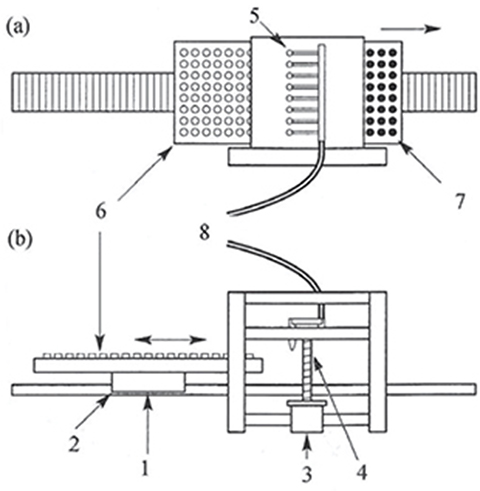
Fig. 10.15. Capsule-filling machine with an HLSM. 1 — forcer, 2 — platen, 3 — rotary microstepping motor, 4 — lead screw, 5 — filling heads, 6 — tray of empty capsules, 7 — full capsules, 8 — hose. Courtesy of Parker Hannifin Corporation, Rohnert Park, CA, USA.

In addition to the foregoing examples of material-handling systems, HLSMs offer solutions to a variety of factory automation systems that include [40]:

printed circuit board assembly,
industrial sewing machines,
light assembly automation,
automatic inspection,
wire harness making,
automotive manufacturing,
gauging,
packaging,
medical applications,
parts transfer,
pick-and-place,
laser cut and trim systems,
flying cutters,
semiconductor technology,
water jet cutting,
print heads,
fiber optics manufacture,
x-y plotters.

Speed, distance, and acceleration are easily programmed in a highly repeatable fashion.

10.6 Machining Processes

The seven basic machining processes are shaping, drilling, turning, milling, sawing, broaching, and abrasive machining. To accomplish the basic machining processes, eight basic types of cutting machine tools have been developed [49]:

shapers and planers,
drill presses,
lathes,
boring machines,
milling machines,
saws,
broaches,
grinders.

For example, constructions of milling machines are shown in Fig. 10.16.

Images

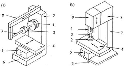
Fig. 10.16. Major components of knee type milling machines with (a) horizontal spindle, (b) vertical spindle. 1 — spindle, 2 — cutter, 3 — arbor, 4 — table, 5 — knee, 6 — base, 7 — column, 8 — overarm, 9 — head.

10.6.1 Machining Centers

Most of machine tools are capable of performing more than one of the basic machining processes. This advantage has led recently to the development of machining centers. A machining center is a specifically designed and numerically controlled (NC) single machine tool with a single workpiece set up to permit several of the basic processes, plus other related processes [49]. Thus, a machining center can perform a variety of processes and change tools automatically while under programmable control. Numerical control is a method of controlling the motion of machine components by means of coded instructions generated by microprocessors or computers.

A part to be machined is fixed to the x-y table of the machining center, which must provide a movement both in the x and y directions (Fig. 10.17). The vertical z movement is provided by the head, e.g., to control the depth of drilled holes. This can also be achieved by moving the cutting tool in the w direction (Fig. 10.17). To obtain the full flexibility of machining, the vertical cutting tool should rotate around its horizontal axis (α direction). Closed-loop position control is used in each of five axes.

In the early 1990s, high-speed modern machining centers have been developed (Makino Milling Company and Comau Company). Specifications of high-speed machining centers are given in Table 10.3 [103]. The maximum speed v_max = 60 m/min is at least twice higher, and the maximum acceleration a_max ≈ 1 g is at least three times higher than those of conventional machining centers. On the other hand, the static servo stiffness of high speed machining centers decreases about 18 times in comparison with conventional machining centers. This is mainly caused by the increase of the pitch τ_l of the screw and decrease of the rotor moment of inertia J_m of the servo motor.

Images

Fig. 10.17. Five-axis vertical spindle machining center. 1 — cutting tool, 2 — table, 3 — machine zero point, 4 — column, 5 — head.

Table 10.3. Specifications of a modern high speed machining center with ball lead screws [103]

Images

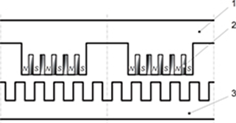
Fig. 10.18. High thrust density PM LBM developed by Shinko Electric Co. Ltd, Japan. 1 — armature core, 2 — PM, 3 — reaction rail.

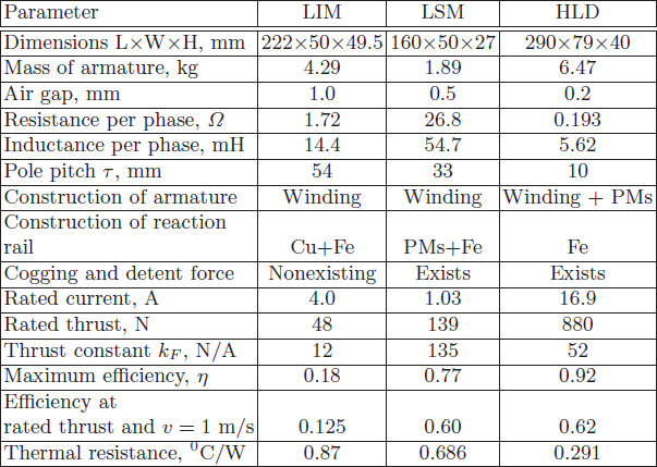
LIMs [63] are not recommended motors for machine tool applications because they emit large amounts of heat and have low efficiency and power factor. PM LSMs or LBMs are much better motors because they are smaller and can provide efficiency over 75%, high power factor, and fast response. According to Shinko Electric Co. Ltd, Takegahana Ise, Japan, the so-called PM high-thrust density linear motor (HDL) has efficiency over 90% at low speed and very high acceleration [105, 155]. An HDL is similar to HLSM, i.e., both have forcer windings and toothed reaction rail; however, the HDL has a different arrangement of PMs (Fig. 10.18). Table 10.4 compares the performance of three different linear motors, i.e., LIM, LSM and HDL for applications to machine tools [103, 155]. The HDL is sometimes called flux reversal PM LSM [38].

The most important variable that describes the behavior of a position control loop for computer numerically controlled (CNC) machine tool driven by a linear motor servo drive is position loop gain K_v [164]. This is the ratio of the command velocity (feed rate) v to the position control deviation (following error, tracking error, lag) Δx, i.e.,

K_{υ} = \frac{υ}{Δ x} 1 / s (10.25)

$K_{υ} = \frac{υ}{Δ x} 1 / s (10.25)$

In general, position loop gain K_v should be high for faster system response and higher accuracy, but the maximum gains allowable are limited due to undesirable oscillatory responses at high gains and low damping factor [164]. Usually, K_v factor is experimentally tuned on the already assembled machine tool. To obtain the required position control loop damping, the position loop gain K_v should be calculated with the following equation [164]

K_{υ} = \frac{1}{4 ζ^{2} (\frac{2 D_{υ}}{w} + \frac{T_{s}}{2})} 1 / s (10.26)

$K_{υ} = \frac{1}{4 ζ^{2} (\frac{2 D_{υ}}{w} + \frac{T_{s}}{2})} 1 / s (10.26)$

where ω is the angular frequency, D_v is the damping constant, ζ is the position control loop damping (0 < ζ < 1), and T_s is the sampling period. In practice, the K_v factor must be decreased up to 40% due to the presence of nonlinearities, i.e.,

Table 10.4. Comparison of linear motors used in servo drives of machine tools

Images

K_{υ} = \frac{0.6}{4 ζ^{2} (\frac{2 D_{υ}}{w} + \frac{T_{s}}{2})} 1 / s (10.27)

$K_{υ} = \frac{0.6}{4 ζ^{2} (\frac{2 D_{υ}}{w} + \frac{T_{s}}{2})} 1 / s (10.27)$

Using eqn (10.27), the position loop gain K_v of a CNC machine tool driven by linear motor servo drive can be estimated without performing any experiments.

First machining centers with linear motor propulsion were built by Ingersoll Milling Machine Company, Rockford, IL, USA and LMT Consortium, Japan [103] in the mid 1990s. In machining centers built by Ingersoll, series LF LSMs manufactured by Anorad [12] have been installed. Table 10.5 shows specifications of the LMT96 machining center manufactured by LMT Consortium [103].

Mazak Corporation, uses linear motors in the F3-660L horizontal machining center shown in Fig. 10.19, which is designed for automotive applications, especially for die-cast aluminum such as transmission casings [53]. This machining center uses LSMs for the x, y and z axes. With a rapid traverse of 120 m/min in the x-axis and 50 m/min on the y and z axes, the table is capable of accelerating at 0.5 g in all axes. Machining centers with LSMs are mainly used for machining processes that require high contouring accuracy, e.g., manufacturing of dies or molds. Contouring permits two or three axes to be controlled simultaneously in two or three dimensions. The price of machining centers with linear motors is almost twice of that with ball lead screws.

Images

Fig. 10.19. Horizontal machining center F3-660L with LSMs for all three axes. Photo courtesy of Mazak Corporation, Florence, KY, USA.

10.6.2 Aircraft Machining

Most wing ribs and floor spars on aircraft are made of stamped sheet metal cut to a contour [131]. Extrusion stock is then riveted to one or both faces to add strength. A small wing rib could be 50 × 250 × 1350 mm in dimension, while floor spars can be up to 0.9 m wide and more than 6 m in length. Since a typical commercial jetliner has around 100 wing ribs and another 100 floor spars, the time in labor, as well as the cumulative weight of the components, tends to add up [131].

Monolithic parts, i.e., structural components hogged out of single billets of metal, usually aluminum, can save time and cost in manufacturing. Making wing ribs, floor spars, fuselage frames, and other parts with pockets and honeycomb structures from single aluminum pieces would use about the same amount of material as sheet metal assembly. The real savings would be in the elimination of hundreds of fasteners, increased production speed, elimination of tooling, and the production of those tools [131]. The main problem has been how to machine these large parts with high speed, efficiency and repeatable accuracy.

The HyperMach program (Boeing, McDonnel Douglas, United Technologies Corporation, and US Air Force as primary partners) has solved this problem with the aid of LSMs. The HyperMach^TMaerospace vertical profiler (Fig. 10.20) with Kollmorgen and Anorad LSMs can make contours at feed rates of over 100 m/min accelerating as fast as 2 g. Machine range is over 0.914 m in the x-axis, 1.5 m in the y-axis, and 0.75 m in the z-axis. This machine platform offers high-efficiency machining for both thin and thick plate processing of a wide variety of large aluminum structural components such as ribs, bulkheads, plate, frames, stringers, and spars to meet the demands of next-generation aircraft parts. The x and y axes are driven by PM LSMs.

Table 10.5. Specifications of machining center LMT96 manufactured by LMT Consortium, Japan

Images

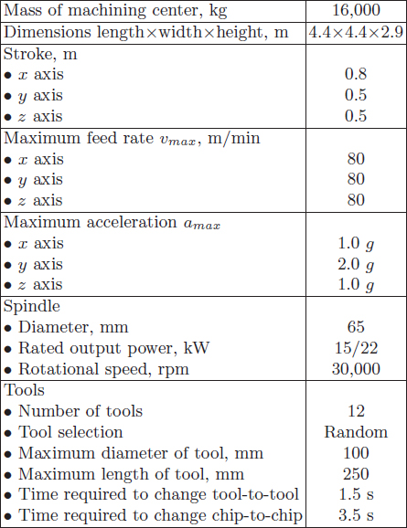
Fig. 10.20. HyperMach^TMvertical profiler with PM LSMs in the x and y axes. Photo courtesy of MAG, Hebron, KY, USA.

Images

Fig. 10.21. IEV flexible vertical grinding center with LSMs. Photo courtesy of Danobat Group, Elgoibar, Spain.

A high precision vertical grinding centre for complete machining of a wide range of aerospace components such as nozzles, ballscrews, landing-gear flaps, etc., is shown in Fig. 10.21. This machining center is designed using LSM technology and precision linear slides.

10.7 Welding and Thermal Cutting

10.7.1 Friction Welding

The heat required for friction welding is produced as a result of mechanical friction between two pieces of metal to be joined [49]. Those two pieces are held together while one rotates and the other is stationary. The rotating part is held in a motor-driven collet, while the stationary part is held against it under controlled pressure produced by a hydraulic or pneumatic actuator (Fig. 10.22a). The frictional heat is a function of the rotational speed and applied pressure (linear force). The rotational speed and force depend on the size of the piece of metal to be welded. For example, for welding a 3 mm mild steel stud, a force about 900 N at 20,000 rpm is required [92].

In manufacturing plants where clean atmosphere is required, hydraulic or pneumatic actuator must be replaced by electric linear actuator (Fig. 10.22b). PM linear actuators [92] or PM LSMs can successfully be used.

10.7.2 Welding Robots

HLSMs provide a simple solution to high-precision motion control of a torch or electrode of welding robots. Fig. 10.23 shows a robot for the resistance spot welding in which the electrode is moved in the x-y plane with the aid of two HLSMs [240]. The robot is microprocessor controlled.

Images

Fig. 10.22. Equipment used for friction welding: (a) with hydraulic or pneumatic actuator, (b) with electric linear actuator. 1 — mechanical actuator, 2 — PM actuator or tubular LSM, 3 — chuck for stationary part, 4 — chuck for rotating part, 5 — spindle, 6 — rotary electric motor.

Images

Fig. 10.23. Linear motor driven welding robot. 1 — arm driven by two HLSMs in x–y plane, 2 — base, 3 — table.

10.7.3 Thermal Cutting

Most of all thermal cutting is done by oxyfuel gas cutting where acetylene is used as a fuel [49]. The tip of the torch contains a circular array of small holes through which the oxygen–acetylene mixture is supplied for the heating flame. In many manufacturing applications, cutting torches cannot be manipulated manually, and electrically driven carriages are used to hold cutting torches. LSMs or LIMs can be used as direct linear drives for torch carriages.

10.8 Surface Treatment and Finishing

10.8.1 Electrocoating

In the electrocoating process, a workpiece is placed in a tank with paint and water solvent. A d.c. voltage is applied between the tank (cathode) and workpiece to be coated (anode). The paint particles are attracted to the workpiece and deposited on it creating a uniform thin coating (0.02 to 0.04 mm) [49]. Then the workpiece is removed from the dip tank, rinsed, and baked at about 195⁰C for 10 to 20 min. This process is especially suitable for complex metal structures such as automobile bodies [49].

Images

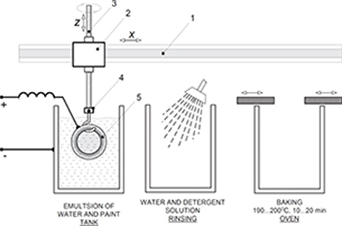
Fig. 10.24. Automated electrocoating line with linear-motor-driven workpieces. 1 — monorail, 2 — LSM or HLSM, 3 — ball lead screw driven by a rotary servo motor (can be replaced by a tubular LSM), 4 — gripper, 5 — workpiece.

Fig. 10.24 shows an automated electrocoating line with linear-motor-driven overhead monorail system for horizontal transfer of bulk workpieces. Depending on the required thrust, mass of the workpiece, and travel distance in the x direction, either LSMs or HLSMs can be used. To raise or lower a heavy workpiece vertically, ball lead screws driven by rotary servo motors are better than linear motors.

10.8.2 Laser Scribing Systems

Aircraft aluminum skin panels are usually scribed manually through templates prior to chemical milling. This costly process can be automated by the use of laser scribers and LSMs [55, 110]. An automatic laser maskant scriber with LSMs was built in 1993 for Boeing, Wichita, KS, USA. [55]. In the chemical milling process, most aircraft component parts are covered with a coating called maskant³. In this etched machining process, the scribed metal surface is coated with polymer material. The laser process is kept smoke free, and the scribed line is kept clean through the use of the smoke extraction hood installed on the optical laser wrist. The polymer is scribed to a desired pattern and then removed from the surface. The metal is then placed in an acid solution that etches out the exposed surfaces.

Two parallel LSMs, (series LF, Anorad[12]) produce the peak thrust up to 9 kN at speed up to 5 m/s [110]. LSMs rapidly and precisely position a huge gantry with the CO₂ laser maskant scribing system. Two laser systems have been used: one for scribing and another for position feedback. The use of a laser interferometer for positioning feedback with LSM drive mechanisms results in high accuracy and repeatability. Large over 30 m long 5-axis gantry for laser maskant scriber driven by Anorad’s LSMs is shown in Fig. 10.25.

Images

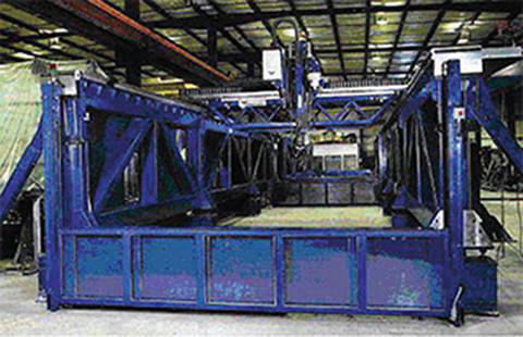
Fig. 10.25. Large 5-axis gantry for laser maskant scriber driven by Anorad’s LSMs. Photo courtesy of G. Hagiz [76].

The advantages of the new LSM driven laser maskant scriber include mass, scrap and inventory reduction, noncontact design, no lubrication and adjustments, elimination of the stress channel, and minimizing back bending and repetitive motions. According to Boeing, this is the largest automatic laser scriber in the world (33 m long, 3 m wide, and 5.1 m tall) that can hold two Boeing 747 wings simultaneously, scribing one while positioning the other and scribe up to 2.54 m/s or complete up to four skin panels in 1 h [110].

Images

Fig. 10.26. UVS 5-axis machining center with Siemens SIMODRIVE LSM 840D CNC for aircraft industry: (a) overhead gantry (b) Airbus A320 external skin around front landing box to be laser processed. Photo courtesy of Le Creneau Industriel, Annecy le Vieux, France.

Le Creneau Industriel, Annecy le Vieux, France, is a manufacturer of 5 axis machining centers (Fig. 10.26) for routing and drilling aluminum and large-dimension composite components for the aircraft industry. The UGV 5 axis machine with overhead moving gantry, Coherent 100 W CO₂ laser, and optical laser wrist, have been designed for aircraft manufacturers for laser-scribing maskant prior to chemical machining [75].

The optical laser wrist is designed with a large 9 m×4.5 m ×1.5 m work envelope moving gantry. It incorporates a Siemens Simodrive 840D CNC with 1FN LSMs to provide high accuracy with speeds up to 60 m/min [75]. The curved component to be laser processed is placed on a 99-peg support fixture where each peg has its own independent numerical axis to form the precise 3D shape required. The optical laser wrist incorporates a measurement probe to confirm the actual shape of the component prior to being laser processed. The result is compared to the theoretical shape within the system’s software for quality control. The complex pattern is scribed up to 30 m/min with an accuracy of ±0.025 mm.

10.8.3 Application of Flux-Switching PM Linear Motors

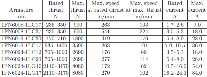
Large gantry systems and machining centers require powerful linear motors, preferably with PM-free reaction rail. Siemens 1FN6 PM LSMs with a magnet-free reaction rail belong to the group of the so called flux-switching PM machines [90, 176]. The armature system is air cooled, degree of protection IP23, class of insulation F, line voltage from 400 to 480 V, rated thrust from 235 to 2110 N, maximum velocity at rated thrust from 170 to 540 m/min (Table 10.6), overload capacity 3.8 of rated thrust, modular type construction [198]. These LSMs operate with Siemens Sinamics or Simodrive solid-state converters and external encoders. According to Siemens [198], these new LSMs (Fig. 10.27) produce thrust forces and velocities equivalent to competitive classical models for light-duty machine tool, machine accessory, and material handling applications.

Table 10.6. Specifications of 1FN6 PM LSMs manufactured by Siemens, Erlangen, Germany [198]

Images

The magnet-free reaction rail is easy to install and does not require the safety considerations of standard PM reaction rails. Without PMs, there is no problem with ferrous chips and other debris being attracted to these sections. Maintenance becomes a simple matter of installing a wiper or brush on the moving part of the slide.

The 1FN6 flux-switching LSMs comprises an armature section that is equipped with coils and PMs as well as a nonmagnetic, toothed reaction rail section (Fig. 10.28). The key design innovation is an LSM in which PMs are integrated directly into the lamination of the armature core along with the individual windings for each phase. Both magnitudes and polarities of the linkage flux in the armature winding vary periodically along with the reaction rail movement. The magnetic flux between the armature core and steel reaction rail is controlled by switching the three-phase armature currents according to a designated algorithm [172]. The passive reaction rail consists of milled steel with poles (teeth) and is much simpler to manufacture.

The relationships between the pole pitches and number of poles of the armature and reaction rail are

τ_{2} = \frac{τ_{1}}{1 \pm \frac{k}{m_{1}}} (10.28)

$τ_{2} = \frac{τ_{1}}{1 \pm \frac{k}{m_{1}}} (10.28)$

Images

Fig. 10.27. Novel 1FN6 flux-switching LSM with PM-free reaction rail. Photo courtesy of Siemens AG, Erlangen, Germany.

Images

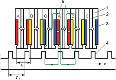
Fig. 10.28. Construction of flux-switching LSM with PM-free reaction rail. 1 — laminated armature core, 2 — PM, 3 — armature coil (phase C), 4 — toothed passive steel reaction rail, 5 — linkage magnetic flux (phase A is on).

P_{2} = P_{1} \frac{τ_{1}}{τ_{2}} (10.29)

$P_{2} = P_{1} \frac{τ_{1}}{τ_{2}} (10.29)$

where τ₁, τ₂ are pole pitches of the armature and reaction rail, respectively, P₁ and P₂ are the numbers of the armature and reaction rail poles, respectively, and k = 1, 2, 3, … is integer. For example, if τ₁ = 42 mm, m₁ = 3 and k = 1, the reaction rail pole pitch τ₂ = 42/[1±(1/6)] = 36 mm or 50.4 mm. Assuming P₁ = 12, the possible number of reaction rail poles is P₂ = 12 × (42/36) = 14 or P₂ = 12 × (42/50.4) = 10.

As far as the authors are aware, the first paper on flux-switching PM brushless rotary machines was published in 1955 [176]. There are numerous papers on the analysis of this type of machines, e.g., [21, 37, 90, 94, 251]. However, it is impossible to find a convincing analysis published so far on how flux-switching PM brushless motors compare to standard PM brushless motors in terms of thrust density, efficiency, and power factor. Some constructions of flux-switching PM LSMs have been patented [P212, P213, P215].

10.9 2D Orientation of Plastic Films

High-quality plastic films can be obtained as a result of simultaneous orientation technology in which the film is stretched in two directions [32]. Simultaneous orientation is a process where the distances between clips, i.e., gripping points of the film, are continuously increased as a result of moving clips apart lengthwise and across.

Images

Fig. 10.29. Application of LSMs to simultaneous film orientation technology. 1 — LSM, 2 — driven clips, 3 — idle clips, 4 — cast film, 5 — oriented film. Courtesy of Brueckner Maschinenbau GmbH, Siegsdorf, Germany.

LSMs can be used to move clips forward with adjustable speeds [32]. Driven carriages (clips) with built-in PMs are arranged in a closed circuit to form a roller rail (Fig. 10.29). Armature systems of LSMs are stationary. Additional gripping points for the film are provided by idle carriages that move between driven carriages. Each carriage can move freely along the rail without any mechanical limitations. As many as 900 LSMs with rated thrust of 900 N each can be employed, and linear velocities up to 7.5 m/s (450 m/min) can be achieved [32]. The working width of foil is 7.5 m, and the length of the track is 2×126 m. High speeds and flexibility of speed sequences of individual carriages allow for high productivity and adjustable product features.

The electromagnetic thrust of each LSM is proportional to the load (power) angle δ, i.e., F_dx ≈ (m₁/v_s)(V₁E_f/X_sd) sin δ. Variation of external forces causes variation of the angle δ and, as a consequence, oscillations are generated. To damp oscillations effectively, an active damping control system is implemented in addition to the damper. An observer estimates the load angle δ from the known currents and sends a feedback to the controller [32].

10.10 Testing

10.10.1 Surface Roughness Measurement

Roughness is measured by the heights of irregularities with respect to an average (center) line [49]. Most instruments for measuring surface roughness use a diamond stylus that is moved at a constant speed. The vertical movement of the stylus is usually detected with the aid of a linear variable differential transformer (LVDT), and as an electrical signal can be processed electronically and stored on the computer disk or recorded on a strip chart. The unit containing the stylus can be driven by two HLSMs in the x-y plane (Fig. 10.30). After making a series of parallel offset traces on the tested surface, a

Images

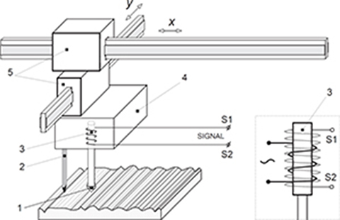
Fig. 10.30. Stylus profile device for measuring surface roughness and profile. 1 — diamond stylus, 2 — rider, 3 — LVDT, 4 — head, 5 — HLSM.

10.10.2 Generator of Vibration

Analysis and simulation of dynamic behavior of buildings and large-scale constructions requires long-stroke and high-speed generators of vibration. Typical parameters of such a device are: 7.7 kN maximum thrust, 6.5 kN rated thrust, 2 m/s maximum speed, 0.5 m effective stroke, and 2000 kg maximum load mass [105]. Oil hydraulic devices are large, need complex maintenance, and have low efficiency and nonlinear characteristics. Linear electric actuators or motors are smaller, provide high speed and acceleration, and do not need maintenance. Shinko Electric Co. Ltd has built a prototype generator of vibration with HDL [105]. A good response, i.e., thrust versus sinusoidal current signal, has been obtained in the vibration domain less than 5 Hz.

10.11 Industrial Laser Applications

Laser systems driven by LSM x-y positioning stages have been sucessfully applied to diamond processing, including sawing, cutting, kerfing, and shaping [55]. Advantages of applications of LSMs versus ball lead screws include better-quality finished surface, insensitivity of LSMs to diamond dust, and positioning accuracy of 0.2 μm over travel distances 300 by 100 mm. A multitask diamond processing laser system has been built by Or-Ziv, Rehovot, Israel [55].

A linear motor gantry for industrial laser-cutting systems has been built e.g., by CBLT, Starnberg, Germany [55]. High-beam-quality CO₂ laser together with LBM positioning stages provide smoother cuts, more vertical surfaces and cleaner edges.

Large laser scribing-systems with LSMs have been described in Section 10.8.2.

Examples

Example 10.1

A linear ball screw system driven by a rotary PM brushless motor has the following parameters: maximum rotational speed of the motor n = 2400 rpm, maximum stator current I_amax = 8.0 A, torque constant k_T = 2.255 Nm/A, mass of the rotor m_r = 5.2 kg, diameter of the rotor D_r = 48 mm, diameter of ball screw d_b = 32 mm, mass of ball screw m_b = 4.4 kg, pitch of screw τ_l = 11 mm, number of threads k = 1 (single start screw), number of teeth on the motor wheel N₁ = 54, number of teeth on the ball screw wheel N₂ = 18, and mass of the table m_t = 4.6 kg. Find the maximum linear acceleration and dynamic stiffness of the ball screw drive.

Solution

The maximum rotational speed of the ball screw

n_{b} = \frac{N_{2}}{N_{1}} n = \frac{54}{18} \times 2400 = 800 rpm = 13.33 rev / s

$n_{b} = \frac{N_{2}}{N_{1}} n = \frac{54}{18} \times 2400 = 800 rpm = 13.33 rev / s$

For k = 1 (single start screw) according to eqn (10.3), the lead is equal to the screw pitch, i.e., l = 1 × 11 = 11 mm, and maximum linear speed according to eqn (10.8) is v_max = 13.33 × 0.011 = 0.147 m/s = 8.8 m/min. The various moments of inertia are as follows

Moment of inertia of the motor cylindrical rotor

$J_{m} = \frac{1}{2} m_{r} \frac{D_{r}^{2}}{4} = \frac{1}{2} 5.2 \frac{{0.048}^{2}}{4} = 1.498 \times 10^{- 3} {kgm}^{2}$ $J_{m} = \frac{1}{2} m_{r} \frac{D_{r}^{2}}{4} = \frac{1}{2} 5.2 \frac{{0.048}^{2}}{4} = 1.498 \times 10^{- 3} {kgm}^{2}$
Moment of inertia of the cylindrical ball screw

$J_{b s} = \frac{1}{2} m_{b} \frac{d_{b}^{2}}{4} = \frac{1}{2} 4.4 \frac{{0.032}^{2}}{4} = 0.563 \times 10^{- 3} {kgm}^{2}$ $J_{b s} = \frac{1}{2} m_{b} \frac{d_{b}^{2}}{4} = \frac{1}{2} 4.4 \frac{{0.032}^{2}}{4} = 0.563 \times 10^{- 3} {kgm}^{2}$
Equivalent moment of inertia of the motor–ball screw system according to eqn (10.19)

$J_{e} = 0.563 \times 10^{- 3} + {(\frac{54}{18})}^{2} \times 1.498 \times 10^{- 3} = 0.014 {kgm}^{2}$ $J_{e} = 0.563 \times 10^{- 3} + {(\frac{54}{18})}^{2} \times 1.498 \times 10^{- 3} = 0.014 {kgm}^{2}$

Maximum torque produced by the rotary PM brushless motor

T_{\max} = k_{T} I_{a m a x} = 2.255 \times 8.0 = 18.04 Nm

$T_{\max} = k_{T} I_{a m a x} = 2.255 \times 8.0 = 18.04 Nm$

Maximum output power of the motor

P_{o u t} = 2 π \frac{2400}{60} \times 18.04 = 4534 W

$P_{o u t} = 2 π \frac{2400}{60} \times 18.04 = 4534 W$

Linear acceleration according to eqn (10.22)

a_{m a x} \approx \frac{18.04 \times 0.011}{2 π [0.014 + 4.6 {(\frac{0.011}{2 π})}^{2}]} = 2.247 m / s^{2}

$a_{m a x} \approx \frac{18.04 \times 0.011}{2 π [0.014 + 4.6 {(\frac{0.011}{2 π})}^{2}]} = 2.247 m / s^{2}$

Angular frequency of ball screw

ω = 2 π \frac{800}{60} = 83.78 rad / s

$ω = 2 π \frac{800}{60} = 83.78 rad / s$

Dynamic stiffness according to eqn (10.21)

K_{d} \approx [4.6 + {(\frac{2 π}{0.011})}^{2} \times 0.014] \times {83.78}^{2} = 32.19 \times 10^{6} N / m

$K_{d} \approx [4.6 + {(\frac{2 π}{0.011})}^{2} \times 0.014] \times {83.78}^{2} = 32.19 \times 10^{6} N / m$

Example 10.2

A gantry is driven by a flat PM LSM. The steady-state speed is vconst = 4.0 m/s, overall time of operation t = 1.2 s, acceleration time t₁ = 0.2 and deceleration time t₃ = 0.25 s. For the speed profile given in Fig. 1.22a, find the maximum acceleration, maximum deceleration, and estimate how the thrust will change if (a) the overall time is extended to 1.2t, and (b) the acceleration time t₁ is reduced twice. In both cases, assume that all other parameters are the same.

Solution

Total distance

\begin{matrix} s = \frac{1}{2} υ t_{1} + υ t_{2} + \frac{1}{2} υ t_{3} = \frac{1}{2} υ (t_{1} + t_{3}) + υ (t - t_{1} - t_{3}) \\ = υ t - \frac{1}{2} υ (t_{1} + t_{3}) = 4.0 \times 1.2 - \frac{1}{2} 4.0 \times (0.2 + 0.25) = 3.9 m \end{matrix}

$\begin{matrix} s = \frac{1}{2} υ t_{1} + υ t_{2} + \frac{1}{2} υ t_{3} = \frac{1}{2} υ (t_{1} + t_{3}) + υ (t - t_{1} - t_{3}) \\ = υ t - \frac{1}{2} υ (t_{1} + t_{3}) = 4.0 \times 1.2 - \frac{1}{2} 4.0 \times (0.2 + 0.25) = 3.9 m \end{matrix}$

Maximum acceleration

a_{m a x} = \frac{υ}{t_{1}} = \frac{s}{t_{1} (t - 0.5 t_{1} - 0.5 t_{3})} = \frac{3.9}{0.2 (1.2 - 0.5 \times 0.2 - 0.5 \times 0.25)} = 20 m / s^{2}

$a_{m a x} = \frac{υ}{t_{1}} = \frac{s}{t_{1} (t - 0.5 t_{1} - 0.5 t_{3})} = \frac{3.9}{0.2 (1.2 - 0.5 \times 0.2 - 0.5 \times 0.25)} = 20 m / s^{2}$

Maximum deceleration

d_{m a x} = \frac{υ}{t_{3}} = \frac{s}{t_{3} (t - 0.5 t_{1} - 0.5 t_{3})} = \frac{3.9}{0.25 (1.2 - 0.5 \times 0.2 - 0.5 \times 0.25)} = 16 m / s^{2}

$d_{m a x} = \frac{υ}{t_{3}} = \frac{s}{t_{3} (t - 0.5 t_{1} - 0.5 t_{3})} = \frac{3.9}{0.25 (1.2 - 0.5 \times 0.2 - 0.5 \times 0.25)} = 16 m / s^{2}$

How will the thrust change, if the overall time is extended to 1.2t at the same speed, acceleration, and deceleration time? Since the thrust is proportional to the acceleration, the thrust will decrease by the factor

\frac{t - 0.5 t_{1} - 0.5 t_{3}}{1.2 t - 0.5 t_{1} - 0.5 t_{3}} = \frac{1.2 - 0.5 \times 0.2 - 0.5 \times 0.25}{1.2 \times 1.2 - 0.5 \times 0.2 - 0.5 \times 0.25} = 0.802

$\frac{t - 0.5 t_{1} - 0.5 t_{3}}{1.2 t - 0.5 t_{1} - 0.5 t_{3}} = \frac{1.2 - 0.5 \times 0.2 - 0.5 \times 0.25}{1.2 \times 1.2 - 0.5 \times 0.2 - 0.5 \times 0.25} = 0.802$

The required thrust will decrease. If the existing LSM is rated, say, at 2000 N, for longer overall time, a smaller LSM rated at 0.8×2000 = 1600 N is needed.

How will the thrust change if the acceleration time is reduced to 0.5t₁ at the same speed, acceleration, and deceleration time? Again, the thrust is proportional to the acceleration, i.e.,

\frac{t_{1}}{0.5 t_{1}} = 2

$\frac{t_{1}}{0.5 t_{1}} = 2$

If the existing LSM is rated at 2000 N, for faster acceleration, an LSM with doubled thrust is necessary.

Example 10.3

The model of an LSM-driven positioning stage with mass m_p, spring constant k_sp, and viscous friction coefficient D_vp is shown in Fig. 10.31. The mass m_p includes the mass of LSM and positioning stage. The mass of external structure (load) is m, spring constant k_s, and coefficient of viscous friction D_v. The thrust developed by a linear motor is F_dx(t) and the external (load) force is F_ext(t). Find the equations of motion using:

Free-body diagram;
Euler–Lagrange equation (1.43).

Solution

(a) Free-body diagram

This is a two-DOF system subjected to external forces (Fig. 10.31a). A free-body diagram is shown in Fig. 10.31b. According to eqn (1.28), the mechanical balance equations are

\begin{matrix} F_{d x} (t) - D_{υ p} {\dot{x}}_{1} - k_{s p} x_{1} + D_{υ} ({\dot{x}}_{2} - {\dot{x}}_{1}) + k_{s} (x_{2} - x_{1}) = m_{p} {\ddot{x}}_{1} \\ F_{e x t} (t) - D_{υ} ({\dot{x}}_{2} - {\dot{x}}_{1}) - k_{s} (x_{2} - x_{1}) = m {\ddot{x}}_{2} \end{matrix}

$\begin{matrix} F_{d x} (t) - D_{υ p} {\dot{x}}_{1} - k_{s p} x_{1} + D_{υ} ({\dot{x}}_{2} - {\dot{x}}_{1}) + k_{s} (x_{2} - x_{1}) = m_{p} {\ddot{x}}_{1} \\ F_{e x t} (t) - D_{υ} ({\dot{x}}_{2} - {\dot{x}}_{1}) - k_{s} (x_{2} - x_{1}) = m {\ddot{x}}_{2} \end{matrix}$

m_{p} {\ddot{x}}_{1} + (D_{υ p} + D_{υ}) {\dot{x}}_{1} - D_{υ} {\dot{x}}_{2} + (k_{s p} + k_{s}) x_{1} - k_{s} x_{2} = F_{d x} (t) (10.30)

$m_{p} {\ddot{x}}_{1} + (D_{υ p} + D_{υ}) {\dot{x}}_{1} - D_{υ} {\dot{x}}_{2} + (k_{s p} + k_{s}) x_{1} - k_{s} x_{2} = F_{d x} (t) (10.30)$

m {\ddot{x}}_{2} + D_{υ} {\dot{x}}_{2} - D_{υ} {\dot{x}}_{1} + k_{s} x_{2} - k_{s} x_{1} = F_{e x t} (t) (10.31)

$m {\ddot{x}}_{2} + D_{υ} {\dot{x}}_{2} - D_{υ} {\dot{x}}_{1} + k_{s} x_{2} - k_{s} x_{1} = F_{e x t} (t) (10.31)$

It is more convenient to write eqns (10.30) and (10.31) in matrix–vector form, i.e.,

\begin{matrix} [\begin{matrix} m_{p} & 0 \\ 0 & m \end{matrix}] [\begin{matrix} {\ddot{x}}_{1} \\ {\ddot{x}}_{2} \end{matrix}] + [\begin{matrix} D_{υ p} + D_{υ} & - D_{υ} \\ D_{υ} & D_{υ} \end{matrix}] [\begin{matrix} {\dot{x}}_{1} \\ {\dot{x}}_{2} \end{matrix}] \\ + [\begin{matrix} k_{s p} + k_{s} & - k_{s} \\ - k_{s} & k_{s} \end{matrix}] [\begin{matrix} x_{1} \\ x_{2} \end{matrix}] = [\begin{matrix} F_{d x} (t) \\ F_{e x t} (t) \end{matrix}] \end{matrix} (10.32)

$\begin{matrix} [\begin{matrix} m_{p} & 0 \\ 0 & m \end{matrix}] [\begin{matrix} {\ddot{x}}_{1} \\ {\ddot{x}}_{2} \end{matrix}] + [\begin{matrix} D_{υ p} + D_{υ} & - D_{υ} \\ D_{υ} & D_{υ} \end{matrix}] [\begin{matrix} {\dot{x}}_{1} \\ {\dot{x}}_{2} \end{matrix}] \\ + [\begin{matrix} k_{s p} + k_{s} & - k_{s} \\ - k_{s} & k_{s} \end{matrix}] [\begin{matrix} x_{1} \\ x_{2} \end{matrix}] = [\begin{matrix} F_{d x} (t) \\ F_{e x t} (t) \end{matrix}] \end{matrix} (10.32)$

The short form of the matrix–vector notation

[m] [\ddot{x}] + [D_{υ}] [\dot{x}] + [k_{s}] [x] = [F (t)] (10.33)

$[m] [\ddot{x}] + [D_{υ}] [\dot{x}] + [k_{s}] [x] = [F (t)] (10.33)$

The mass matrix in eqn (10.32) is diagonal, so the system is uncoupled inertially. The damping and stiffness matrices in eqn (10.32) are coupled.

Images

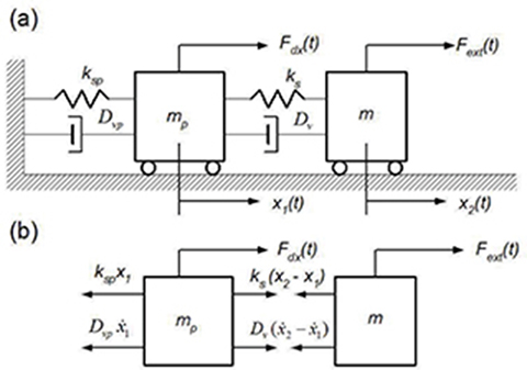
Fig. 10.31. Mathematical model of a single-axis positioning stage driven by a linear motor: (a) two-DOF system subjected to forces F_dx(t) and F_x(t); (b) free-body diagrams.

(b) Euler–Lagrange equation

Kinetic energy, potential energy, and Rayleigh dissipation function (1.44) for ξ = x are, respectively,

E_{k} = \frac{1}{2} m_{p} {\dot{x}}_{1}^{2} + \frac{1}{2} m {\dot{x}}_{2}^{2} (10.34)

$E_{k} = \frac{1}{2} m_{p} {\dot{x}}_{1}^{2} + \frac{1}{2} m {\dot{x}}_{2}^{2} (10.34)$

E_{p} = \frac{1}{2} k_{s p} x_{1}^{2} + \frac{1}{2} k_{s} {(x_{2} - x_{1})}^{2} = \frac{1}{2} k_{s p} x_{1}^{2} + \frac{1}{2} k_{s} x_{2}^{2} - k_{s} x_{1} x_{2} + \frac{1}{2} k_{s} x_{1}^{2} (10.35)

$E_{p} = \frac{1}{2} k_{s p} x_{1}^{2} + \frac{1}{2} k_{s} {(x_{2} - x_{1})}^{2} = \frac{1}{2} k_{s p} x_{1}^{2} + \frac{1}{2} k_{s} x_{2}^{2} - k_{s} x_{1} x_{2} + \frac{1}{2} k_{s} x_{1}^{2} (10.35)$

R a = \frac{1}{2} D_{υ p} {\dot{x}}_{1}^{2} + \frac{1}{2} D_{υ} {({\dot{x}}_{2} - {\dot{x}}_{1})}^{2} = \frac{1}{2} D_{υ p} {\dot{x}}_{1}^{2} + \frac{1}{2} D_{υ} {\dot{x}}_{2}^{2} - D_{υ} {\dot{x}}_{1} {\dot{x}}_{2} + \frac{1}{2} D_{υ} {\dot{x}}_{1}^{2} (10.36)

$R a = \frac{1}{2} D_{υ p} {\dot{x}}_{1}^{2} + \frac{1}{2} D_{υ} {({\dot{x}}_{2} - {\dot{x}}_{1})}^{2} = \frac{1}{2} D_{υ p} {\dot{x}}_{1}^{2} + \frac{1}{2} D_{υ} {\dot{x}}_{2}^{2} - D_{υ} {\dot{x}}_{1} {\dot{x}}_{2} + \frac{1}{2} D_{υ} {\dot{x}}_{1}^{2} (10.36)$

Derivatives with respect to ẋ₁, x₁, and t for the positiong stage with mass m_p taken according to the definion of Lagrangian (1.33) and Euler–Lagrange equation (1.43), are

\begin{matrix} \begin{matrix} \frac{\partial L}{\partial {\dot{x}}_{1}} = \frac{\partial (E_{k} - E_{p})}{\partial {\dot{x}}_{1}} = m_{p} {\dot{x}}_{1}; & \frac{d}{d t} \frac{\partial L}{\partial {\dot{x}}_{1}} = m_{p} {\ddot{x}}_{1} \end{matrix} \\ \frac{\partial L}{\partial x_{1}} = \frac{\partial (E_{k} - E_{p})}{\partial x_{1}} = - k_{s p} x_{1} + k_{s} x_{2} - k_{s} x_{1} \end{matrix}

$\begin{matrix} \begin{matrix} \frac{\partial L}{\partial {\dot{x}}_{1}} = \frac{\partial (E_{k} - E_{p})}{\partial {\dot{x}}_{1}} = m_{p} {\dot{x}}_{1}; & \frac{d}{d t} \frac{\partial L}{\partial {\dot{x}}_{1}} = m_{p} {\ddot{x}}_{1} \end{matrix} \\ \frac{\partial L}{\partial x_{1}} = \frac{\partial (E_{k} - E_{p})}{\partial x_{1}} = - k_{s p} x_{1} + k_{s} x_{2} - k_{s} x_{1} \end{matrix}$

\frac{\partial R a}{\partial {\dot{x}}_{1}} = D_{υ p} {\dot{x}}_{1} - D_{υ} {\ddot{x}}_{2} + D_{υ} {\dot{x}}_{1}

$\frac{\partial R a}{\partial {\dot{x}}_{1}} = D_{υ p} {\dot{x}}_{1} - D_{υ} {\ddot{x}}_{2} + D_{υ} {\dot{x}}_{1}$

Similar derivatives can be taken with respect to ẋ₂, x₂, and t for the linear motor with mass m. Upon substituting derivates, Euler–Lagrange equation (1.43) gives similar equations of motions as eqns (10.30) and (10.31).

^¹ActiveX is a loosely defined set of technologies developed by Microsoft for sharing information among different applications.

^²Position accuracy is the ability of the robot to place a part correctly.

^³Maskant is a material that protects a metal surface during the etching process.

..................Content has been hidden....................

You can't read the all page of ebook, please click here login for view all page.

Table of Contents for
10 Industrial Automation Systems

10

Industrial Automation Systems

10.1 Automation of Manufacturing Processes

10.2 Ball Lead Screws

10.2.1 Basic Parameters

10.2.2 Ball Lead Screw Drives

10.2.3 Replacement of Ball Screws with LSMs

10.3 Linear Positioning Stages

10.4 Gantry Robots

10.5 Material Handling

10.5.1 Monorail Material Handling System

10.5.2 Semiconductor Wafer Transport

10.5.3 Capsule-Filling Machine

10.6 Machining Processes

10.6.1 Machining Centers

10.6.2 Aircraft Machining

10.7 Welding and Thermal Cutting

10.7.1 Friction Welding

10.7.2 Welding Robots

10.7.3 Thermal Cutting

10.8 Surface Treatment and Finishing

10.8.1 Electrocoating

10.8.2 Laser Scribing Systems

10.8.3 Application of Flux-Switching PM Linear Motors

10.9 2D Orientation of Plastic Films

10.10 Testing

10.10.1 Surface Roughness Measurement

10.10.2 Generator of Vibration

10.11 Industrial Laser Applications

Examples

Table of Contents for 10 Industrial Automation Systems

Create new playlist

Sign In

Sign Up

Table of Contents for
10 Industrial Automation Systems