
5
Hybrid and Special Linear Permanent Magnet Motors
5.1 Permanent Magnet Hybrid Motors
5.1.1 Finite Element Approach
The magnetic circuits of stepping motors are frequently highly saturated. Therefore, it is often difficult to calculate and analyze motor performance with consistent accuracy by using the classical circuital or field approach. Using the finite element method (FEM) or other numerical methods, more accurate results can be obtained. Since the hybrid linear stepping motor (HLSM) consists of two independent stacks, it is acceptable to model each stack separately. There is one potential difficulty in the modeling of the HLSM. This arises as a result of the tiny air gap, below 0.05 mm. For better accuracy of the calculation, the air gap requires three or four layers of elements, which in turn leads to high aspect ratios.
The fundamentals of the FEM can be found in Chapter 4 and many monographs, e.g., [41, 70, 189, 236]. In the FEM, both the virtual work method — eqn (1.13) and Maxwell stress tensor — eqn (4.13), can be used for the thrust (tangential force) Fdx and normal force Fdz calculations. Forces calculated on the basis of the Maxwell stress tensor (4.13) are
where Li is the width of the HLSM stack, Bx is the tangential component of the magnetic flux density, Bz is the normal component of the magnetic flux density, and l is the integration path. In the method of virtual work, x is the horizontal displacement between forcer and platen, z is the vertical displacement, and W is the energy stored in the magnetic field — eqn (1.13).
The classical virtual work method needs two solutions, and the choice of suitable displacement has direct influence on the calculation accuracy. The following one solution approach based on Coulomb and Meunier’s method [46] has been used and implemented here for calculating the tangential force
where B is the matrix of magnetic flux density in the air gap region, BT is the transpose matrix of B, |Q| is the determinant of the Jacobian matrix, and Ve is the volume of an element e. For linear triangular elements, the above equation can further be simplified to the following form:
Similarly, the dual formulation for calculating the normal force is obtained as
In eqns (5.3) and (5.4), x and z are rectangular coordinates of the 2D model, e and i are the numbers of virtually distorted elements and virtually moved nodes within an element, respectively, and subscripts 1, 2 and 3, correspond to the nodes of a triangular element. The parameters Δ1 and Δ2 are defined as
where A1 to A3 are magnitudes of the magnetic vector potential corresponding to each node of a triangular element. The Jacobian matrix becomes
5.1.2 Reluctance Network Approach
In recent years, much research has been done on the modeling of electromechanical energy conversion devices by using the reluctance network approach (RNA). Part of this research relates to stepping motors [107, 108, 138, 174]. The RNA is simpler than the FEM and does not require a long computation time [225].
As shown in Fig. 5.1, the fluxes of individual poles are dependent on the PM MMF, winding current, and reluctances. The PM flux ΦM circulates in the main loop while the winding excitation fluxes ΦA and ΦB create local flux loops. Apart from these fluxes, a leakage flux exists that takes a path entirely or partially through the air or nonferromagnetic parts of the forcer. The amount of such a flux is small as compared with the main flux and can, therefore, be neglected. The equivalent magnetic circuit is shown in Fig. 5.2a.
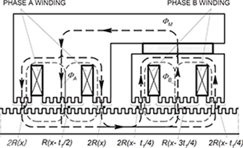
Fig. 5.1. The outline of the magnetic circuit of an HLSM.
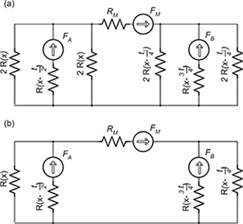
Fig. 5.2. Equivalent magnetic circuit of a two-phase HLSM: (a) magnetic circuit corresponding to Fig. 5.1; (b) simplified magnetic circuit with equal numbers of teeth per pole.
After further simplification, the magnetic circuit can be brought to that in Fig. 5.2b, in which the FM, FA, and FB are MMFs of the PM and phase windings A and B, respectively; ℜ(x), , and are the reluctances of a single pole that vary with tooth alignments, and t1 is the tooth pitch.
Since a highly permeable steel is used in both the forcer and platen, only the air gap and PM reluctances are taken into account. For a pole consisting of n teeth, the reluctance of the air gap corresponding to one pole is
where ℜt = 1/Gt stands for the reluctance of the air gap corresponding to one tooth pitch t1. The calculated reluctance of the air gap over one tooth pitch is shown in Fig. 5.3. For an unsaturated magnetic circuit (μ → ∞) as in Figs 5.4c and 5.4d, all flux lines are perpendicular to ferromagnetic surfaces. As the teeth begin to saturate, the flux paths in the air change their shapes.
The toothed surface of the forcer and platen involves the permeance variation with respect to the linear displacement x according to a periodical function. The following cosinusoidal approximation can be used [36]:
where the maximum permeance Gmax and minimum permeance Gmin can be expressed as
and c and b are tooth and slot width, respectively. The approximation can further help in finding the derivative of reluctance with regard to the displacement, i.e.,
The calculated permeance of the air gap over one tooth pitch t1 and its cosi-nusoidal approximation [36] are plotted in Fig. 5.5.
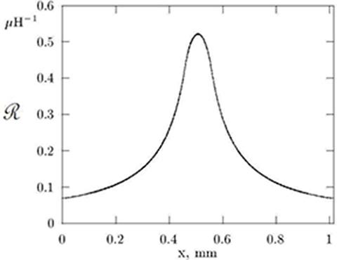
Fig. 5.3. Air gap reluctance distribution over one tooth pitch.
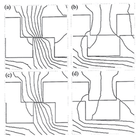
Fig. 5.4. Flux patterns: (a) partially aligned teeth (saturated magnetic circuit), (b) complete misalignment of teeth (saturated magnetic circuit), (c) partially aligned teeth (unsaturated magnetic circuit), (d) complete misalignment of teeth (unsaturated magnetic circuit).

Fig. 5.5. Comparison of calculated permeance (FEM) of the air gap over one tooth pitch t1 with its sinusoidal approximation. 1 — unsaturated permeance per pole, 2 — cosinusoidal approximation according to eqn (5.9).
The PM can be modeled as an MMF source FM in series with an internal reluctance ℜM of the PM
where Br is the remanent magnetic flux density, hM is the length per pole of the PM in the polarization direction, μrrec is the relative recoil permeability equal to the relative permeability of the PM, and SM is the cross-section area of the PM.
The MMFs for phase A and B are simply expressed as
where N is the number of turns per phase (per coil). The windings are assumed to be identical.
For the microstepping mode (Chapter 6), the phase current waveform of the HLSM can be regarded as sinusoidal. A third harmonic of the amplitude Im3 has been added or subtracted in order to suppress detent effects. The phase current waveforms are given as follows [58]:
where φ is the phase angle that depends on the load. The tangential force per pole is
where Φ is the magnetic flux through the pole, and ℜ is the air gap reluctance per pole according to eqn (5.8). Thus, for a 2p pole HLSM, the overall available tangential force is
The normal force can be written in the form of the derivative of coenergy W' with respect to the air gap z = g i.e.,
and the following simplification can be made [58]:
where ℜmax = 1/Gmax, and ℜmin = 1/Gmin.
To calculate either the tangential or normal force, it is always necessary to find the magnetic flux Φ on the basis of the equivalent magnetic circuit (Fig. 5.2).
5.1.3 Experimental Investigation
An experimental investigation into a small electrical machine requires high accuracy measurements. All the measured parameters need to be transformed into measurable electric signals. Considerable efforts need to be normally made to eliminate all sources of electromagnetic noise, which would cause electromagnetic interference (EMI) problem.
The fundamental steady-state characteristics are (1) the force versus displacement characteristic, which gives the relationship between the tangential force and displacement from the equilibrium position; (2) the force versus current characteristic, which shows how the maximum static force (holding force) increases with the peak excitation current. Unlike in a variable reluctance motor, the static force appears even at current free state (detent force, also called cogging force).
The instantaneous force is recorded by measuring the output force when the motor is driven in two-phase on the excitation scheme and reaches its steady-state operation. It is recommended that different excitation current profiles be applied at different resolution settings.
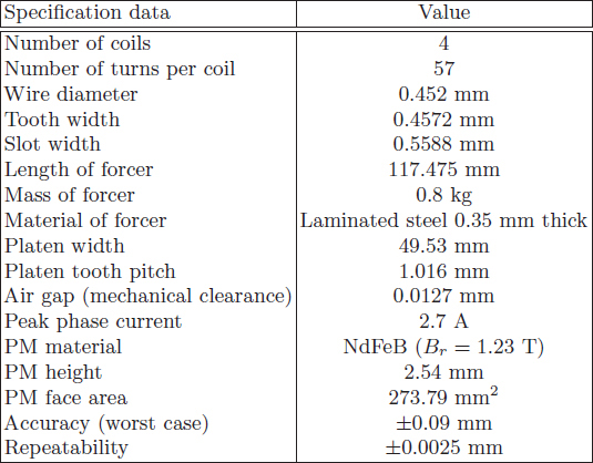
Table 5.1. Design data of the tested L20 HLSM manufactured by Parker Hannifin Corporation, Compumotor Division, Rohnert Park, CA, USA [40]
The stepping resolution of the HLSM has no significant influence on the amplitude of both the tangential and normal ripple forces. Both harmonic-added and harmonic-subtracted schemes work equally well in reducing the amplitude of the force ripple. However, in the case of a normal force, there is better improvement when subtracting the 3rd harmonic from the current profile than when adding it. It has also been found that the amplitude of the tangential force ripple increases with the increase in phase current. The relation between them is not so linear as reported [138]. Higher-order harmonics cannot be neglected when the magnetic circuit becomes highly saturated.
Transient performance measurements are focused on the acceleration (startup) and deceleration (braking). The startup tests can simply be done by supplying power to the HLSM and recording the motor’s acceleration. The time interval from the instant at which the power is switched on to the instant at which the HLSM reaches steady-state speed is called the startup setting time. For a typical HLSM, it is about 1 s to reach its steady-state speed at no load. As expected, somewhat longer time will be needed when certain load is applied. The braking time is also inversely proportional to the attached mass.
Case Study 5.1. L20 HLSM
The L20 HLSM manufactured by Parker Hannifin Corporation, Compumotor Division [40] has been tested experimentally. The specification data of the L20 HLSM are given in Table 5.1. Then, its characteristics obtained from measurements have been compared with the FEM and RNA results.
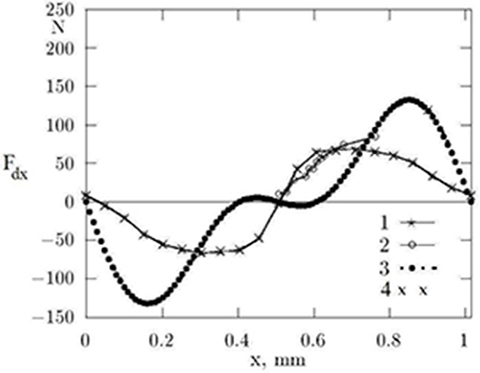
Fig. 5.6. Tangential force versus displacement (when one phase of the motor is fed with 2.7 A current): 1 — FEM, 2 — measurements, 3 — RNA, 4 — Maxwell stress tensor.
The following static characteristics have been considered: (1) static force versus forcer position, and (2) holding force versus peak phase current when only one phase of the HLSM is fed with peak phase current. The results obtained from the FEM, RNA, and measurements are shown in Figs 5.6 and 5.7. It can be seen that the maximum holding force obtained from the FEM, measurements, and RNA are 70 N, 85 N, and 120 N, respectively (Fig. 5.6). The FEM (Coulomb’s approach) results correlate well with the experimental results in the case of static characteristics. The RNA tends to overestimate the force since simplifications have been made to calculate the force.
The instantaneous characteristics of the HLSM refer to the output tangential force versus motor position when the HLSM has been powered up and is reaching its steady state. A set of different excitation current waveforms have been used both in testing and computations. They are pure-sine waves and quasi-sinusoidal waves with 4% and 10% of the 3rd harmonics added, respectively.
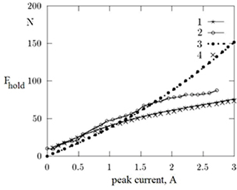
Fig. 5.7. Holding force versus peak current when only one phase is fed. 1 — FEM (Coulomb’s approach), 2 — measurements, 3 — RNA, 4 — FEM (Maxwell stress tensor).

Fig. 5.8. Instantaneous tangential forces versus displacement (when the phase A of the HLSM is driven with pure sine wave and phase B with pure cosine wave). 1 — FEM (Coulomb’s approach), 2 — measurements, 3 — RNA, 4 — FEM (Maxwell stress tensor).

Fig. 5.9. Instantaneous tangential force versus displacement (when 10% of the 3rd harmonic has been injected into the phase current). 1 — FEM (Coulomb’s approach), 2 — measurements, 3 — RNA, 4 — FEM (Maxwell stress tensor).
The results obtained from both the FEM and RNA are then compared with measurements as shown in Figs 5.8 and 5.9. Since the HLSM operated at a constant speed of 0.0508 m/s, the force-time curves could be easily transformed to force-displacement curves. In general, the RNA tends to overestimate the force versus displacement as compared with the measured values, while the virtual work method gives more accurate (although underestimated) results. However, the RNA is a very efficient approach from the computation time point of view.
Fig. 5.10 shows the amplitude of tangential force ripple plotted against the peak current. This has been obtained by calculating the maximum force ripple for each peak value of the excitation current.
Owing to the existence of the PM, there is a strong normal force between the forcer and platen even when the HLSM is unenergized (Fig. 5.11). It can also be seen in Fig. 5.11 that the normal force is very sensitive to the small change in the air gap. The FEM results show that the normal force (Fig. 5.12) almost doubled when the HLSM is energized (peak phase current 2.7 A). In this case, the RNA gives results fairly close to the FEM.
An accurate prediction of forces is necessary not only for motor design purposes but also for predicting the performance of a HLSM drive system. Both the FEM and RNA give the results very close to the test results. The accuracy of the FEM depends much on the discretization of the air gap region while the accuracy of the RNA depends on the evaluation of reluctances. The existence of PMs and toothed structures is the main factor in generating ripple forces. The reduction of ripple forces is necessary to obtain a smooth operation of the motor and minimize audible noise. The force ripple can be suppressed by modifying the input current waveforms. HLSMs with adjustable current profiles offer new techniques of motion control.
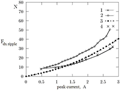
Fig. 5.10. Tangential force ripple amplitude as a function of peak current: 1 — FEM (Coulomb’s approach), 2 — measurements, 3 — RNA, 4 — FEM (Maxwell stress tensor).

Fig. 5.11. Calculated normal force between forcer and platen versus air gap length at current free state: 1 — FEM (Coulomb’s approach), 2 — RNA.
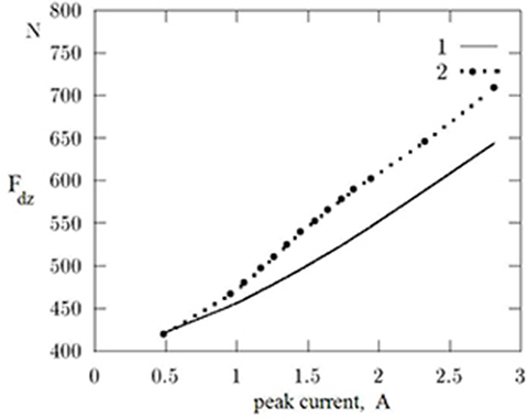
Fig. 5.12. Normal force versus peak current: 1 — FEM (Coulomb’s approach), 2 — RNA.
5.2 Five-Phase Permanent Magnet Linear Synchronous Motors
Although the most popular are three-phase PM LSMs, their five-phase counterparts show some fault tolerance and reduced detent force [211, 213, 215, 220]. Minimization of the detent force reduces the level of vibration, which is very important in precision mechanisms used in a variety of mechatronics systems. In this section, investigations into five-phase tubular PM LSMs (Fig. 5.13) carried out at the Technical University of Opole, Poland, have been presented [207, 208, 209, 210, 213, 230, P214].
Tubular five-phase PMS LSMs can be designed as linear machines with modular armature units and reaction rails assembled with ring-shaped PMs and soft ferromagnetic materials [214, 216, 217]. Modular armature units allows for building a series of five-phase LSMs with different ratings. The longitudinal section of a five-phase tubular PM LSM consisting of one armature module is shown in Fig. 5.16.
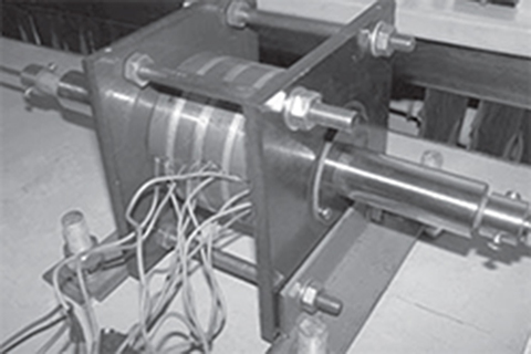
Fig. 5.13. Prototype of a five-phase tubular PM LSM [220].
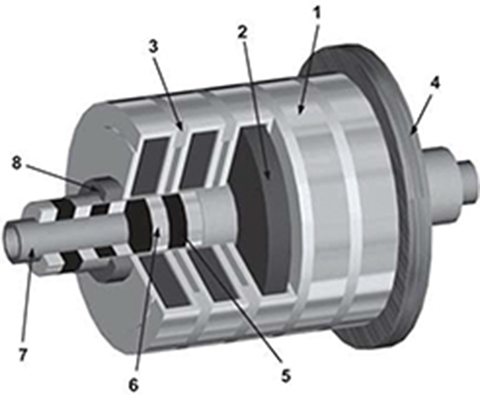
Fig. 5.14. Cutaway view of five-phase tubular PM LSM. 1 — armature segment, 2 — armature coil, 3 — nonferromagnetic ring, 4 — armature cover, 5 — PM, 6 — ferromagnetic ring, 7 — nonferromagnetic tube, 8 — linear slide bearing.
5.2.1 Geometry
The cutaway view of a five-phase tubular PM LSM is shown in Fig. 5.14. The armature coils are magnetically separated. More armature modules can be added to achieve the desired thrust. An axonometric view of a similar flat five-phase PM LSM is shown in Fig. 5.15.
The longitudinal section of a five-phase tubular PM LSM is presented in Fig. 5.16. The reaction rail is assembled of NdFeB 35 PM and mild steel rings. The B-H curve for mild steel is given in Fig. 4.8a [219]. The longitudinal section of a five-phase flat PM LSM is shown in Fig. 5.17.
Flat and tubular five-phase LSMs with the same dimensions have been used for comparative analysis (Figs 5.16 and 5.17). The thrust of the tubular LSM is very close to that of the flat LSM. Dimensions of flat and tubular motors are given in Table 4.1, i.e., dimensions are the same as those of three-phase LSMs discussed in Chapter 4.
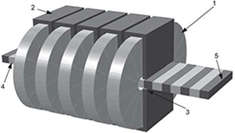
Fig. 5.15. Axonometric view of the flat motor construction. 1 — armature coil, 2 — ferromagnetic core, 3 — tooth of the armature segment, 4 — PM, 5 — flat ferromagnetic bar.

Fig. 5.16. Longitudinal section of five-phase tubular PM LSM. 1 — armature coil, 2 — ferromagnetic core, 3 — tooth of the armature segment, 4 — PM, 5 — ferromagnetic ring.
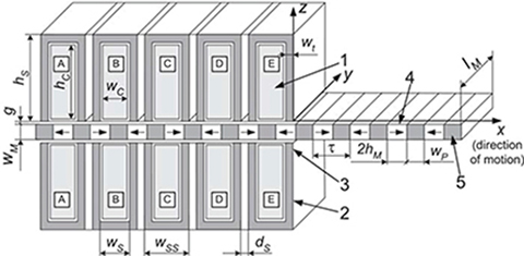
Fig. 5.17. Longitudinal section of five-phase flat PM LSM. 1 — armature coil, 2 — ferromagnetic core, 3 — tooth of the armature segment, 4 — PM, 5 — flat ferromagnetic bar.
The length lM = 48.7 mm (perpendicular to armature laminations, as shown Fig. 5.17) of the flat motor is equal to the mean circumference of the air gap (radius r0 + 0.5 = 15.5 mm) of the tubular LSM (Fig. 5.16).
For proper operation of five-phase motors, the dimensions wss, ds, and τ should meet the following conditions [230]:
where k is the smallest integer for which ds > 0. For main dimensions of five-phase motors as given in Table 4.1, the distance between armature modules amounts to ds = 3 mm.
5.2.2 2D Discretization and Mesh Generation
In the 2D FEM analysis of five-phase LSMs, PDE equations have been solved using the Dirichlet boundary conditions (Fig. 5.18). Only a half of tubular LSM with axial symmetry (Fig. 5.16) can be considered. In FEM modeling, the fine mesh should be dense enough in order to obtain high accuracy of computations (Fig. 5.19).
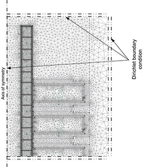
Fig. 5.18. The analyzed area with the Dirichlet boundary conditions.
The most important region in linear motors, as in any other electrical machines, is the air gap g (mechanical clearance) between the armature and reaction rail. This region is limited by lines m and n in Fig. 5.19. A fine mesh must be applied to the discretization of the air gap. There are subdomains between lines k and l in Fig. 5.16, which include one module of the armature. The PMs, mild steel rings, and windings have been discretized with a mesh of different density.
Considering the air gap, there are two and four 3-node elements in the radial direction for coarse and medium-quality meshes. For the finest mesh, seven 6-node elements in the radial direction have been employed. It is necessary to emphasize that the air gap should be divided at least into two rows of elements. This is visible in Fig. 5.19a, between lines m and n.
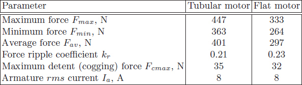
After solution of PDEs, the so called differential parameters, e.g., flux density or integral parameters, such as forces of the magnetic field are obtained. The electromagnetic force (thrust) is the most important integral parameter. In Fig. 5.20, the electromagnetic thrust versus the distance z of the moving reaction rail is shown. Results for coarse, medium, and fine meshes have been compared. Thrusts developed by the flat and tubular five-phase PM LSMs are presented in Table 5.2.
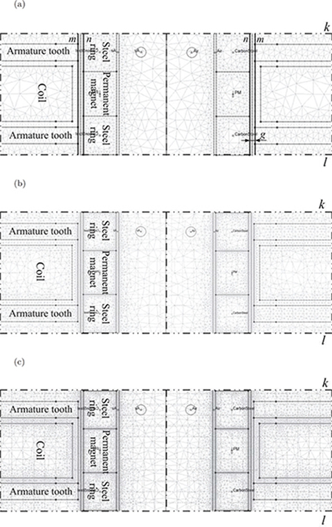
Fig. 5.19. Discretization of a tubular PM LSM using meshes of different density: (a) coarse, (b) medium, (c) fine.
Table 5.2. Electromagnetic thrust under rated (nominal) current for the analyzed prototypes of flat and tubular five-phase PM LSMs
The coefficient of thrust ripple kr is defined by eqn (4.79). The errors in the average force value and thrust ripple coefficient for different mesh densities have been estimated as
Calculation results of the thrust, coefficient of thrust ripple, and errors are given in Table 5.3.

Fig. 5.20. Comparison of force calculation results for different mesh densities.
Table 5.3. Comparison of thrust, coefficient of thrust ripple and errors for different mesh densities (Fig. 5.19)

Table 5.3 shows that further increase in the number of elements of the air gap does not change the average force Fav. Thus, overdiscretization causes longer calculation time without significant improvement in most of the parameters.
In Fig. 5.21, the fine meshes of tubular and flat motors are drawn. For both cases, the air gap region mesh density is higher than the mesh density of other regions. A dense mesh in the air gap region is necessary to obtain more accurate computation results of electromagnetic forces. Maxwell’s stress tensor should be integrated near the ferromagnetic edges.
5.2.3 2D Electromagnetic Field Analysis
Figs 5.22 and 5.23 show the calculated 2D magnetic field distribution, in particular, magnetic flux lines. The 2D field distribution has been obtained for two load angles: δ = 0 (Fig. 5.22) and maximum angle δ = 90° (Fig. 5.23). The motor draws maximum armature current Ia = 8 A (Table 5.2). The various gray shades visualize different values of the magnetic flux density. In the top right corners of Figs 5.22b and 5.23b, the five-phase system of currents is shown. The value of the armature current corresponding to the calculated time instant can be obtained as a projection of the current phasor onto the vertical axis in the complex plane. Under the same supply and loading, the flux density distributions are similar for both flat and tubular LSMs. However, for the flat motor (Figs. 5.22b and 5.23b), the magnetic flux density distribution in the armature modules is more homogenous as compared with tubular motor (Figs. 5.22a and 5.23a). In the tubular motor, the highest values of the magnetic flux density are in the armature teeth. This is due to variation of the cross section of the teeth with the radius of the cylindrical module. The magnetic flux that links the coil turns is a nonlinear function of the armature current. The saturation level increases with the armature current Ia.
Recommendations for sizing procedure can be made on the basis of the 2D magnetic field distributions in both tubular and flat LSMs. To obtain parameters of a flat LSM similar to those of a tubular LSM, the length lM of the flat motor shall be equal to the circumference of the air gap of the tubular motor. The magnetic saturation effects are less evident in the flat motor.
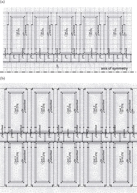
Fig. 5.21. Discretization mesh of five-phase PM LSMs: (a) tubular motor, (b) flat motor.
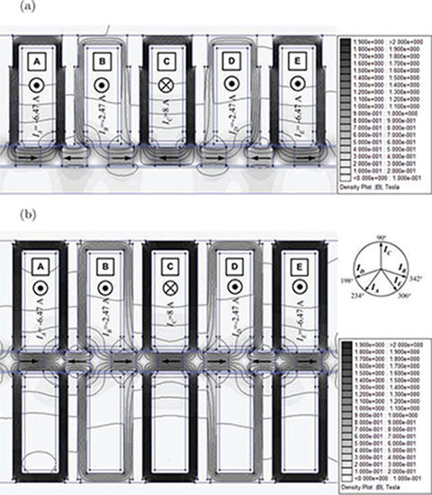
Fig. 5.22. Magnetic field distribution at load angle δ = 0: (a) tubular LSM, (b) flat LSM.
5.2.4 3D Electromagnetic Field Analysis
For better accuracy of computations, a flat PM LSM (Fig. 5.15) should be analyzed in 3D. The 3D field distribution has been obtained for the current system shown in Fig. 5.23. The 3D magnetic flux distribution in the armature and reaction rail of the five-phase PM LSM is presented in Fig. 5.24. The highest concentration of flux lines is observed in the first and the fourth segment of the armature (on the left side of the motor). In PM, the magnetic field is rather homogenous. Inside the ferromagnetic pieces of bars located between PMs, the highest magnetic flux density is observed in the corners.
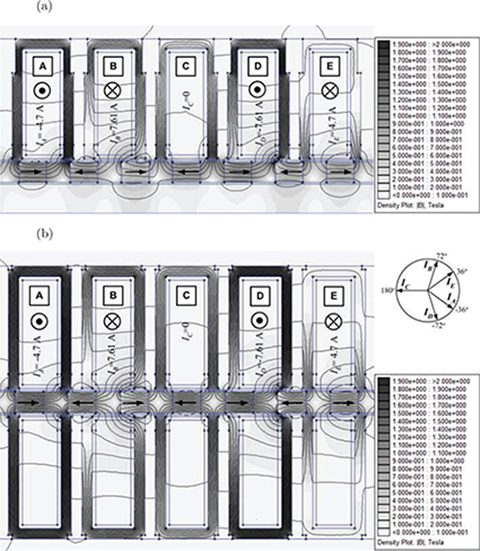
Fig. 5.23. Magnetic field distribution at maximum load angle δ = 90°: (a) tubular LSM, (b) flat LSM.
The field integral parameters have also been found from the 3D analysis. The most important is thrust. According to the 3D analysis, the electromagnetic thrust F = 282 N, while according to the 2D analysis, the thrust F = 304 N. The width lM = 48.7 mm is sufficient enough to perform only the 2D analysis. However, if this dimension is smaller, 3D analysis should be executed.
The distribution of the magnetic flux density modulus has been plotted in Fig. 5.25. The field distribution in the portion of full region in the xy plane inside the ferromagnetic casing of coil A has been chosen (Fig. 5.17). Arrows represent the flux density vectors. The 3D behavior of the magnetic field distribution is clearly visible. The electromagnetic thrust arises from the magnetic energy stored in the air gap (Fig. 5.25). The field analysis allows for prediction of the magnetic flux polarity in all parts of the reaction rail.
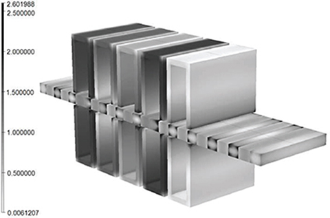
Fig. 5.24. 3D field distribution in a five-phase flat PM LSM.
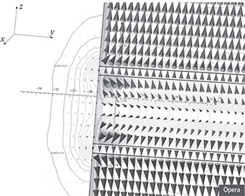
Fig. 5.25. Magnetic flux density distribution in the air gap.
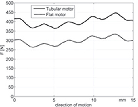
Fig. 5.26. Electromagnetic thrust developed by five-phase LSM versus position of the reaction rail at δ = 90°.

Fig. 5.27. Comparison of the results obtained from 2D and 3D FEM analysis for: (a) tubular LSM, (b) flat LSM.
5.2.5 Electromagnetic Thrust and Thrust Ripple
The most important integral parameter, i.e., the thrust plotted against the position of the reaction rail at armature current corresponding to δ = 90°, is shown in Figs 5.26 and 5.27. The thrust ripple produced by the five-phase LSM is much lower than that in the case of the three-phase motor (Chapter 4). In general, tubular LSMs with the same phase number m1 as flat LSMs are characterized by higher developed thrust (20% to 30%) than flat LSMs (Fig. 5.26). However, the waveforms of the thrust as functions of the reaction rail position are similar for both tubular and flat LSMs.
The difference between the results obtained from 3D and 2D FEM analysis is shown in Fig. 5.27. The 2D analysis gives higher electromagnetic thrust than the 3D analysis. The main reason is that the leakage flux in the end regions is included in the 3D FEM analysis. On the other hand, the fine mesh used in the 2D simulation cannot be implemented in the 3D analysis because of the unacceptably long time of computations.
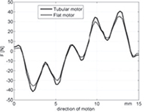
Fig. 5.28. Detent force produced by five-phase PM LSM.
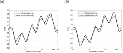
Fig. 5.29. Comparison of detent thrust calculated on the basis of 2D and 3D FEM analysis for (a) tubular LSM, (b) flat LSM.
To obtain the detent force, the FEM analysis of zero armature current Ia = 0 has been performed. The average and maximum force increases with the PM and ferromagnetic ring thickness. For dimensions shown in Table 4.1, the detent force for flat and tubular LSM is nearly the same (Fig. 5.28). The highest value of the detent force is for z = 2.5 mm and z = 13 mm, i.e., nearly 40 N (Figs. 5.28 and 5.29), which is approximately equal to 10% of the thrust. Although, the detent force is significant, the tubular construction is more economical due its higher developed thrust.
The detent force in turn affects the thrust. The number of maxima and minima in detent force waveforms depends on the number of phases (Figs. 4.15 and 5.28). The trust obtained from the 2D FEM analysis (Fig. 5.30) differs from that obtained from the 3D analysis (Fig. 5.31). It is especially visible in the case of the tubular LSM (Fig. 5.31a). This is due to the coarse dis-cretization of the air gap (mechanical clearance) using tetrahedral elements. Considering also CPU time, the user of the 3D FEM software is forced to assume an insufficient number of elements of the mesh.

Fig. 5.30. Electromagnetic force of five-phase LSM versus position of the reaction rail at δ = 0.

Fig. 5.31. Electromagnetic force calculated on the basis of the 3D FEM at δ = 0 for (a) tubular PM LSM, (b) flat PM LSM.
5.2.6 Experimental Verification
Magnetic Flux Density Distribution
The magnetic flux density distribution at the active surfaces of the armature core and reaction rail has been verified experimentally. Since it is difficult to measure the flux density in the air gap, the magnetic fields excited by the reaction rail (PMs) and the armature (input currents) have been measured separately. The field distribution has been measured along the z-axis.
To verify the distribution of the magnetic flux density excited by PMs, the segment AA‘ of the reaction rail without the armature has been considered (Fig. 5.32). The calculated components Bz and Br have been compared with the test results (Fig. 5.33). In the case of the distribution of tangential component Bz, the end effects are not significant (Fig. 5.33a). The first maximum of Bz is about 12% lower than the next one. In the case of the distribution of radial component Br, the maximum values, as expected, are observed near the edges of the ferromagnetic rings (Fig. 5.33b).
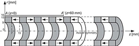
Fig. 5.32. Zone AA‘ of the reaction rail of tubular PM LSM.
The calculated magnetic flux density distribution excited by the armature winding of the tubular LSM without the reaction rail has also been compared with the test results. Only selected coils have been excited.
(a) Coil 1 (Fig. 5.34) has been energized with Ia = 4 A, MMF = 1080 Aturns. The calculated tangential component Bz of the magnetic flux density distribution along the z-axis of symmetry (zone BB‘ as shown in Fig. 5.34) is compared with the test results in Fig. 5.35a).
(b) Coil 3 (Fig. 5.34) has been energized with Ia = 4 A, MMF = 1080 Aturns. The flux density values were measured along the CC‘ zone (Fig. 5.34). The tangential component Bz distribution is given in Fig. 5.35b. Owing to the axial symmetry of the armature, the radial (normal) component Br is equal to zero.
(c) Two coils 1 and 3 (Fig. 5.34) have been energized with the same currents Ia = 4 A. Distributions of the magnetic flux density components Br and Bz are plotted in Fig. 5.36. However, the maximum values of tangential components Bz are nearly twice the maximum values of the radial component Br. The calculated magnetic flux density distributions have been compared with test results within the segment DD‘, which is situated close to the active surface of the armature.

Fig. 5.33. Magnetic flux density components along the AA‘ zone of the reaction rail: (a) tangential component Bz; (b) radial (normal) component Br.
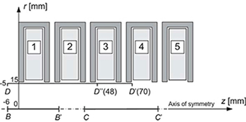
Fig. 5.34. Auxiliary sketch showing location of measurement zones.
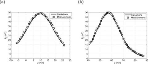
Fig. 5.35. Distribution of tangential component Bz of the flux density at Ia = 4 A: (a) along BB‘ zone with coil 1 being energized; b) along CC‘ zone with coil 3 being energized.
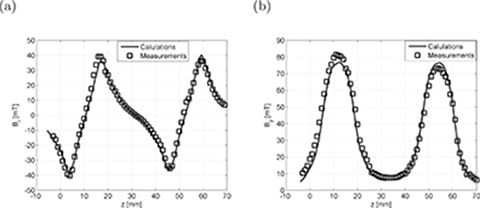
Fig. 5.36. Distribution of magnetic flux density along DD‘ zone at Ia = 4 A in coils 1 and 3: (a) radial component Br, (b) tangential component Bz.
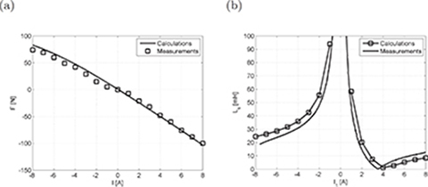
Fig. 5.37. Comparison of measured and calculated integral parameters in the case of reaction rail moved from the central position: (a) thrust, (b) inductance.
Thrust and Inductance
In Fig. 5.37a the electromagnetic thrust is plotted against the armature current when the coil 1 is energized. Fig. 5.37b shows the inductance of coil 1 versus current. Calculations have been compared with test results. The reaction rail has not been positioned in the center of the armature system. In the central position, the armature and reaction rail symmetry axes normal to the active surfaces coincide. Assuming symmetry axis at z = 0, the reaction rail symmetry axis normal to its active surface has been moved to z = 7.5 mm.
5.3 Tubular Linear Reluctance Motors
A tubular linear reluctance motor (LRM) belongs to the group of cyclic actuators with oscillating movement of its movable parts (reaction rails) [27], [160]. So far, reaction rails have been assembled of solid ferromagnetic rods or cylinders [27, 117].
In this section, a laminated silicon steel reaction rail has been proposed. The effects of nonlinearity and laminations on the magnetic field distribution and integral parameters of tubular LSMs have been investigated.
In the case of coreless armature winding (open magnetic system) of a tubular LRM, the traveling magnetic field is generated in the z-direction (Fig. 5.38) by a system of coils. The tubular armature consists of solenoid-type concentrated-parameter coils that constitute a three-phase winding.

Fig. 5.38. Tubular LRM with coreless armature system and the reaction rail. 1 — armature coils, 2 — laminated stack, 3 — spring.
The armature with ferromagnetic core (closed magnetic system) has also been considered. A simplified computer-generated 3D image of a tubular LRM with the armature ferromagnetic core is shown in Fig. 5.39. The external part of the armature core consists of a laminated ferromagnetic cylinder and end disks. The thickness of the cylinder and end disks is dk. In the analysis of the electromagnetic field, the air gaps between the cylinder and end disks have been neglected.
Poisson’s equation (4.4) for the tubular LRM can be written in the following form: [208, 209, 210, 213, 215, 249]
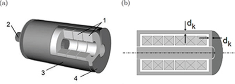
Fig. 5.39. Tubular LRM with ferromagnetic armature core (a) 3D computer created image, (b) longitudinal section. 1 — coils, 2 — moving rod (runner), 3 — ferromagnetic housing, 4 — ferromagnetic end disks.
in which A is the magnetic vector potential, v is the velocity of the magnetic field excited by the current density J, and σ is the electric conductivity. For slow time-varying magnetic fields (slowly moving raction rail), the second term σ(v × ∇ × A − ∂A/∂t) on the right-hand side of enq (5.23) vanishes.
To include the anisotropy of laminated reaction rail, 3D FEM analysis must be used. Thus, the application of magnetic scalar potentials is more convenient and efficient in the analysis of the spatial field than magnetic vector potential. The so-called total magnetic scalar potential ψ and reduced scalar potential φ have been employed, i.e.,
Case Study 5.2. 3D FEM Magnetic Field Analysis in tubular LRM
The 3D FEM analysis have been performed using the Opera-3d commercial package [25, 162]. Steady-state characteristics and electromagnetic parameters of LRMs have been found using the FEMM 4.0 package [144].
In the analyzed LRM, the length of the armature winding is 160 mm. The outside and inside diameters of coils are do = 85 mm and di = 39 mm, respectively. The reaction rail is stacked of silicon steel sheets and inserted in a nonferromagnetic tube with its inside diameter d = 29 mm. Thus, the nonferromagnetic air gap between the armature wires and the ferromagnetic core of the reaction rail is g = 5 mm. The mass of the reaction rail is 1.05 kg, and its length is 190 mm. The air gap between the armature end disks and the reaction rail is 2 mm.
The number of turns per phase is N = 2400 both for the coreless armature and armature with ferromagnetic core. The reaction rail and armature core are made of EP470-50A silicon steel [205, 206]. Since the magnetic circuit is laminated both axially and radially (Fig. 5.38), the electromagnetic field analysis must include anisotropy.
Magnetic Field in Laminated Reaction Rail
It has been assumed [205, 206] that the magnetization curve B-H of the reaction rail in the direction of motion (z-axis) is typical, such as that given in catalogues of electrical sheet steels. The B-H curve in the direction perpendicular to the plane of laminations (Fig. 5.38b) is extremely different from that in the z-direction. Manufacturers of electrical sheet steels normally do not provide this B-H curve. However, if the thickness of laminations and difference between magnetic permeabilities in both directions are known, the magnetization curve in the direction perpendicular to the plane of laminations can be reconstructed, e.g., [207].
The 3D FEM mesh contains over 280 000 elements. The anisotropy effect is especially visible in the nonsaturated core (Fig. 5.40a), when the armature current is small, e.g., Ia = 1.0 A, and the reaction rail is in the central position. For comparison, the computation results for the isotropic core (solid steel) of reaction rail are presented in Fig. 5.40b. The “step” corners of the anisotropic stack are more saturated than those of the isotropic stack, even for small armature current Ia = 1.0 A (Fig. 5.40b). Increase in the armature current to Ia = 8.0 A causes the reaction rail to saturate (Fig. 5.41). However, at each end of the reaction rail, the inner area of the cross section remains unsaturated.
Magnetic Field in Assembled LRM
A tubular LRM with armature furnished with ferromagnetic core is shown in Fig. 5.39. The armature winding is enclosed with a laminated silicon steel core. To simplify the analysis, eddy currents in the laminated armature core have been neglected. Calculations have been executed for quantitative changes in the armature current and the thickness dk of the stator cylindrical core (Fig. 5.39) and for various axial positions of the reaction rail.
The ferromagnetic cylindrical core with its thickness dk = 1.5 mm (Fig. 5.42b) is rather a magnetic shield for armature winding than a part of the magnetic circuit. For small armature current Ia = 1.0 A, the average magnetic flux density value in the reaction rail is 0.75 T in the case of coreless armature winding (Fig. 5.42a) and 0.95 T in the case of armature winding with ferromagnetic core (Fig. 5.42b).
The shielding effect is also visible in Fig. 5.43 where the armature winding is energized with high armature current Ia = 8 A. The thin cylindrical ferromagnetic core (external part of the armature magnetic circuit) becomes highly saturated. Because of high-level of saturation of the armature core (Fig. 5.43), the magnetic flux distribution in the reaction rail is almost the same for coreless armature winding and armature winding with ferromagnetic core. The average magnetic flux density value in the reaction rail is nearly 1.9 T. However, in the case of the armature with ferromagnetic core, the magnetic flux is forced to concentrate in the edges of the armature core (Fig. 5.43b).
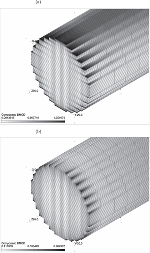
Fig. 5.40. 3D magnetic flux density map for (a) anisotropic reaction rail stacked of laminations, (b) isotropic reaction rail made of solid steel.
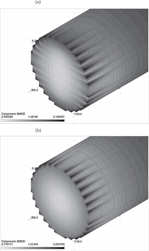
Fig. 5.41. Map of the modulus of the magnetic flux density for saturated reaction rail: (a) anisotropic; (b) isotropic.
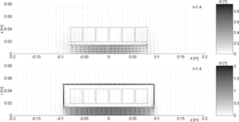
Fig. 5.42. Magnetic flux distribution in longitudinal section for small armature current (Ia = 1 A): (a) coreless armature winding; (b) armature winding with ferromagnetic core.

Fig. 5.43. Flux density distribution for the saturated circuit (I = 8 A): (a) open magnetic system; (b) closed magnetic system.
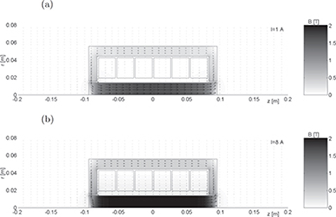
Fig. 5.44. Magnetic flux density distribution in the case of thick cylindrical part of the armature magnetic circuit at (a) Ia = 1.0 A, (b) Ia = 8.0 A.
When the external cylindrical part of the armature magnetic circuit is relatively thick (dk = 12 mm), the magnetic flux distribution for coreless armature system and armature winding with ferromagnetic core considerably differ from each other. It is especially visible for high value of the armature current Ia = 8 A (Fig. 5.44b). The magnetic flux density in the armature winding area is greater than that in the coreless armature system (Fig. 5.43a). Even for a small value Ia = 1.0 A of the armature current, the maximum values of the flux density in the armature system with ferromagnetic core are nearly twice greater, i.e., B = 1.0 to 1.5 T (Fig. 5.44a) than those in the case of coreless armature winding (Fig. 5.42a).
More interesting is the behavior of the magnetic flux when the reaction rail is not in the armature central position. For example, if at Ia = 8.0 A half of the reaction rail is outside the armature system, the smaller portion of the reaction rail covered by the armature magnetic circuit becomes highly saturated (Fig. 5.45a). The reaction rail is more saturated in the case of the armature with ferromagnetic core (Fig. 5.45b) than in the case of coreless armature.
Experimental Verification
The distribution of Bz and Br components along the z-axis obtained from calculations and measurements are plotted in Figs. 5.46 and 5.47. Measurements have been performed only for the tubular LRM with coreless armature system for the reaction rail positioned at z = 80 mm with respect to the central position. A good agreement between calculation and test results confirms the correctness of computer simulations.

Fig. 5.45. Magnetic flux distribution at Ia = 8 A and reaction rail not positioned in the center of the armature system: (a) coreless armature winding; (b) armature winding with ferromagnetic core.
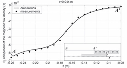
Fig. 5.46. Distribution of radial component Br of magnetic flux density along the zone AA‘.

Fig. 5.47. Distribution of tangential component Bz of magnetic flux density along the zone BB‘.
5.4 Linear Oscillatory Actuators
The linear oscillatory actuator (LOA) of the reluctance type belongs to the group of short-stroke actuators [68, 160]. Their construction is very simple(Fig. 5.48): the stationary part with coils is fed from an a.c. source, while the movable part constitutes a ferromagnetic bar. LOAs convert electrical energy into sustained short-stroke reciprocating motion [252]. Applications include, but are not limited to, reciprocating compressors, vibrators, pumps, shuttles of weaving looms, electric hammers, etc.
In an LOA, the magnetic energy depends on the position of the moving bar. The energy takes maximum value when the moving bar is in the center of the stationary part (z = 0), as shown in Fig. 5.48. As the bar moves left or right (z ≠ 0), the magnetic energy decreases. A change in energy produces the electromagnetic force acting on the moving bar.
The RLC circuit consisting of the stationary coil and series capacitor is in resonance when the center of the moving ferromagnetic bar approaches the edge of the coil. At this instant, the current in the coil abruptly increases and high electromagnetic force pulls the bar into the center of the coil and further toward the opposite edge of the coil. The resonance occurs again and the cycle is repeated.
LOAs have been widely studied using the circuital approach, e.g., [31, 141, 160], and the FEM, e.g., [252]. This section is devoted to electromagnetic field analysis, integral parameters, and calculations of dynamic performance characteristics of LOAs.
5.4.1 2D Electromagnetic Field Analysis
The electromagnetic field analysis in a LOA (Fig. 5.48) can be brought to the analysis of a magnetically open problem [231, 204, 250]. In general, the problem should be analyzed using a method that does not require any limitation of the calculated area, e.g. boundary integral method (BIM) [204, 250].
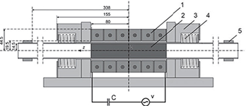
Fig. 5.48. Longitudinal section of a LOA. 1 — stationary coil, 2 — moving bar, 3 — housing, 4 — spring, 5 — limiter.
Since the magnetic circuit is open (Fig. 5.48), the magnetic flux density in each portion of the magnetic circuit is relatively low. When the mechanical frequency of the moving bar is low (2 to 3 Hz), the displacement currents and eddy-current losses in conductive parts of an LOA can be neglected. With these simplifications, the electromagnetic field is governed by eqn (5.23), in which σ(v × ∇ × A − ∂A/∂t) = 0
For axial symmetry of the LOA, the electromagnetic field can be described by the so-called reduced scalar potential φ, which depends on the angular component Aφ of the magnetic vector potential A and the radius r (the distance between source and field point) i.e., φ = Aφr. Thus
See also eqn (5.24). On the basis of the B-H curve, the relative magnetic permeability μr of the moving bar has been determined. The tangential Bz and radial Br components of the magnetic flux density B have been calculated as
To obtain the reliable values of the magnetic flux density in the vicinity of the stationary part, the dimensions of the investigated region must be at least four times greater than the longest dimension of the LOA [204].
5.4.2 Magnetic Flux, Force, and Inductance
The inductance of the stationary coil can be found either from the total energy of the magnetic field stored in the coil or from the magnetic flux Ψ linked with the coil. The magnetic energy is expressed by eqn (4.33), and the linkage flux by eqn (4.16). When the system is unsaturated, the average total inductance of the stationary coil is expressed by eqn (4.30), and when the system comes into saturation, it is convenient to use eqn (4.18).
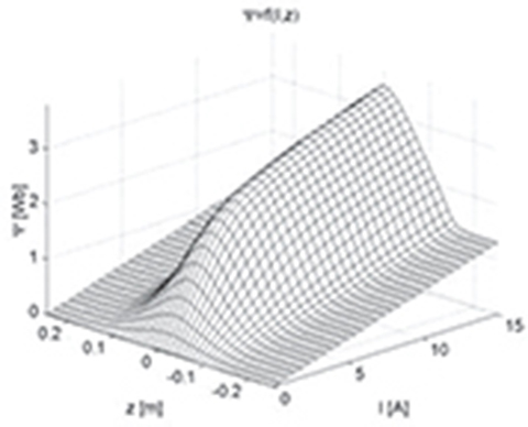
Fig. 5.49. Distribution of magnetic flux linkage as a function of input current and position of moving bar.

Fig. 5.50. Dynamic inductance of the coil as a function of input current and position of moving bar.
As known, the magnetic flux Ψ linking the coil turns depends on the input current. For the LOA shown in Fig. 5.48 and input current exceeding I = 5 A, the function Ψ = f(I) plotted in Fig. 5.49 is strongly nonlinear. For I ≥ 10 A, the system is saturated, and the flux Ψ minimally changes with the current I.
For the position z > 0.12 m of the moving bar, the magnetic flux is practically independent of z. The moving bar is outside the stationary coil, and the coil behaves as an air-cored coil. Thus, the flux linkage is a linear function of the current I.
It is evident from Fig. 5.50 that the inductance L of the stationary coil decreases as the current increases. For the dead zone of the bar (in the middle of the stationary coil), the inductance decreases from Lmax = 0.55 H to Lmin = 0.1 H as the current increases from 1.0 to 15.0 A.
When the current is greater than 2.0 A, the moving bar gets slightly saturated and the inductance drops somewhat. The bottom margin of the inductance (for the current resonance) is nearly 0.1 H.
The electromagnetic force acting on the moving bar as a function of the input current and bar position is plotted in Fig. 5.51. The direction of the electromagnetic force depends on the position of the moving bar, i.e. for z < 0, the force is positive, and for z > 0, the force in negative.
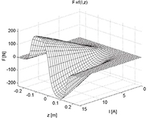
Fig. 5.51. Electromagnetic force as a function of input current and position of moving bar.
Case Study 5.3. LOA Dynamics
An LOA can be desribed by the following equations:
electric balance equation
mechanical balance equation
in which v(t) is the input voltage, L(z, i) is the inductance of the stationary coil, Ψ(z, i) is the magnetic flux linked with the stationary coil, C is the series capacitance in the stationary coil circuit, R is the stationary coil resistance, m is the mass of moving bar including load, Dv is the damping (friction) constant, f = ∂W'/∂z is the electromagnetic force calculated on the basis of magnetic coenergy W', fs = ks(z0 − z) is the spring force, and ks is the spring constant (stiffness). See also eqns (1.28) amd (1.29).
To study the dynamic behavior of the LOA, it has been assumed that
(a) the moving bar position changes from z(t) = 0 to |z(t)| = 0.188 m;
(b) the coefficients in eqn (5.28) are m = 1.05 kg, kfr = 2 Ns/m, ks = 2 kN/m;
(c) electrical parameters in eqn (5.27) are R = 8.5 Ω, C = 100 μF, z0 = 0.188 m.
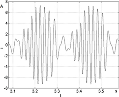
Fig. 5.52. Computed waveform of the current in stationary coil at v = 50 V.
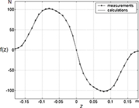
Fig. 5.53. Static force acting on moving bar at I = 8.0 A.
A direct solution to eqns (5.27) and (5.28) is not possible without physical simplifications. Eqns (5.27) and (5.28) have been solved using Matlab and toolboxes PDE and Simulink [167]). After computing the integral parameters of the magnetic field, the combined kinetic and electric field equations have been solved simultaneously. The computed results for v = 50 V are given in Fig. 5.52.
Experimental verifications of computer simulations have been done for the moving 160-mm long steel bar. The mass of the bar is 1.05 kg. The stationary winding consists of six coils connected in series, each wound with 400 turns. The outside and inside diameters of each coil are 85 mm and 39 mm, respectively.
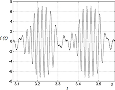
Fig. 5.54. Experimental results for the stator current, v = 50 V.
The force has been measured keeping constant the value of the current. The static force as a function of the moving bar position is plotted in Fig. 5.53.
The electromagnetic force as a function of time at v = 50 V is plotted in Fig. 5.54. Compare Fig. 5.54 with Fig. 5.52. The peak forces are almost the same.
Examples
Example 5.1
An HLSM has two poles (2p = 2) and n = 10 slots per pole. Dimensions of the magnetic circuit are as follows
slot width b = 0.56 mm
tooth width c = 0.46 mm
air gap g = 0.014 mm
length of the forcer stack (perpendicular to the direction of motion) Li = 12 mm
width of pole (along the platen) wp = 22 mm
The stacking factor ki = 0.97. Find the variation of the air gap permeance Gt(x) and variation of the tangential force per pole Fdx(Bg, x) for the air gap magnetic flux density Bg = 0.25 T, 0.5 T, and 0.75 T.
Solution
Pole pitch of the forcer
Maximum air gap permeance according to eqn (5.10)
Mnimum air gap permeance according to eqn (5.11)
Variation of air gap permeance with the x-axis is expressed by eqn (5.9) and plotted in Fig. 5.55.

Fig. 5.55. Variation of air gap permeance with the x-axis.
The first derivative of permeance with respect to the x-axis is given by eqn (5.12), i.e.,

Fig. 5.56. Variation of tangential force Fdx with the x-axis at the air gap magnetic flux density Bg = 0.25 T, 0.5 T, and 0.25 T.
Putting, e.g., x = 0.0008 m, the first derivative ∂Gt/∂x = 0.00138 H/m. The magnetic flux
Putting, e.g., Bg = 0.75 T, the magnetic flux Φ = 1.28 × 10⁻⁴ Wb.
The distribution of the tangential forces Fdx is calculated with the aid of eqn (5.18). This force for three values of air gap magnetic flux density Bg = 0.25 T, 0.5 T, and 0.25 T is plotted against the x-axis in Fig. 5.56. Putting, e.g., Bg = 0.75 T and x = 0.00025 m, the tangential force Fdx = 52.95 N.
Example 5.2
A three-phase PM LSM has s1 = 60 slots and 2p = 10 poles. The armature winding is Y-connected and fed with V1L = 400 V rms (line-to-line). The linear synchronous speed is vs3 = 8 m/s, the rated (nominal) thrust is Fx = 1200 N, and the efficiency × power factor product is η cos φ = 0.68.
Redesign this three-phase LSM into a five-phase motor assuming that (a) the number of slots per pole per phase is the same, (b) the output power is the same, (c) the η cos φ product is the same, and (d) the phase windings are Y-connected.
Solution
(a) Three-phase motor
The number of slots per pole per phase
must be kept the same for both three-phase and five-phase motors. The number of slots per pole
Output power
Phase voltage
Armature current of three-phase motor
(b) Five-phase motor
Armature current of five-phase motor
For five-phase motor the number of poles must be changed because the armature core is the same (60 slots) and, according to assumption (a), the number of slots per pole per phase must be the same (q1 = 2).
The number of pole pairs of five-phase motor
The number of slots per pole
The pole pitch of five-phase motor increases approximately in proportion to Q15/Q13 = 10/6, so that the linear speed
The thrust of five-phase motor
For constant output power (approximately for constant input power), the current of five-phase motor is reduced, the speed increases (assuming q1 = 2 = const), and the thrust decreases.
Suppose that the armature current of both 3-phase and 5-phase motors is the same, i.e., Ia5 = Ia3 = 20.38 A. The output power of five-phase motor at the same value of η cos φ = 0.68 product is
The thrust for the same armature current and increased linear speed
The thrust for the same pole pitch (linear speed vs5 = vs3 = 8 m/s)
If the current and pole pitch are the same, the thrust of five-phase motor increases.
Example 5.3
Consider a three-phase tubular LSM as in Example 4.3. Assuming the same dimensions of all parts (Fig. 4.28), the same peak current Im = 31.4 A (Fig. 5.57), and the same load angle δ = 90°, find the magnetic field distribution and integral parameters of a five-phase tubular LSM using the FEM approach. Material parameters and boundary conditions are the same as in Example 4.1. The thrust should be calculated as a function of the the reaction rail position in the interval 0 ≤ z ≤ 20 mm.
Solution
In the case of five-phase construction, the distance ds between segments should be recalculated with the aid of eqn (4.78). For suitable distance between segments, i.e.,
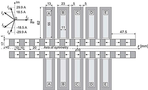
Fig. 5.57. Dimensions of the analyzed five-phase tubular PM LSM and current phasor diagram. The system of the armature currents for z = 0 and δ = 90° is shown in the left top corner.
the coefficient k (Section 4.4) have been assumed k = 2. To keep the same load angle δ = 90° for the whole range of reaction rail movement, the current waveforms must be functions of the reaction rail position. Thus, the system of 5-phase currents is expressed as
For dimensions as in Fig. 5.57, the thrust is determined on the basis of the magnetic field analysis, as an integral parameter. The magnetic field distribution is calculated for several positions of the reaction rail. The magnetic field distribution for two positions (z = 6 mm and z = 16 mm) of the reaction rail is plotted in Fig. 5.58.

Fig. 5.58. Magnetic field distribution at load angle δ = 90° for: (a) z = 6 mm (minimum thrust), (b) z = 16 mm maximum thrust).
The minimum value of the thrust is for z = 6 mm. For z = 16 mm the thrust takes the maximum value. In both cases the highest concentration of magnetic flux lines is in the area of armature teeth.
In the case of three-phase LSM, the thrust (Fig. 5.59) changes from 680 N up to 930 N depending on the position of the reaction rail. The thrust developed by the five-phase LSM is approximately 1.67 higher than that developed by the three-phase motor (Fig. 5.59). This is becuase phase currents of both motors have been assumed the same.
The five-phase LSM produces relatively low thrust ripple (kr = 0.164), approximately 50% lower than the thrust ripple of the three-phase motor (kr = 0.306).

Fig. 5.59. Maximum thrust at δ = 90° versus the reaction rail position.