Chapter 1

What is a loudspeaker?

1.1 A brief look at the concept

Before answering the question posed by the title of this chapter, perhaps we had better begin with the question “What is sound?” According to Fahy¹ “sound may be defined as a time-varying disturbance of the density of a fluid from its equilibrium value, which is accompanied by a proportional local pressure, and is associated with small oscillatory movements of the fluid particles”. The difference between the equilibrium (static) pressure and the local, oscillating pressure is known as the sound pressure.

Normally, for human beings, the fluid in which sound propagates is air, which is heavier than most people think – it has a mass of about 1.2 kg per cubic metre at a temperature of 20 degrees C at sea level. It is also interesting to note that sound propagation in air is by no means typical of its propagation in all substances, especially in that the speed that sound propagates in air is relatively slow, and is constant for all frequencies. For music lovers, this latter fact is quite fortunate, because it would be hard to enjoy a musical performance at the back of a concert hall if the notes arrived jumbled-up, with the harmonics arriving before the fundamentals, or vice versa. Conversely, as we shall see later, most of the materials from which loudspeakers are made do not pass all frequencies at the same speed of sound, a fact which can, at times, make design work rather complicated.

The speed of sound in air is about 343 metres per second (m/s or ms−1) at 20 degrees C and varies proportionally with temperature at the rate of about 0.6 m/s for every degree Kelvin. (In fact, the speed of sound in air is only dependent upon temperature, because the changes that would occur due to changes in atmospheric pressure are equal and opposite to the accompanying changes in density, and the two serve to cancel each other out). Air therefore has some clearly defined characteristic properties, and our perception of sound in general, and music in particular, has developed around these characteristic properties.

The job of a loudspeaker is to set up vibrations in the air which are acoustic representations of the waveforms of the electrical signals that are being supplied to the input terminals. A loudspeaker is therefore an electro-mechanico-acoustic transducer. Loudspeakers transform the electrical drive signals into mechanical movements which, normally via a vibrating diaphragm, couple those vibrations to the air and thus propagate acoustic waves. Once these acoustic waves are perceived by the ear, we experience a sensation of sound.

To a casual observer, a typical moving coil loudspeaker (or ‘driver’ if you wish to restrict the use of ‘loudspeaker’ to an entire system) seems to be a simple enough device. There is a wire ‘voice-coil’ in a magnetic field. The coil is wound on a cylindrical former which is connected to a cardboard cone, and the whole thing is held together by a metal or plastic chassis. The varying electrical input gives rise to vibrations in the cone as the electromagnetic field in the voice coil interacts with the static field of the (usually) permanent magnet. The cone thus responds to the electrical input, and there you have it, sound! It is all as simple as that!...... Or is it?

Well, if the aim is to make a sound from a small, portable radio that fits into your pocket, then maybe that concept will just about suffice, but if full frequency range, high fidelity sound is the object of the exercise, then things become fiendishly complicated at an alarming speed. In reality, in order to be able to reproduce the subtle structures of fine musical instruments, loudspeakers have a very difficult task to perform.

1.2 A little history and some background

When Rice and Kellogg² developed the moving coil cone loudspeaker in the early 1920s, [and no; they did not also invent Kellogg's Rice Krispies!] they were already well aware of the complexity of radiating an even frequency balance of sound from such a device. Although Sir Oliver Lodge had patented the concept in 1898 (following on from earlier work by Ernst Werner Siemens in the 1870s at the Siemens company in Germany), it was not until Rice and Kellogg that practical devices began to evolve. Sir Oliver had had no means of electrical amplification – the thermionic valve (or vacuum tube) had still not been invented, and the transistor was not to follow for 50 years. Remarkably, the concept of loudspeakers was worked out from fundamental principles; it was not a case of men playing with bits of wire and cardboard and developing things by trial and error. Indeed, what Rice and Kellogg developed is still the essence of the modern moving coil loudspeaker. Although they lacked the benefit of modern materials and technology, they had the basic principles very well within their understanding, but their goals at the time were not involved with achieving a flat frequency response from below 20 Hz to above 20 kHz at sound pressure levels in excess of 110 dB SPL. Such responses were not required because they did not even have signal sources of such wide bandwidth or dynamic range. It was not until the 1940s that microphones could capture the full frequency range, and the 1950s before it could be delivered commercially to the public via the microgroove, vinyl record.

Prior to 1925, the maximum output available from a radio set was in the order of milliwatts, normally only used for listening via earphones, so the earliest ‘speakers’ only needed to handle a limited frequency range at low power levels. The six inch, rubber surround device of Rice and Kellogg used a powerful electro-magnet (not a permanent magnet), and as it could ‘speak’ to a whole room-full of people, as opposed to just one person at a time via an earpiece, it became known as a loud speaker. The inventers were employed by the General Electric Company, in the USA, and they began by building a mains-driven power amplifier which could supply the then huge power of one watt. This massive increase in the available drive power meant that they no longer needed to rely on resonances and rudimentary horn loading, which typically gave very coloured responses. With a whole watt of amplified power, the stage was set to go for a flatter, cleaner response. The result became the Radiola Model 104, which with its built in power amplifier sold for the then enormous price of 250 US dollars. [So there is nothing new about the concept of self-powered loudspeakers: they began that way!] Marconi later patented the idea of passing the DC supply current through the energising coil of the loudspeaker, to use it instead of the usual, separate smoothing choke to filter out the mains hum from the amplifier. Therefore right from the early days it made sense to put the amplifier and loudspeaker in the same box.

Concurrently with the work going on at General Electric, Paul Voight was busy developing somewhat similar systems at the Edison Bell company. By 1924 he had developed a huge electro-magnet assembly weighing over 35 kg and using 250 watts of energising power. By 1926 he had coupled this to his Tractrix horn, which rejuvenated interest in horn loudspeakers because it enormously improved the sensitivity and acoustic output of the moving coil loudspeakers, and when properly designed did not produce the ‘honk’ sound associated with the older horns. Voight then moved on to use permanent magnets, with up to 3.5 kg of Ticonal and 9 kg of soft iron, paving the way for the permanent magnet devices and the much higher acoustic outputs that we have today.

Gilbert Briggs, the founder of Wharfedale loudspeakers, wrote in his book of 1955³ “It is fairly easy to make a moving-coil loudspeaker to cover 80 to 8,000 cycles [Hz] without serious loss, but to extend the range to 30 cycles in the bass and 15,000 cycles in the extreme top presents quite a few problems. Inefficiency in the bass is due mainly to low radiation resistance, whilst the mass of the vibrating system reduces efficiency in the extreme top”. The problem in the bass was, and still is, that with the cone moving so relatively slowly, the air in contact with it simply keeps moving out of the way, and then returning when the cone direction reverses, so only relatively weak, low efficiency pressure waves are being propagated. The only way to efficiently couple the air to a cone at low frequencies is to either make the cone very big, so that the air cannot get out of the way so easily, or to constrain the air in a gradually flaring horn, mounted directly in front of the diaphragm. Unfortunately, both of these methods can have highly detrimental effects on the high frequency response of the loudspeakers. For a loudspeaker cone to vibrate at 20 kHz it must change direction forty thousand times a second. If the cone has the mass of a big diaphragm needed for the low frequencies, its momentum would be too great to respond to so many rapid accelerations and decelerations without enormous electrical input power – hence the loss of efficiency alluded to by Briggs. Large surfaces are also problematical in terms of the directivity of the high frequency response, but we will come to that later. So, we can now begin to see how life becomes more complicated once we begin to extend the frequency range from 20 Hz to 20 kHz – the requirements for effective radiation become conflicting at the opposing frequency extremes.

The wavelength of a 20 Hz tone in air is about 17 metres, whereas the wavelength at 20 kHz is only 1.7 centimetres, a ratio of 1000 to 1, and for high quality audio applications we want our loudspeakers to produce all the frequencies in-between at a uniform level. We also need them to radiate the same waveforms, differing only in size (but not shape) over a power range of at least 10,000,000,000 to 1 and with no more than one part in a hundred of spurious signals (non-linear distortion). It is a tall order! Indeed, for a single drive unit, it still cannot be achieved at any realistic SPL (sound pressure level) if the full frequency range is required.

1.3 Some other problems

There are also many mechanical concepts which must be considered in loudspeaker design. For example, the more that one pushes on a spring, the more one needs to push in order to make the same change in length. If the force is limited to less than what is necessary to fully compress the spring, equilibrium will be reached where the applied force and the reaction of the spring balance each other. This is useful when we go to bed, because it prevents the suitably chosen springs from bottoming out, and allows the mattress to adapt to our shape yet retain its springiness. The suspension systems of loudspeaker diaphragms are also springs, but they must try to maintain a consistent opposition to movement or they would compress the acoustical output. If, for example, the first volt of input moved the diaphragm x millimetres, and a second volt moved it only 0.8 x mm further, this would be no good for high fidelity, because when we double the voltage we expect to see the same linear increase in motion. Otherwise, the acoustic output would not be linearly following the electrical input signal, and the non-linear movement would introduce distortion. Therefore, to keep the diaphragm well centred, but to still allow it to move linearly with the input signal, suspension systems must be used which do not exhibit a nonlinear restorative force as the drive signal increases, at least not until the rated excursion limit is reached. (However, as we shall see in Chapter 8, certain non-linear loudspeaker characteristics may actually be desirable for musical instrument amplification.) We tend complicate this suspension problem further when we put a loudspeaker drive unit into a box, because the air in the box acts as an additional spring which is also not entirely linear.

Electrically we can also run into similar problems. Whenever an electric current flows through a wire, the wire will heat up. It is also a property of voice coil wires that as they heat up their resistance increases. As the resistance increases, the signal voltage supplied by the amplifier will proportionally drive less current through the coil. So, as the drive force depends on the current flowing through the wire which is immersed in the magnetic field, if that current reduces, the movement of the diaphragm will reduce correspondingly. We therefore can encounter a situation where the amplifier sends out an accurate drive signal voltage, but how the loudspeaker diaphragm responds to it can, depending on level, change with the voice coil temperature and the springiness of both the air and the suspension system. Even the very magnetic field of the permanent magnet, against which the drive force is developed, can be modulated by the magnetic field given rise to by the signal in the voice coil. Notwithstanding, all of these effects, we still need our diaphragm to move exactly as instructed by the drive voltage from the amplifier, because in reality modern amplifiers are usually voltage sources. This is despite the fact that the loudspeaker motor is current driven, and that the voice coil resistance and reactance (together they form the impedance) will not remain constant over the whole of the frequency range.

Clearly, things are beginning to get complicated, and already we have seen problems begin to pile up on each other. The concept of a loudspeaker being simply an electromagnet, coupled to a moveable cone and placed into a box is obviously not going to produce the high fidelity sounds needed for music recording and reproduction. Good loudspeakers are complex devices which depend on the thorough application of some very rigid principles of electroacoustics in order to perform their very complex tasks. In the minds of most people the concept of a loudspeaker, if it exists at all, is usually grossly over-simplified, and unfortunately this is the case even with most professional users of loudspeakers.

Typical loudspeaker systems consisting of one or more vibrating diaphragms, either on one side of a rectangular cabinet or flush mounted into a wall, represent physical systems of sufficient complexity that accurate and reliable predictions of their sound radiation are rare, if not nonexistent, even with the aid of modern computer technology. Despite the fact that we inevitably have to deal with a degree of artistry and subjectivism in the final assessment, at the design and development stages we must stick close to the objective facts. So, to begin to understand the mechanisms of sound radiation it is necessary to establish the means by which a sound ‘signal’ is transported from a source, through the air, and to our ears.

1.4 Some basic facts

As explained in the opening paragraphs of this chapter, acoustic waves are essentially small local changes in the physical properties of the air which propagate through it at a finite speed. The mechanisms involved in the propagation of acoustic waves can be described in a number of different ways, depending upon the particular cause or source of the sound. With conventional loudspeakers that source is the movement of a diaphragm, so it is appropriate here to begin with a description of sound propagation away from a simple moving diaphragm.

1.4.1 Acoustic wave propagation

The process of sound propagation is illustrated in Figure 1.1. For simplicity, the figure depicts a diaphragm mounted in the end of a uniform pipe, the walls of which constrain the acoustic waves to propagate in one dimension only. Before the diaphragm moves (Figure 1.1(a)), the pressure in the pipe is the same everywhere and equal to the static (atmospheric) pressure P₀. As the diaphragm moves forwards (Figure 1.1(b)), it causes the air in contact with it to move, compressing the air adjacent to it and bringing about an increase in the local air pressure and density. The difference between the pressure in the disturbed air and that of the still air in the rest of the pipe gives rise to a force which causes the air to move from the region of high pressure towards the region of low pressure. This process then continues forwards, and the disturbance is seen to propagate away from the source in the form of an acoustic wave. Because air has mass, and hence inertia, it takes a finite time for the disturbance to propagate through the air; a disturbance ‘leaves’ a source and ‘arrives’ at another point in space some time later (Figure 1.1(c)). The rate at which disturbances propagate through the air is known as the speed of sound, which has the symbol ‘c’, and after a time of t seconds, the wave has propagated a distance of x = ct metres. Note, though, that the speed of propagation is not related to the velocity of the diaphragm. In the great tsunami of December 2004, a five metre displacement of the ocean floor caused a tidal wave to travel at over 500 kilometres per hour, a speed much more rapid than that of the displacement which caused it. For most purposes, the speed of sound in air can be considered to be constant, and independent of the particular nature of the disturbance, although as previously stated it does vary with temperature. A one-dimensional wave, such as that shown in Figure 1.1, is known as a plane wave. A wave propagating in one direction only (e.g. left-to-right) is known as a progressive wave.

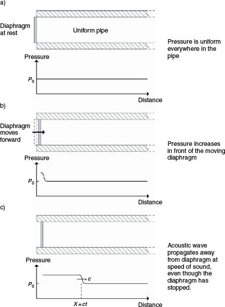
Figure 1.1 The generation and propagation of an acoustic wave in a uniform pipe

1.4.2 Mechanical and acoustic impedance

The description of sound propagation in Section 1.4.1 mentioned the motion of the air in response to local pressure differences. This localised motion is often described in terms of acoustic particle velocity, where the term ‘particle’ here refers to a small quantity of air that is assumed to move as a whole. Although we tend to think of a sound field as a distribution of pressure fluctuations, any sound field may be equally well described in terms of a distribution of particle velocity, and there is a relationship between the distribution of pressure in a sound field and the distribution of particle velocity. At a given frequency, the ratio of pressure to particle velocity at any point (and direction) in a sound field is known as acoustic impedance (strictly specific acoustic impedance), Z_a = p/u, and it is very important when considering the sound power radiated by a source. Acoustic impedance can be thought of as a quantity that expresses how difficult the air is to move. A low value of impedance tells us that the air moves easily in response to an applied pressure (low pressure, high velocity), and a high value of impedance tells us that it is hard to move (high pressure, low velocity). Mechanical impedance is directly equivalent to acoustic impedance, but with pressure replaced by force (pressure is force per unit area) and particle velocity replaced by velocity: Z_m = F/u.

With acoustic radiators, as well as electrical circuits and mechanical systems, there is a need to match impedances for good energy transfer. If a microphone needs to be connected to a 600 ohm input, then it will not sound as intended by its designers or exhibit its quoted sensitivity if connected to a 30 ohm or 10,000 ohm input. An amplifier which is optimised to function into a 4 ohm load will not produce its maximum power output capability into a load of 16 ohms. Loudspeakers are effectively ‘plugged into’ the air, so if the air load impedance does not match the electromechanical output impedance of the loudspeaker, the radiated power will be less than optimal. Impedance changes with frequency, so, for example, a resistor and capacitor in parallel have a frequency dependent impedance which is the combination of the purely resistive, frequency independent characteristic of the resistor, and the reactive, frequency dependent characteristic of the capacitor. This is the basis of electrical filter design.

Impedance (Z), whether it be electrical, mechanical or acoustic, can be divided into two components, resistance (R) and reactance (X). Reactive impedances represent systems which store input energy, but which later give it back, whereas resistive impedances represent systems which transfer energy away from the input, never to return. Figure 1.2 shows three mechanical systems which can be used to demonstrate the three different components of mechanical impedance and the way in which they relate to conventional loudspeakers. In Figure 1.2(a), the person applies a force to compress a spring. When the applied force is stopped, the spring returns to its original length and all of the (potential) energy applied to the spring is returned to the person as the spring pushes back. If the person pushes back and forth on the spring in an oscillatory manner, the energy flows from person to spring and back again in each half-cycle with an overall zero transfer of energy. A spring represents a purely reactive mechanical impedance. Figure 1.2(b) shows the person applying a force to a mass on a trolley. The force acts to accelerate the mass from rest, but when the force is stopped the mass tries to continue moving at a steady velocity. If the person then applies a force to slow the mass down, the (kinetic) energy possessed by the mass is returned as the mass pulls back on the person. Again, if the force is applied in an oscillatory manner, there is zero overall transfer of energy from the person to the mass. A mass also represents a purely reactive mechanical impedance, but with the opposite sign to that of a spring. (Note the different direction of the reactive force arrows in the figure.) Figure 1.2 c) shows the person pushing a block along a table. The applied force overcomes the friction between the block and the table and the block moves with a constant velocity. When the force is stopped the block also stops, and none of the energy supplied to the block is returned to the person. If the force is applied in an oscillatory manner in this case, the flow of energy is always from person to block, regardless of the direction of motion. All of the energy is ‘lost’ to friction as heat, and none is returned to the person. The friction block represents a resistive mechanical impedance which is the mechanism by which power can be transferred from one system to another (in this case, from the person to heat). There are acoustic counterparts to each of these mechanical components, for example, a small sealed cavity driven by a piston is an acoustic spring. The electrical counterparts will be further discussed in Section 1.6.

Figure 1.2 Three characteristic properties of a moving coil loudspeaker depicted as three components of its impedance. In electrical terms, these can be related to capacitance, inductance and resistance

1.4.3 Impedance in loudspeakers

In a cone loudspeaker, we have all of these forms of impedance present at the same time. The diaphragm radiates useful sound power through its motion via an acoustic radiation resistance. The mass of the voice coil and diaphragm, together with the stiffness of the suspension, produce a reactive impedance which merely serves to reduce the diaphragm motion. The reactive inductance of the voice coil reduces the current, and hence the applied force, at higher frequencies. And finally, the resistive frictional losses in the suspension and the electrical resistance of the voice coil simply waste power by turning it into heat.

1.5 The practical moving-coil cone loudspeaker

The majority of all loudspeakers are moving coil devices employing a cone-shaped radiating diaphragm, but the mechanisms of sound radiation from these devices are not as straightforward as they may initially seem to the casual onlooker. This type of loudspeaker is essentially a ‘volume velocity’ source. In other words it creates a pressure wave equivalent to injecting air from a point source at a rate of injection measured in cubic metres per second (or extracting the air on the rarefaction half cycle). However, unlike the piston shown in Figure 1.1, most cabinet-mounted cone loudspeakers, direct radiating into a room (i.e. not radiating via a horn), do not couple effectively with the air. Instead, the cone finds itself punching into thin air, with much of the potential load being lost as most of the air adjacent to it simply moves out of the way, then returns when the direction of the cone movement reverses. Efficiency is therefore often extremely low, with less than 1% of the energy being supplied to the voice coil resulting in the radiation of sound. The remaining energy either gets lost by friction in the moving system, or by being burned up as heat by the resistance of the voice coil, or even by being reflected back into the output stages of the power amplifier. To complicate matters, many of these things are frequency dependent, so, it is little wonder that many things must be considered and balanced before there is any chance of such a device having a flat frequency response.

As long as the circumference of the diaphragm remains small with respect to the wavelength, the radiation will be omnidirectional, but when the wavelength starts to become small compared to the circumference of the source, the radiation begins to beam directly ahead. [The wavelength, in metres, can be calculated simply by dividing the speed of sound in metres per second by the frequency in hertz.] This is a result of the interference field where the different parts of the diaphragm, radiating in phase, become significantly different in their path lengths to an off axis listening position. The cause is depicted in Figure 1.3, and the effect is shown in Figure 1.4. The ka values referred to in the latter figure are derived from the wave number k, which is simply 2π divided by the wavelength (λ) in metres, and a, which is the radius of the radiating surface. In practice we can think of ka as being the number of wavelengths around the circumference of the diaphragm: ka = 2πa/λ.

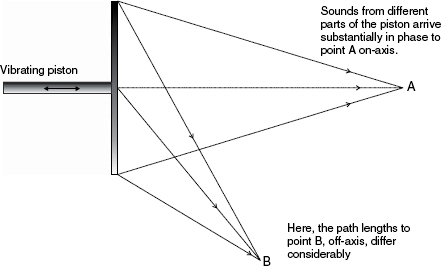
Figure 1.3 The cause of the off-axis interference effects that give rise to the directivity shown in Figure 1.4

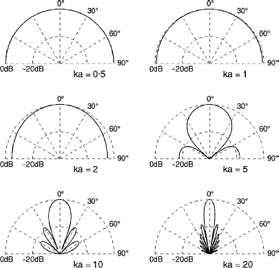
Figure 1.4 The directivity of a vibrating piston due to off-axis interference effects at different frequencies. Note the narrowing of the main lobe as the frequency increases

We would tend instinctively to think of the whole diaphragm as being the radiating surface, however, this is often not the case, and a large diaphragm driven at high frequencies will almost certainly not move uniformly. The outer parts would lag with respect to the movement of the central area, in which case the outer parts would radiate with a phase shift relative to the central area of the diaphragm. In fact they may even simply stay still, in which case they would not radiate at all. In either case the radiation may not correspond with the ka value taken from the physical measurements of the diaphragm.

Over the years, many ‘solutions’ have been tried in the search for perfect pistonic motion in a diaphragm, such as using ultra-rigid cone materials, or solid, conical ‘plugs’ as diaphragms, but internal losses and differential sound speeds within the materials have tended to confound all efforts. Remember, it was stated at the beginning of this chapter that air was not typical of all materials in terms of the speed with which sound propagates though it being equal for all frequencies. Many types of solid materials propagate high frequencies faster than low frequencies, a property known as phase dispersions, and exhibit sound speeds very different from that in air.

When the sound propagates from the voice coil through the material of the cone, in a radially outward direction, the different sound speeds may give rise to interference between the sound waves travelling to the edge of the cone and the forward radiation into the air by the pistonic action of the whole cone being driven by the voice coil. Resonances can also be set up within the cone itself, and one job of the cone surround is to absorb as much as possible of the waves propagating radially through the cone material, to prevent them from being reflected back and causing even more interference. Complex cone surrounds are often as much to do with suppressing these waves as with linearly suspending the cone itself.

1.5.1 The combined response

It was stated earlier that a loudspeaker was an electro-mechanico-acoustic transducer. Well, we have just looked at a few of the acoustic properties, but the electrical and mechanical aspects also present their own complications. The voice coil is a mixture of resistance and inductance, the latter being a form of frequency dependent reactance. The reactance, in ohms, of an inductor is given by 2πfL, where f is the frequency in hertz and L is the inductance in henries. An 8 ohm voice coil is only nominally 8 ohms, and approximates that value only over a limited band of frequencies. The inductive part of the impedance (impedance here being resistance plus reactance) rises with frequency, whereas any capacitive reactance effects decrease with frequency. The reactance(c) of a capacitor, in ohms, is given by 1/2πfc, so the frequency component, being in the denominator in this case, reduces the reactance as it rises. An overall impedance plot of a typical low frequency loudspeaker with respect to frequency is shown in Figure 1.5.

Fortunately, however, some effects counterbalance each other. Figure 1.6 shows how a flat frequency response can be achieved above the resonance frequency of a cone driver, mounted on a theoretical infinite baffle, where the roll-off in the diaphragm velocity compensates for its rising relationship with the pressure radiated to a point far away on the cone axis. However, at very close distances some rather more complex relationships manifest themselves. Academically speaking, this region is known as the near-field, but it should not be confused with the more colloquial ‘near-field’ that many recording personnel speak of. In fact, it is better to use the term ‘close-field’ for desk-top monitors, because the true near-fields are not good distances to listen within as the frequency balance can be strange in those regions.

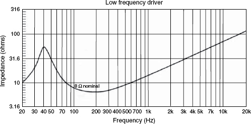
Figure 1.5 Magnitude of electrical impedance of a typical loudspeaker drive unit

Figure 1.6 How a flat frequency response results from a falling velocity and a rising radiated sound pressure

For people conversant with electrical circuit diagrams, equivalent circuits can be devised which represent the electrical, mechanical and acoustic properties of a loudspeaker as a single electric circuit. This type of representation is very common in traditional text books on electroacoustics. In these circuits, the mechanical and acoustic components such as springs and masses are replaced by their electrical equivalents. One way in which this can be realised is to replace mechanical forces (and acoustic pressures) with electrical currents, and mechanical velocities with electrical voltages. It follows then that mechanical springs are replaced by electrical inductors, masses are replaced by capacitors, and mechanical resistances are replaced by resistors. This arrangement is known as the mobility analogy, although it should be noted that a different, but equally valid, impedance analogy exists, where voltages replace forces and currents replace velocities. Each analogy has its strengths and weaknesses and may better suit different aspects of loudspeaker analysis. The equivalent mobility analogy circuit of a typical moving coil loudspeaker is shown in Figure 1.7. The transformers represent the coupling between the electrical and mechanical, and the mechanical and acoustical domains. This type of circuit is what an amplifier really ‘sees’ when terminated by a typical moving coil loudspeaker, which is a far cry from a resistive 8 ohm load.

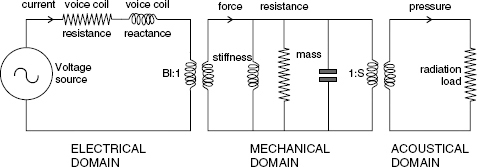
Figure 1.7 The equivalent electrical circuit of a moving coil loudspeaker drive unit (mobility analogy): Bl = the product of the magnetic flux density and the length of wire in the magnetic field – the force factor – T_m (tesla × metres): S = area of the cone

Getting a frequency-independent acoustic output from such a combination of components is no simple task. It can only be achieved by very careful balancing of the values of the components, and even then the perfect balance is usually only achievable over a limited bandwidth. It is apparent that any extra series resistance increase, or any parallel resistance decrease, will serve to reduce the power supplied to the load for any given input power, and so will reduce the efficiency of the system. What is more, with such a finely balanced system, any change to any component part(s) may require a counterbalancing change to many other component parts. As true perfection can never be achieved, there are an infinite number of close approximations which are possible, and this fact contributes to the diversity of loudspeaker designs that we have available in the marketplace.

1.6 Resistive and reactive loads

Before ending this introductory chapter, it may be worth looking a little more closely at the concepts of resistive and reactive loading. Figure 1.8 shows three potential-divider networks. If we consider a constant voltage source to be applied between terminals A and C we can consider what voltages occur between points B and C, and how much power will be dissipated in each component. In the case of the resistor-resistor network shown in Figure 1.8(a), the resistance of the two components R₁ and R₂ is equal. In a resistor, as the voltage is increased across its terminals the current will also increase in direct proportion, as given by Ohm's law, which may be written in the following ways:

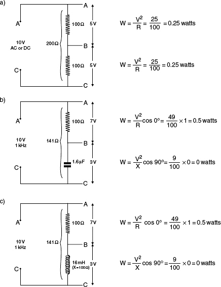
Figure 1.8 Three potential divider networks. W = watts, V = volts, R = resistance (ohms), X = reactance (ohms), Cos 0 degrees = 1, Cos 90 degrees = 0. In each case the total power dissipation is the same, at 0.5 watts, but it is only dissipated in the resistors. The inductors and capacitors merely store the energy then release it into the resistors. Note that a total of 0.5 watts is dissipated in each case

Where	I	=	current in amps
	V	=	voltage in volts
	R	=	resistance in ohms

The voltage and current are always in phase, so they will produce power, in watts (W), according to a simple multiplication:

Strictly speaking, this should be multiplied by the cosine of the phase angle, but as this is 0 degrees in resistive circuits, and the cosine of 0 degrees is 1, then a multiplication by one has no effect, so it is traditionally omitted. Whether the current is direct or alternating is also of no consequence in resistors, and the resistance remains the same irrespective of frequency.

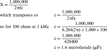
In the case of capacitors, there is a frequency dependent effect. Capacitors will not pass DC, because the impedance (reactance in this case) at 0 Hz is infinite, but as the frequency rises, the reactance lowers. Reactance (X), like impedance (Z) and resistance (R), is measured in ohms, but unlike resistance it is frequency dependent. In the case of capacitors, the reactance is inversely proportional to the frequency: as the frequency rises the reactance lowers. The formula for the reactance (X) of a capacitor is given by:

where	f	=	frequency in hertz
	c	=	capacitance in farads
	π	=	3.142

or,

where c is in microfarads

In capacitors, the current and voltage are not in phase, but are shifted by 90 degrees. In the case of Figure 1.8(b) an application of a DC voltage across A-C will initially see an uncharged capacitor behaving like a short circuit (zero ohms). A current will then flow through R and the plates of the capacitor will begin to charge. As the voltage rises across B-C, the current will reduce until, once the plates are fully charged, the voltage will rise to a maximum (as across A-C) and the current will reduce to zero. All conduction will then cease. Thus it can be seen how the current leads the voltage: the current flows first, then it falls as the voltage rises. The electrostatic charge is a voltage effect.

In the case of Figure 1.8(c) the effect is the reverse. Inductors work on an electromagnetic principle, which is a current effect. The formula for the reactance (X) of an inductor is given by:

Where:	f	=	frequency in hertz (Hz)
	L	=	inductance in henries (L)

In this case, the reactance is directly proportional to the frequency. As the frequency rises, so does the reactance, and the voltage leads the current. In the cases of both the capacitor and the inductor, the voltage and current are 90 degrees out of phase. Equation 1.4 showed the formula for calculating the power from the voltage and the current, and it was noted that for AC currents and voltages there should be a phase angle multiplier, cos (theta). The cosine of 90 degrees is zero, therefore whatever values of voltage and current exist in the circuit, the power dissipation (heating effect) in inductors and capacitors is always zero, (except for losses due to imperfections). This is wattless power, and is why AC power circuits are measured in VA (volt-amps) and not in watts. Electricity meters measure kVA because in heavily inductive loads, such as electrical motors and machinery, the kW value would be less, and the electricity company would not be charging for all the current and voltage that they were supplying.

In Figure 1.8(a), a 10 volt, 1 kHz voltage at terminals A-C would give rise to a voltage of 5 volts across B-C if R₂ was equal to R₁, at say 100 ohms each, and the resistors would heat up with the power dissipation. In the case of Figure 1.8(b), we could select a capacitor to have a reactance of 100 ohms at 1 kHz, but the circuit would not behave in the same way. The capacitor would be selected from the formula

However, despite the resistance and reactance in the circuit both being equal at 100 ohms, the total impedance (resistance plus reactance) would not be 200 ohms. The same current would flow through both components, but whereas the voltage across the resistor would be in phase with the current, the voltage across the capacitor would be 90 degrees out of phase with the current. We can draw a right-angled triangle, as in Figure 1.9, with one side representing the resistance and the other side, at 90 degrees, representing the reactance. The total impedance (Z) would be represented by the hypotenuse. From Pythagorus’ theorem, the square of the hypotenuse is equal to the sum of the squares of the other two sides. Therefore:

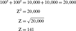
total impedance = 141 ohms

The resistor would dissipate power in the form of heat, but the capacitor would dissipate no power, and would not heat up. The inductive circuit in Figure 1.8(c) would behave similarly, except that the phase of the voltage across the inductor would be 90 degrees out with the voltage across the resistor in the opposite direction to the phase shift across the capacitor. The 90 degree differences in opposite directions leads to the 180 degree phase shift between capacitors and inductors, which gives rise to the resonance in tuned circuits. A capacitor and inductor in series are the electrical equivalent to the mass and the spring shown in Figure 1.10. Both are tuned circuits, and both work in the same way, by transferring energy backwards and forwards and dissipating very little of it. The mass takes in energy when one tries to move it, but releases it again when one tries to stop it – this is why the brakes get hot when a car stops. A spring takes in energy when it is stretched or compressed, but releases it when it is released. A mass, basically, ‘wants’ to stay free of accelerations and decelerations. A spring, basically, does not ‘want’ to change its length. The two together, given their different phase relationships, take in and release energy alternately, and so remain in oscillation until frictional losses eventually turn the energy into heat.

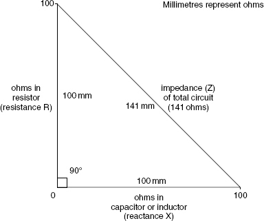
Figure 1.9 Phase angle vector triangle, using 1 mm to represent 1 ohm

At the risk of labouring the point (but it is really not well understood by most loudspeaker users) if we have a mass and a spring as shown in Figure 1.10(a) at equilibrium, the spring is ‘happy’ because it is at its equilibrium length given the forces acting upon it. The mass is also ‘happy’ because it is at rest; it is neither accelerating nor decelerating. If somebody then pulls down on the mass, and holds it there, the mass is still happy, but the spring is not, because it is stretched as in Figure 1.10(b). If the mass is released, the spring will act to overcome the inertia of the mass so that it can return to its equilibrium length. When the spring reaches its equilibrium length the mass is in motion, so the mass times velocity gives it momentum, which will carry it through the rest position of the spring, and will begin to compress it, as shown in Figure 1.10(c). The ‘unhappy’ spring therefore begins to slow the mass, so that it (the spring) can once again return to its ‘happy’ equilibrium position, but it overshoots once again, and the oscillation continues. This is a reactive system like a capacitor and inductor, and the only energy loss is due to its imperfection; which in the mechanical case is friction and air resistance, and in the electrical system is electrical resistance due to the less than perfect conductors – the coil of an inductor will always have a small resistance due to the wire.

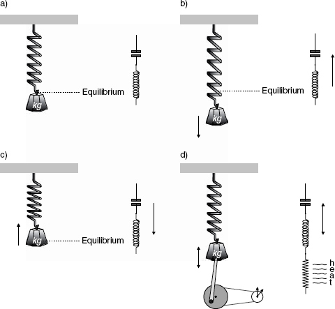
Figure 1.10 Masses, springs and resistances vis-à-vis inductors, capacitors and resistors

Now, if we add some resistance to the mechanical system, we can make it do some work, like moving the hands of a clock, as in Figure 1.10(d), but the work takes energy, so the oscillations will be reduced more rapidly – the oscillations will be damped. The electrical circuit equivalent would be to put a resistor in series with the inductor and the capacitor, so that the current flowing through the circuit will produce some heat, and damp the electrical oscillation.

When we load a loudspeaker diaphragm with a horn, the air in front of the loudspeaker cannot escape to the side of the diaphragm, and the stretching pressure due to the sideways component of the wave is restricted. The reactive conditions are therefore minimised, and the air load in the horn provides a substantially resistive load, with the particle velocity and pressure in phase, so more useful work can be done by the diaphragm, such as producing sound instead of just flapping backwards and forwards.

These concepts are relative to horns and direct radiators with their predominantly resistive and reactive loadings respectively. The resistive horn loading tends to be efficient because it gives rise to acoustic power being radiated. The largely reactive loading on a direct radiator gives rise to little power being radiated, just as little heat is produced in a capacitor or an inductor.

1.7 The bigger picture

This chapter has tried to set out the fundamental characteristics of sound radiation from moving coil loudspeakers, which represent 99% of all drive units manufactured, but up to now we have only been referring to single drive-units, which as we have previously discussed cannot be realistically expected to cover the full frequency range. Once we are forced to consider multi-driver systems with their obligatory crossover filters, the combined system can take on a further considerable degree of complexity. Many entire loudspeaker systems, some of great complexity, are made only from drivers using this motor technique. However, there are many other types of drive systems which will be discussed in the following chapter, and which we will need to look at in order to get a better appreciation of the characteristics which they can offer. Chapter 3 will then discuss the enclosures in which we must mount them, because the cabinets give rise to their own, extra complications as they affect the air loading on the diaphragms of open-framed drive units. Once we put the whole loudspeaker assemblies into rooms, as described in Chapter 7, a further set of complications arise. As all of these aspects of loudspeaker design and use compound each other, achieving a uniform response in all cases is not possible. For this reason, as perfection is not possible, much of this book will discuss the aspects of what we hear and what we may need to hear at various different stages of the music recording process; and, of course during the ultimate objective of domestic listening enjoyment. It will become apparent that it is all about compromise, but the optimum compromise points cannot be chosen without a thorough understanding of the overriding priorities at each stage of the process. A single driver is only a very small component part of a complex system that takes a musical signal from the amplifier to the ear.

References

1  Fahy, F., Walker, J., ‘Fundamentals of Noise and Vibration’, Chapter 5, Spon Press, London, UK, (1998)

2  Rice, C., Kellogg, E., ‘Notes on the Development of a New Type of Hornless Loudspeaker’, Transactions, American Institute of Electrical Engineers, Vol 44, pp 461–475, (1925)

3  Briggs, G., ‘Loudspeakers’ Fourth Edition, Wharfedale Wireless Works Ltd, Bradford, England (1955) – Reprinted by Audio Amateur Publications Inc, Peterborough, NH, USA (1990)

Bibliography

1  Borwick, J., ‘Loudspeaker and Headphone Handbook’, Third Edition, Focal Press, Oxford, UK (2001)

2  Colloms, M., ‘High Performance Loudspeakers’, 6^th Edition, John Wiley and Sons, Chichester, UK (2005)

3  Eargle, J. M., ‘Loudspeaker Handbook’, Chapman and Hall, New York, USA (1997)

4  Briggs, G. A., ‘Loudspeakers’, Fifth Edition, Rank Wharfedale Ltd, Bradford, UK (1958) – Reprinted until 1972

5  Jordan, E., ‘Loudspeakers’, Focal Press, Oxford, UK (1963)

6  Borwick, J., ‘Loudspeaker and Headphone Handbook’, Second Edition, Focal Press, Oxford, UK (1994) (significantly different in content from the aforementioned Third Edition.)