Chapter 9

Subjective and objective assessment

9.1 The general situation

The human hearing system is quite extraordinarily sensitive and complex. It has a frequency range of around eleven octaves if one considers physical sensation as part of the process, and a dynamic range such that the lowest audible sounds have power levels of only 10−12 compared to the loudest sounds before the threshold of pain in the ears. That is a power ratio of one million, million times (one trillion in American English). At the lowest detectable sound pressure levels, the lateral movement of the ear drum, (or tympanic membrane) is less than the diameter of a hydrogen molecule, and if the average ear were only 9 or 10 decibels more sensitive, we would experience a permanent hissing sound due to the detection of the Brownian (random) motion of the air molecules. The signal processing of sounds by the brain is also a remarkably refined process. It is thus little wonder that when we reproduce music via the relatively crude devices described in Chapter 2 we are rarely fooled into believing that we are listening to the real instruments.

Nevertheless, back in 1990 David Moulton made the case that loudspeaker reproduction has now reached a stage where, at least with many musical styles, it should be recognised as something in its own right¹. Music is now being created on loudspeakers for reproduction by loudspeakers, and much of this music exists in no other form. For many musical creations there was never, at any place or any time, a complete performance of the music as recorded. The late Richard Heyser, the ‘father’ of the ‘Time Delay Spectrometry’ measuring system said that in order to really enjoy stereo reproduction, one has to willingly suspend one's belief in reality. We must therefore ask ourselves if we are really trying to reproduce a sense of ‘being there’ at the original performance, or is there a ‘being there’ at the reproduction, which may be far more exciting than any live performance could ever be, because it must be accepted that some reproducible music simply could never be performed live. Are we now, as David Moulton asked, so accustomed to reproduction via loudspeakers that the loudspeakers, themselves, have become the greatest musical instrument of our time?

We seem now to have two separate outlooks on loudspeakers for music reproduction: ‘the closest approach to the original sound’, as the Acoustical Manufacturing Company put in their advertisements in the 1940s, or ‘the best sound that we can possibly get’, with ‘best’ being highly arbitrary. Nevertheless, it seems that from whichever viewpoint the subject is approached, the general requirements tend to be rather similar: wide bandwidth, low distortion, adequate sound pressure level, fast transient response, low colouration, and so forth. The degrees to which the levels of discrepancies of each aspect of the response are acceptable may vary with the musical styles and the listeners’ preferences, but John Watkinson's point of view, that the only criterion we have for the accuracy of a loudspeaker system is the sensitivity of the human hearing system², seems to be quite valid. He went on to say that if a reproduction system is more accurate than the human hearing system's error detection threshold, then it needs no further improvement. Nonetheless, that is a difficult goal to achieve when we consider what was discussed in the opening paragraph of this chapter. As shown in Chapter 7, the human hearing system is dealing with wavelengths from as great as around 20 metres to as small as about 1.5 centimetres, a ratio of over 1000 to 1. By contrast, the eye has to deal with almost a one octave range of visible light spectrum, a wavelength ratio of less than 2:1.

Strictly speaking, we would only need one test for a perfect loudspeaker: its ability to perfectly reproduce a delta function supplied electrically to its input terminals. A delta function, otherwise known as a Dirac function, or impulse, contains all frequencies in a very fixed phase relationship, and its waveform is shown in Figure 9.1. Unfortunately, no mechanical system can start and stop instantaneously, so this waveform can never be perfectly reproduced. A delta function reproduced by a good loudspeaker is shown in Figure 9.2, and the degree of reproduction error is patently obvious. Unfortunately, we cannot glean all the information that we need from a visual inspection of the delta function response, so we tend to use a series of individual measurements which highlight particular aspects of a response. Some of them show behaviour in the frequency domain, whilst others show behaviour in the time domain. From them we can build up a picture of how a loudspeaker is responding to its electrical input stimulus, and shortcomings in the response can be assessed.

9.2 Test signals and analysis

The most well known aspect of any loudspeaker performance is the magnitude of the frequency response, which appears in just about every advertising leaflet for loudspeakers. In fact, the full frequency response also needs to show the associated phase response, and from the full response every linear aspect of a loudspeaker performance can be derived. A system may be said to be linear if the output contains no frequencies which do not exist in the input signal. A roll-off, or any other deviation from flatness in the frequency response, can be called a linear distortion. A system is said to be non-linear when frequencies exist in the output which were not present in the input signal. For example, if a pure sine wave were to be fed to the input terminals of a loudspeaker, and the measured output showed small amounts of response at twice the frequency and three times the frequency, then those additional frequencies would be the second and third harmonics of the input frequency, and the loudspeaker would thus be generating non-linear distortion; in this case harmonic distortion. If the loudspeaker is fed with multiple input frequencies, anywhere from two upwards, then a non-linear system would also produce sum and different tones. In such a case, if the input were to be fed with 1 kHz and 4 kHz, for example, outputs would be noticed also at 1 + 4 kHz, or 5 kHz, and 1 − 4 kHz, or 3 kHz. The products can also further create their own sum and difference tones, and also inter-react with the original tones, producing frequencies such as 3 kHz + 4 kHz (7 kHz), 5 kHz + 1 kHz (6 kHz) and so forth. Whilst harmonic distortions in themselves are not necessarily unpleasant, because all musical sounds are rich in harmonics, the sum and difference products, known as intermodulation distortion, can be grossly offensive to the ear.

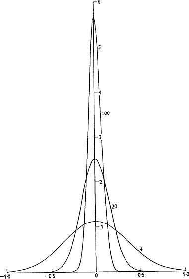
Figure 9.1 Evolution of the Dirac delta function (reproduced from Lighthill, 1964)

In a delta-function one can imagine the energy in a unidirectional signal being gradually narrowed, and each time that it narrows the amplitude increases until, in extremis, it becomes a pulse of infinite height and infinitesimal width

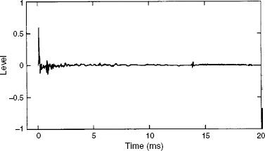
Figure 9.2 Loudspeaker reproduction of an impulse

The Dirac delta-function when reproduced by a loudspeaker inevitably becomes bi-directional and smeared in time, due to the imperfect reproduction

They may or may not coincide with musical harmonics, and they tend to build up into a noise-like signal which accompanies the music. Briggs, in his book Sound Reproduction, published in the 1950s, summed up the situation beautifully in a short quotation from Milton with which he introduced his chapter on intermodulation distortion – “. . . dire was the noise of conflict.”³ In fact, Gilbert Briggs was so disturbed about the problem of intermodulation distortion that he invited a more knowledgeable specialist, one N.C. Crowhurst, to write the chapter in the Third Edition of the book. In the Second Edition, published in 1950, Briggs had quoted Shakespeare in the chapter on intermodulation which he had written himself (Briggs, that is; not Shakespeare!):

Find out the cause of this effect;

Or rather say, the cause of this defect,

For this effect defective comes by cause.

Hamlet, Act II, Scene 2.

Over 50 years later, intermodulation distortion is still a significant problem, and we still have no simple way to measure it in an easily interpretable way which intuitively relates to all its audible implications.

Time domain representations of performance are less frequently published, and even less widely understood by loudspeaker users. Nevertheless, they are essential aspects of the analysis of loudspeakers because the phase response, which in concert with the amplitude response is sufficient to define all linear aspects of performance, is very non-intuitive. Phase is very abstract; it is a relationship between things, and cannot exist alone. Time domain representations include waveform responses, such as Dirac (delta) and Heaviside function responses (impulse and step-function responses), acoustic source plots which show group delay against frequency, and cepstrum plots, which are useful for finding reflexion and diffraction problems in otherwise complex signals. It is perhaps useful, now, to look at all of these representations and their implications step by step.

9.2.1 Frequency response plots

Figure 9.3 shows a frequency response plot of the axial response of a loudspeaker, derived from a pink noise signal and a dual channel analyser which compared the direct electrical input with the acoustic output, in an anechoic chamber via a measuring microphone. Both the amplitude and phase responses are shown, and it can be seen how there can be no deviation from a straight line in either curve without a corresponding deviation in the other. This is the characteristic of a minimum phase response as discussed in Chapter 7.

Figure 7.19 shows clearly how the amplitude response plots change as equalisation is introduced into a system. Almost everybody reading this book will understand the significance of the amplitude part of the plot, and how ideally, for perfect reproduction the line should be as flat as possible and as wide as possible. From an objective point of view the magnitude plot tells the engineers much about the uniformity, or otherwise, of the pressure amplitude response with respect to different frequencies, and consequently, if those design aims have been achieved.

Subjectively, it has long been considered that the magnitude of the pressure amplitude response (the frequency response in everyday language) is the most significant measure of a loudspeaker's performance, and yet no loudspeakers are truly flat. Smooth deviations from flatness are generally acceptable, and are easily grown accustomed to by listeners who are familiar with the loudspeakers. Many mastering engineers consider extreme flatness to be nice if it can be achieved without other compromises being made, but not essential, because a smooth frequency response deviation is a linear distortion which can be compensated for both mentally and electrically without having to pay the penalty of side effects. On the other hand, abrupt changes or irregularities in the frequency response are definitely undesirable. They not only introduce colouration which will only affect music with dominant signal content in the region of the irregularity, but they almost always imply that something else is wrong in the system, and that the abrupt changes are only side-effects of whatever that something else may be. The physics of loudspeaker design really does not permit abrupt changes in frequency response without other consequences, so smoothness is a very desirable characteristic of a curve, perhaps more so than general flatness with an abrupt change somewhere. Abrupt changes are usually accompanied by time response anomalies.

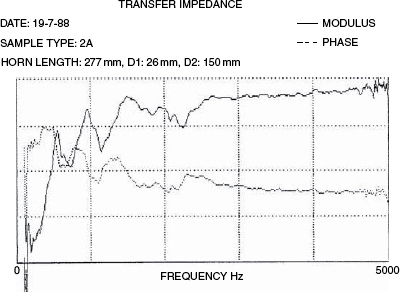
Figure 9.3 A full frequency response

The frequency response of a mid-range horn loudspeaker

The vertical divisions represent 10 dB in amplitude or radians in phase (360 degrees/2 = about 57 degrees). It can be seen how every change in the upper, pressure amplitude plot is accompanied by a corresponding deviation in the lower, phase plot

Figure 9.4 shows a series of off-axis plots, both in the vertical and horizontal planes. Their significance is twofold. Firstly, any persons listening off-axis (that is, away from the line which is typically perpendicular to the centre of the face of the loudspeaker cabinet), will hear a response which is characterised by the respective plots in the horizontal and vertical directions. [Note that in a multi-way loudspeaker system it can be very difficult to determine exactly where on the face of the cabinet is the exact acoustic centre of propagation.] The acoustic centre of the loudspeaker shown in Figure 8.6(a) is rather obvious, but the acoustic centre of the loudspeaker shown in Figure 8.6(c) is not obvious at all. The second significance of off-axis frequency responses is that any reflexions which return to the listening position from off-axis radiations will be affected not only by the frequency response of the reflective surface, which for a plastered brick wall would be acceptably flat, but also by the frequency balance radiated in that direction from the loudspeaker. Many, large, multi-way monitor systems do exhibit poor off-axis responses, a price sometimes paid to allow for other design benefits, which is one reason why so many professional control rooms have rather absorbent side-walls that will not return reflexions to the listening position, or geometry that tends to direct this energy into absorbers after the first bounce.

Until now we have been looking at plots of anechoic responses, but once the room response becomes involved in the proceedings, the loudspeakers-only responses tend to get corrupted. Figure 9.5 shows the response of a loudspeaker in an anechoic chamber, and Figure 9.6 shows the response of the same loudspeaker placed on top of a mixing console in a typical small control room. The changes can be seen to be gross, but a measuring microphone is not a pair of ears and a brain. The ability of the ear to know when it is still receiving a smooth direct sound, despite all the chaos surrounding it, is something quite impressive. Moreover, human beings live and work in reflective environments, so if the response corruption is not excessive the irregularities are accepted as what they are – room effects. However, if the room reverberation or response decay time becomes significant, it can mask low-level detail in the sound, so the room decay time is an important factor where detailed monitoring is required. The acceptability or otherwise of room effects on loudspeaker responses may depend on the principal reason for listening, such as to the recording quality, or to the performance.

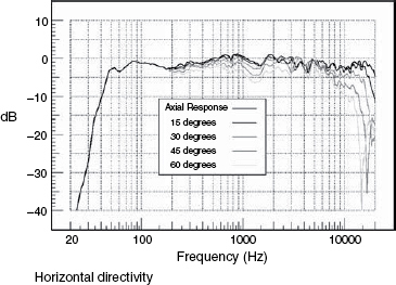
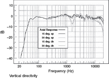
Figure 9.4 Horizontal and vertical directivity plots, showing the responses on-axis and at various angles off-axis

The phase of the frequency response is something which is more useful in engineering processes rather than as something that relates to clearly audible effects, except to say that gross phase errors will be discernible as time response effects.

9.2.2 Waterfall plots

A good general grasp of the performance of loudspeakers can be made from a visual assessment of their waterfall plots. These show a three axis representation of time against frequency against level, as shown in Figure 9.7. In effect, a waterfall plot is a series of pressure amplitude plots taken a few milliseconds apart and displayed by superimposition by computer after the input stimulus has been stopped. An ideal loudspeaker system, which could reproduce an accurate delta function, would show only the top line of the plot – the zero milliseconds line – because the decay would be instantaneous. As explained earlier though, no mechanical system can start and stop instantaneously, and the waterfall plots show how the decay takes place, frequency by frequency. A large selection of waterfall plots are shown in Figure 11.1 which are very informative. They show, without any shadow of a doubt, why virtually all loudspeaker systems sound different to one another: none of the responses decay in the same way.

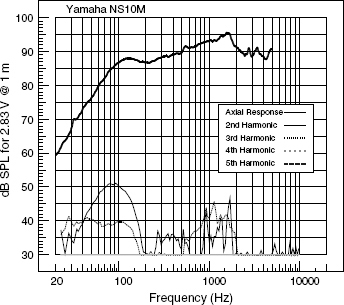
Figure 9.5 Anechoic measurement of frequency response

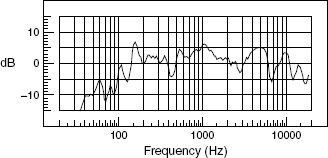
Figure 9.6 Console-top measurement of frequency response

The same loudspeaker as measured in Figure 9.5, but on top of a mixing console in a typical home-studio control room

Figure 9.7 A waterfall plot

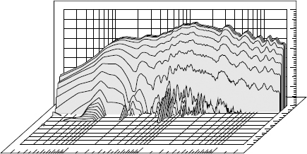
The cascading lines are the frequency (pressure) responses at 2 millisecond intervals after the cessation of the input stimulus (simulated) at time = 0 milliseconds. Various resonances can be seen continuing to ring until about 40 milliseconds

Subjectively, a long decay tail sounds exactly like what it is; resonance. Figure 9.8 shows the waterfall plots of two different loudspeakers of more or less the same size, a) being a sealed box and b) a reflex enclosure. The box concepts are dealt with in Chapter 3, and the implications are dealt with in Chapter 11, but the general tendency is for the loudspeaker with the faster decays to sound tighter in the bass; the longer decays sound rounder. Balances between bass guitars and bass drums tend to be more reliable and compatible with a range of other loudspeakers when mixed on faster decaying loudspeakers, because the resonances of the individual instruments are heard in a more realistic proportion with each other. Resonant loudspeakers will add their own characteristics to the sound, so it becomes difficult to judge exactly what part of the bass sound is due to the instruments alone, and which part is due to the loudspeakers. Relatively few top mastering engineers use reflex cabinets, and those who do use them tend to use relatively large cabinets with resonances very low down in the audible frequency range. It is believed by the authors that the long-lived and widespread use of the Aurotone 5C and Yamaha NS10 loudspeakers for rock music mixing was largely because of their rapid decays which were uniform with frequency. Even though their frequency responses in anechoic chambers were far from flat, they tended to flatten in the bass region when placed on top of mixing consoles due to the reduction in the radiating angle. Nevertheless, they were still rather bass light, but the accurate time response meant that the relative levels of bass instruments were not confused by resonances, so if the mix was deemed to be bass heavy on larger loudspeakers, it was a relatively simple matter to equalise the mix with a reduction of bass frequencies and still maintain the instrumental balances. This process is often not possible when the balance between the instruments has been confused by loudspeaker resonances. This is especially problematical when the resonant frequencies of the loudspeaker reflex port timing is above the 41 Hz fundamental frequency of the lowest note on a conventional 4-string bass guitar or double bass (the E-string).

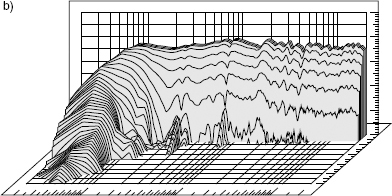
Figure 9.8 Waterfall plots of two loudspeakers. a) A small sealed-box loudspeaker with a relatively rapid delay. b) A small reflex loudspeaker with a considerably longer decay at low frequencies than at mid and high frequencies

Whether such instruments are recorded flat, or stylised by the use of equalisation and signal processing, the final sound must be judged to be suitable for reproduction via a wide range of loudspeakers. This is clearly a difficult task with the situation that exists. The responses shown in Figure 11.1 all represent loudspeakers designed for professional music recording and all were measured in the same anechoic chamber. The situation in domestic reproduction rooms and with non-professional loudspeakers is obviously more diverse. Whilst research has been done both by JBL and Genelec on finding the mean frequency response of a wide range of listening conditions, no such work seems to have been carried out to find the mean, most representative waterfall plot. It transpires that the mean frequency response (or at least the pressure response) is substantially flat, and many critical listeners also consider that loudspeaker decay times should also be uniform with frequency. Mastering engineers certainly seem to choose predominantly low decay-time loudspeakers – a choice which they have mostly made by ear – as they have found them to aid in the making of more consistent decisions, but the lack of any industry-wide guidelines on response decays is a great pity.

9.2.3 Harmonic distortion

Harmonic distortion plots cannot be generated from noise signals nor complex waveforms. The only practical method of producing a plot such as the one shown in Figure 9.9 is to send to the loudspeaker a sine wave tone which continuously sweeps up in frequency, covering the entire audible frequency range, and use a set of tracking filters which are spaced at one, two, three and four octaves above the principal tone. The outputs of these filters are the second, third, fourth and fifth harmonics of the input tone, and their relative levels can be given in percentages or decibels, which are compared below:

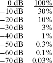
Hence, for example, in a loudspeaker which produces 0.3% of harmonic distortion, the distortion products would be 50 dB below the main signal. Another method, perhaps more commonly used, it to measure the level of a single tone, repeated at several different frequencies, and then to measure what remains each time when the frequency of the drive tone is filtered out of the response. This yields a ‘total harmonic distortion plus noise’ or THD + N figure for each single frequency that is measured, but THD + N has consistently failed to relate well, subjectively, to the perceived sound from loudspeakers. Below 50 Hz it seems to be very doubtful that second and third harmonic distortion levels as high as 5% are audible, and it seems questionably whether levels as low as 0.25% are audible at any frequency. The ‘maximum operating level’ for magnetic flux on analogue tape recorders was set for many years around the 3% distortion level, and some really beautiful sounding recordings were made on those machines. Furthermore, despite the fact that electronic systems, such as amplifiers, with the above levels of distortion could not even be considered for high fidelity use, they may, in some circumstances, make tonally rich sounding guitar amplifiers; so they may not be accurate, but they are not necessarily unpleasant sounding. There is also an enormous range of microphone preamplifiers on the market, all sold on the basis of their characteristic sounds, which effectively means their characteristic distortions. These distortions are considered desirable by many people during the recording process, although for monitoring purposes it is obviously undesirable to colour the sound or the concept of monitoring the recording would not be valid. Nonetheless, and again as mentioned in Chapter 6, such distortions are also considered to be desirable for musical instrument amplification, so we therefore need to face the problem of deciding what level of harmonic distortion is accepted as ‘non-intrusive’ for each piece of equipment in turn.

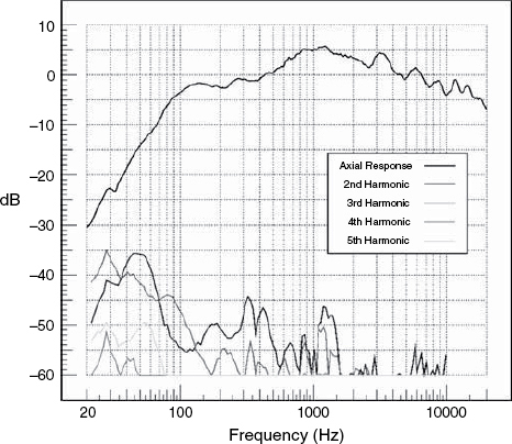
Figure 9.9 On-axis pressure amplitude and harmonic distortion

The problem with harmonic distortion as a quality measure in itself is that harmonics of a low order (2^nd, 3^rd, 4^th can actually be quite pleasant sounding, and not unmusical at all. All instruments produce large quantities of harmonics, sometimes even more than their fundamental tones, so the question was often asked as to how the ear could detect 0.2% of harmonic distortion from an amplifier reproducing an instrument whose tone was itself perhaps 80% or more of harmonics. The answer must lie in the differences in the mechanisms which produce the harmonics, and in what other ways those mechanisms manifest themselves.

A musical instrument produces harmonics from the break-up of its parts into separately resonating sections, which vibrate independently whilst they also vibrate as part of the whole. Figure 9.10 shows a representation of a string breaking into second, third, and fourth harmonic modes, and Figure 9.11 shows the vibrational patterns of a metal plate. Note the perfectly symmetrical behaviour. A harmonic analysis of the sound would be likely to show only frequencies which were harmonically related to the fundamental resonance.

When an amplifier produces harmonics, the mechanisms involved are totally different. Harmonics are produced as a result of the transfer function of the amplifier being non-linear, as shown in Figure 9.12, and by other means which are totally alien to natural vibrations, such as the crossover distortion mentioned in Chapter 6. Loudspeakers, also, behave entirely differently to either musical instruments, strings or plates because, at least for sound reproduction purposes, they are usually designed not to break up into separately moving sections, and they are unlike amplifiers because their moving parts have mass, and hence momentum when in motion. They also have non-linear stiffness in their suspension systems, and, amongst other things, they may have non-linear Bl products, where the drive force is not uniform because of the inconsistent relationship between the static magnetic field (B) and the length of coil (l) when being driven by the voice coil.

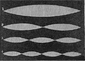
Figure 9.10 Vibrational modes in strings

Representation of a string vibrating, and showing how it can break up into multiple segments at harmonic intervals in response to stimuli at those frequencies

In fact, harmonic distortion is not a good measure of such subjective subtleties. Some loudspeakers can have 10 dB of difference in harmonic distortion levels yet they may sound very similar, or vice versa. During listening tests carried out by the authors in 1989⁴, in an attempt to group according to sonic similarity a selection of twenty mid-range drive units, harmonic distortion performance failed to show any relationship to the pattern of similarity groupings. The fact is that harmonic distortion is really the benign face of non-linear distortion, it is usually the intermodulation distortion which really offends the ear.

9.2.4 Intermodulation distortion

This subject has been investigated in depth by Czerwinski, Voishvillo and their co-investigators who have tried to make representations of analyses which relate measured intermodulation products with sonic perceptions^5.6. The problem with measuring these distortions is that they are so dependent upon circumstances that it has always been difficult to define them. Intermodulation distortion can change dramatically with level, with the frequency range of the music, with the crest factor of the music (the peak to average relationship) and with many other parameters. Generally, the more complex the musical signal, the more offensive is the intermodulation, as every frequency interacts with every other frequency and with the products of the intermodulation, which in turn intermodulate with themselves. For this reason, a loudspeaker system may sound totally acceptable on relatively simple musical signals, but may sound rather unpleasant with an orchestral crescendo or a heavy concentration of guitars. At the same time, it may well be the case that the perception of the purely harmonic distortion, even up to the higher harmonics, if the intermodulation distortion could be separated out, could be totally inoffensive. However, the harmonic and intermodulation products cannot be separated, because they are products of the same non-linear processes. Nevertheless, it is unfortunately misleading that the harmonic distortion, which can easily be measured, should so frequently get blamed for the undesirable sounds which are really a result of the intermodulation distortion, which cannot be so easily quantified. As no simple relationship exists between harmonic and intermodulation distortions, neither one can be extrapolated from the other.

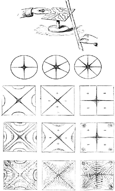
Figure 9.11 Vibrations in plates

An insight into diaphragm break-up. Nineteenth century experiments on vibrations in metal plates [From ‘On Sound’ by John Tyndall, Longmans Green & Co, London, (1895). Reprinted by Dover Press – highly recommended reading, and still in print]

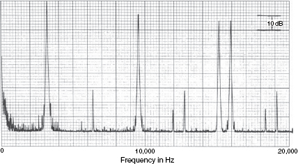
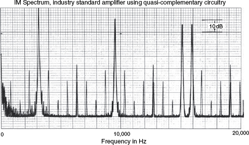
Figure 9.12 Non-linear transfer functions

The two transfer functions show very significant differences in intermodulation distortion in two amplifiers whose harmonic distortion figures are very similar to each other. The four highest peaks are the four frequencies of the drive signal. All the other spikes are distortion products of intermodulation

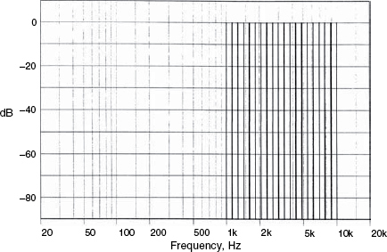
Figure 9.13 Spectrum of a 20-component logarithmic multi-tone signal

Figure 9.12 showed the greatly different levels of intermodulation and harmonic products of two amplifiers whose harmonic distortion products, alone, were measured to be very similar. Traditionally, intermodulation has been measured by pairs of tones, say 1 kHz and 5 kHz, but the results have never been particularly representative of any sonic characteristics of the systems under test. The tests shown in Figure 9.12 used four input tones, however, multi-tone signals using ten or twenty frequencies, specially chosen give rise to the widest spread of intermodulation products, can give a visual display of results which intuitively relate much better to what is heard. A twenty tone spectrum is shown in Figure 9.13, and its corresponding waveform is shown in Figure 9.14, which looks quite typical of a musical signal. In fact, statistically, it is also very representative of a real musical signal⁷. The response of a bass driver to a ten tone signal is shown in Figure 9.15⁷. The reason why intermodulation distortion is so audibly offensive can clearly be seen from this graphical presentation. Bear in mind that a distortion-free system would exhibit only the ten vertical lines of the stimulus signal, similar to the twenty, clean lines shown in Figure 9.13. The mass of sum and difference tones shown in Figure 9.15 are like a noise signal which changes dynamically and spectrally according to the stimulus. On a music signal it would be heard as a loss of transparency and openness in the sound, and a loss of low level detail. If the density of intermodulation products from only ten sine-wave tones is as high as shown in Figure 9.15, then it is easy to appreciate that a complex musical signal would produce an underlying, signal-related hash that could take the sweetness out of the music and mask room-sounds.

The fact that intermodulation distortion is the real enemy of both musicality and fidelity has been known since the very early days of loudspeakers⁸, but it is still so hard to quantify it in any meaningful way simply because it is dependent upon so many dynamic factors, and its subjective offensiveness is signal dependent to a much greater degree than is the case for harmonic distortion. The fact that the two types of distortion share the same origins is easily demonstrated by the use of two tones, one fixed in frequency and the other variable. If the two tones are different, the spectral lines on a frequency analysis would show the harmonics, plus the sum and difference tones. If the variable frequency source were to be swept to the same frequency as the fixed tone, the pattern of modulation products would change until with the two tones at the same frequency, only the harmonics would be evident. However, where intermodulation is concerned the products are dependent upon so many factors that no truly meaningful figure of ‘merit’ has been devised to unequivocally define intermodulation distortion performance. To quote from Czerwinski et al, “High-order nonlinearity is very sensitive to the level of the input signal. An increase in input signal which produces a negligible effect on low-order [harmonic] products can wake up the ‘evil forces’ of nonlinearity, releasing an unfathomable number of high-order intermodulation product ‘piranhas’ to tear the flesh of the reproduced sound to pieces”⁶.

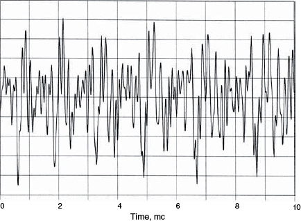
Figure 9.14 Waveform of a 20-component logarithmic multi-tone signal

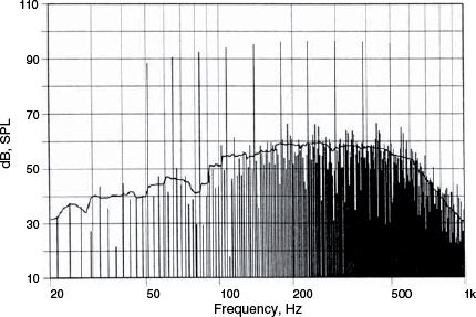
Figure 9.15 Sound pressure reaction of a loudspeaker (long coil, short gap) to multi-tone stimulus. The peak level of the input signal corresponds to X max = 4 mm. The solid curve shows the level of distortion products averaged in a one-third-octave-wide rectangular sweeping window

It has puzzled many people for many years why relatively low levels of high-order harmonic distortion – 5^th,6^th,7^th etc – have been associated with poor sound quality. The principal explanation has been that the higher harmonics are not musically related to the signal, but the very low levels of these distortions have not corroborated this idea when they have been added artificially to sine waves, where they have tended to be inaudible at levels which prove to be offensive on music. Czerwinski et al offer the explanation that the low levels of high-order harmonics are, in fact, just tips of high-order intermodulation distortion ‘icebergs’. It obviously does not bode well to be metaphorically sailing amongst icebergs in a sea full of piranhas! But that has been the reality of intermodulation distortion – a largely hidden, unquantifiable, yet dangerous enemy.

Distortion mechanisms which give rise to similar levels of harmonic distortion may yield greatly differing levels of intermodulation distortion, and this fact is surely at the root of the long acknowledged lack of any robust correlation between harmonic distortion measurements and subjective audio quality. Having said that, it is obvious that a loudspeaker producing 75% of total harmonic distortion (THD) at 1 kHz would not be considered to be high fidelity, but once we get into the low single figures at low frequencies, or below 0.5% at higher frequencies, then a loudspeaker with 10 dB less THD than another may well not guarantee that it would sound more musically accurate, even when their linear parameters were relatively similar. On the other hand, multi-tone intermodulation distortion presentations have begun to reveal good correlation between pure-sounding loudspeakers and clean-looking displays.

9.2.5 Delta-functions and step-functions

A delta-function is shown in Figure 9.16. It is a unidirectional impulse containing all frequencies, and of infinitesimal duration. The response to a delta function defines the full frequency response of any linear system. Mathematically speaking, the delta function is the derivative of the Heaviside function, also known as the step-function. The main problem with using a delta function (also known as a Dirac function, or impulse) in acoustic measurements is that it has very little low frequency content; having a spectrum rising by 3 dB per octave, like white noise. This results in a tendency towards poor signal to noise ratios at low frequencies, where air conditioning noise, ventilation noise and traffic rumble can prejudice the low frequency response accuracy of the acoustic measurement. The step-function (or Heaviside function), shown in Figure 9.17, contains much more low frequency energy. The fact that by processes of either integration or differentiation, either one can be transformed into the other makes the step-function a better option for acoustic measurements, even if it is the impulse response that is ultimately required. Numerous step-function responses are shown in Chapters 10 and 11.

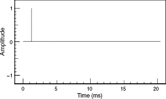
Figure 9.16 A Dirac delta-function, or impulse

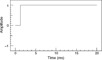
Figure 9.17 A Heaviside step-function

A simple circuit for a rudimentary step-function generator is shown in Figure 9.18. If this signal is applied 15 or 20 times to the input of an amplifier (sufficient to allow for an averaging process to disregard extraneous noises) with about 5 seconds each of ‘on’ and ‘off’ time, then by means of the FFT processing of a dual channel recording of the direct electrical output of the box and the loudspeaker output via a measuring microphone, the full frequency response of the transfer function of the system can be obtained. The pressure amplitude response, phase response, waterfall plots, acoustic source plots, cepstrum plots, impulse response and waveform response can all be derived from the step-function. Listening to the DC ‘thuds’ can also be quite revealing. A highly damped loudspeaker in an absorbent room will produce a very ‘tight’ impact. In many small control rooms, using small, reflex loudspeakers, the step function tends to sound like an ‘ideal’ bass drum – round and warm, yet solid. This exposes a dangerous situation for making decisions about bass drum/bass guitar/bass synthesiser sounds, because it suggests that much of the perceived sound is likely to be that of the loudspeaker and/or room, and that the ‘great’ sound is not on the recording. To get a better idea of what the step function really sounds like, it can be listened to on a pair of good quality headphones if a reference in anechoic conditions and via fast loudspeakers is not available.

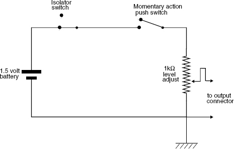
Figure 9.18 A step-function generator

This circuit will emulate quite well the waveform shown in Figure 9.17. For low impedance loads, such as direct connection to loudspeaker drivers, the potentiometer should be set to maximum. A good quality potentiometer should be used

The step function, used in this way, will also expose resonances from things such as open ended cable tubes in the control room, tubular steel mixing console frames, fire extinguishers, furniture resonances, window pane resonances and many other problems that ideally should not be in a critical listening environment. Figure 9.19 shows the response of a control room with open cable tubes in the floor. Although not obviously audible on a pink noise signal, the step source rendered their presence plainly audible to anybody in the room.

If a battery is used as a step source by coupling it and decoupling it directly to a passive loudspeaker system the effects will not be symmetrical, because during the ‘on’ phase, the battery will be connected across the loudspeaker terminals, and its low internal resistance will damp the loudspeaker resonance. On the other hand, when the battery is disconnected, the loudspeaker input terminals will be left open circuit, so the voice coil(s) of the low frequency driver(s) will be left unterminated and free to resonate. The sound of the on and off cycles may therefore sound, and measure, quite different. However, when the signal is supplied to the loudspeaker via a power amplifier, the low impedance of the output is permanently connected across the loudspeaker terminals, so the positive and negative signals should be much more similar. Bear in mind though that if a 11/₂ volt battery is used as a step source and connected to the input of a power amplifier for loudspeaker testing purposes, the amplifier should have a flat response down to DC, or the amplifier's roll-off would affect the loudspeaker's true low frequency response.

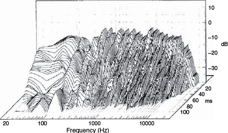
Figure 9.19 Cable tube resonances exposed by a switch box as described in Figure 9.18.

Resonances are clearly visible at about 70 Hz and 110 Hz due to open cable tubes in the control room floor. The resonances were clearly audible on step-function excitation

It should also be borne in mind that the human ear does not always hear the positive and negative pulses in the same way due to its own polarity asymmetry. For this reason a positive-going output from a mixing console or other music source should produce a forward (towards the listener) movement of the loudspeakers diaphragm(s). Although the effect is subtle, if this ‘absolute phase’ connection is not respected it can give rise to altered perception of the music.

And beware! Not all loudspeakers or drive units or amplifiers give a positive-going output from a positive-going input at their red terminals or signal ‘hot’ input connectors. Many JBL loudspeakers still follow an older standard where the application of a positive voltage to the red terminal causes a movement of the diaphragm inwards, towards the magnet. It is difficult for long-established manufacturers to change protocols without creating havoc in their replacement parts markets. Quad and Tannoy are other famous brands who have used this reversed standard, and some eastern manufacturers have copied the lead of such exalted names. As a general rule it is important to either check the manuals and data sheets or physically test any unfamiliar equipment.

The original reason for this old standard of absolute phase was to maintain the phase of the source. For example, a voice pronouncing a ‘p’ would expel air from the mouth, which would push the microphone diaphragm inwards. It therefore followed that in order to maintain the positive pressure in the listening room, the loudspeaker should go outwards (i.e. in anti-phase to the microphone), which is perfectly logical! Some older designs of amplifiers also reverse polarity from input to output, and sometimes this was done to ‘correct’ older loudspeaker standards, so it is always best to check any unknown device for its relative polarity of input and output.

Back on the subject of delta functions and step functions, it is important to note that they should be applied conservatively in terms of level, because subsequent FFT (Fast Fourier Transform) analysis will break down in the presence of distorted signals. The peak of a delta function is so narrow that it can clip without apparently affecting its shape. A clipped spike may look very similar to an un-clipped spike on an oscilloscope, but their frequency contents would be very different. Delta functions are also not very easy to generate in a pure form, but the response can be calculated via the inverse FFT from a white or pink noise signal. White noise also suffers from the poor signal to noise ratio at low frequencies, because of its 3 dB octave (10 dB per decade) rising response. That is, the level at 20 kHz would be down by 3 dB at 10 kHz (or 10 dB down by 2 kHz). At 20 Hz; which is 10 octaves (or 3 decades) below 20 kHz, the response would be 30 dB down. Pink noise, with a flat power spectrum, is a more practical alternative, and from a dual channel recording (one channel straight from the source and the other via a measuring microphone) exact replicas of the step-function and delta-function waveforms can be derived via the inverse FFT. About 2 minutes of noise should be recorded to allow the averaging-out of any extraneous noises.

It is remarkable to think that Fourier, the French mathematician, calculated this relationship in the early 19^th century, around 1807. In fact, he was so far ahead of his time, and the means of proving the concept practically were still over a century away, that his teacher and mentor, the renowned mathematician Laplace, until his death refused to believe that Fourier's work on these transforms could be correct. Laplace even went so far as to try to discredit Fourier over this issue, but powerful computers have proved his concept beyond question.

Dirac and Heaviside also derived their functions long before the days of transistors or digital computers. One cannot help but wonder at the power of such brains – or whatever it was that they were taking! A selection of step-function responses are shown on short time scales in Figure 9.20. The variability of transient responses should be evident from inspection of the plots. The more similar the waveform is to the electrical input waveform of Figure 9.17, the better will be the transient response of the system.

9.2.6 Acoustic source plots

Whereas the delta and step function responses look at representation of time against amplitude, another way of looking at the time response of a signal is to look at it in terms of time against frequency. This, of course is what is displayed on the horizontal plane of a waterfall plot, which shows the response decay of a system. We can look at the system attack in this domain via an acoustic source plot. As the speed of sound at any comfortable listening temperature is around 340 metres per second, time can therefore be converted into equivalent distance. The acoustic source plots shown in Figure 9.21 show the responses of two systems, one a sealed box and the other a reflex enclosure of roughly similar dimensions. It was discussed in Chapter 5 how any filter or resonant system must suffer a ‘group delay’, where not all the frequencies pass through the system with the same speed. The acoustic source plots show how the different frequency delays give rise to the effect of some frequencies apparently emanating from points somewhere behind the physical location of the loudspeaker cabinets. Some frequencies in a complex sound, after passing through an entire system, actually emanate from the loudspeaker later than other frequencies, despite them all having entered the electrical input simultaneously. The low frequencies from the sealed box shown in Figure 9.21(a) can be seen to apparently arrive from a metre behind the face of the cabinet, which corresponds to a delay of about 3 milliseconds, which equates to effectively emanating from about 1 metre behind the force of the loudspeaker. The reflex cabinet shown in Figure 9.21(b) shows a much greater signal delay at low frequencies due to the resonant nature of the box. Here, a 50 Hz signal appears to emanate from a source about 3 metres behind the actual location of the cabinet, which shows the delay in the transient attack with respect to a similar sized sealed box. Obviously, the low frequencies do not really arrive from behind the loudspeaker, but the concept is a useful way of visualising the effect of the group delay on the low frequency components of a transient signal.

Figure 9.20 Step function responses on short time-scales

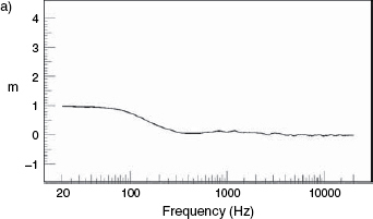
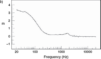
Figure 9.21 Acoustic source plots

Acoustic source plots of the same two loudspeakers whose waterfall plots were shown in Figure 9.8, showing that not only does the reflex enclosure (b) exhibit a longer decay than (a), but also that the low frequencies from loudspeaker (b) effectively emanate from a point over 3 metres behind the physical position of the box. The low frequencies emanate from an apparent point only one metre behind the sealed box (a)

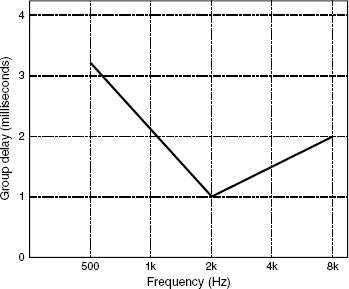
Figure 9.22 The Blauert and Laws criteria for the perception of group delays

Many manufacturers refer to the Blauert and Laws criteria, shown in Figure 9.22. Blauert and Laws determined their results from listening tests, and concluded that any acoustic source plots falling below the line would not be audibly distinguishable in terms of group delay, alone. However, group delays never occur alone, so assumptions about such things should be made with great caution. Effectively the steeper the low frequency roll-off for any given 3 dB down point, the greater will be the group delay and the further behind the physical source will be the apparent source of the low frequency content of a sound.

In some publications the acoustic source has been referred to as the ‘acoustic centre’, but that term is now generally agreed to refer to the point on a loudspeaker front baffle which most closely corresponds to the measurement axis on which the arrivals from the single or multiple drivers would arrive with the most coherent phase relationship. (See sub-Section 9.2.1.)

9.2.7 Cepstrum analysis

The word cepstrum is an anagram of spectrum. Cepstrum analysis results in plots shown in terms of time against non-dimensional decibels which quantify the gamnitude (an anagram of magnitude). In the world of the cepstrum, phase becomes saphe, high pass filters become long pass lifters, harmonics become rahmonics. Power cepstra were developed in the early 1960s for the enhancement of the detection of echoes from earthquakes in vibrationally noisy environments⁹. The repeated signals become more evident after the inverse Fourier transform of the logarithmic power spectrum, which effectively treats the spectrum as though it were a waveform. Figure 9.23 shows a series of pressure amplitude responses of a loudspeaker with a discrepancy between the on and off-axis responses in the region around 5-8 kHz, where the on-axis irregularities are not present in the off-axis responses. The cepstrum analysis shown in Figure 9.24 shows a reflexion around 0.4 milliseconds (400 microseconds), which suggests that the problem is one of diffraction from the cabinet edges at a distance of about 7 cm from the centre of the tweeter. One millisecond represents 34 cm at the speed of sound. Four hundred microseconds therefore represents 34 × 0.4 cm, or 13.6 cm. The half distance, there and back would be 13.6 ÷ 2, or 6.8 cm, and the centre of the tweeter was, in fact, about 7 cm from the top and one side of the cabinet.

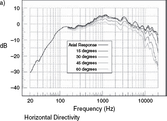
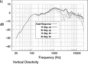
Figure 9.23 On and off-axis pressure responses

Above 4 kHz there can be seen response irregularities in the on-axis response which are not evident in the off-axis responses

Cepstrum analysis is not therefore something which directly relates to what we hear (which is not surprising considering its abstract nature) but it can be a powerful tool for diagnosing the sources of complex problems (which is also not surprising considering its original application).¹⁰

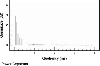
Figure 9.24 The power cepstrum

A strong, single reflexion is evident at about 400 ms, indicating a diffraction problem with the loudspeaker represented in Figure 9.23

9.2.8 Modulation transfer functions

The ubiquitous ‘frequency response’ plots show the pressure amplitude which a loudspeaker generates at each frequency, or in each defined frequency band, in response to a flat input signal. In many cases, as will be shown in Chapter 11, this simple pressure measurement may fail to reveal many other measured response and sonic differences between loudspeakers. Taken to an extreme, we could scramble the overall phase response by measuring a loudspeaker in a reverberation chamber, and adjust it to give a flat response, but the intelligibility of speech or the resolution of detail in music would be hopelessly lost.

For this reason, in reverberant spaces such as railway stations and airport terminals, a measurement of intelligibility known as a speech transmission index (STI) is often employed which is used to indicate the clarity with which the spoken word would be likely to be heard amongst the background noise and reverberation. Using similar techniques, a system of modulation transfer function (MTF) measurement can be used to indicate the degree of accuracy with which a loudspeaker is reproducing the information content in a musical signal.

Thought of another way, imagine a frequency response like a letter-count in this paragraph. We could individually count all the numbers of the letters a, b, c, d etc, and end up with a table such as a = 28, b = 9, c = 13 etc. If we then shuffled the letters around into one giant anagram, a subsequent letter count would still provide the same result as before; a = 28, b = 9, c = 13 etc, but depending on the degree to which we mixed up the letters, the information content of the paragraph would gradually be lost.

When resonances or group delays within loudspeaker systems or their crossovers and amplifiers smear the time response of a signal, a flat pressure amplitude response may still be achievable, but the onsets of all the components of the music will not arrive in the correct temporal order. They will all arrive, but out of sequence due to phase response errors, so an information content loss would be experienced which would equate to shuffling letters around in a paragraph. Fine detail in the musical sounds would be lost, and the jumbled signals would produce other artefacts which were not a part of the original signal. In Chapter 11 is a discussion of the application of this concept to loudspeaker box tunings and port resonances, but here it may be interesting to see how this MTF concept can be applied to room acoustics.¹¹

Figure 9.25 shows the comparison of results from a high resolution, full range, flush-mounted monitor system, at a distance of one metre and four metres in the highly damped control room of a music recording studio. The MTF measures the accuracy of response, frequency by frequency, in terms of its fidelity to the input waveform – ‘1’ being perfect and ‘0’ representing no similarity between input and output. It is evident from Figure 9.25 that the control room is not giving rise to any significant loss of information content as the sound waves cross the room, because there is very little difference between plots (a) and (b). [And no; despite the oft heard criticisms about absorbent rooms being oppressive, the room is not oppressive to be in because there is plenty of reflective surface area sited where the loudspeakers cannot ‘see’ it, but where it can add adequate life to the speech and movements of people within the room.]

The tests were then repeated using a pair of small loudspeakers in a studio recording/performing room having a relatively neutral acoustic character. Figure 9.26 shows the results, and it can be seen how the MTF drop (information loss) from 1 metre to 4 metres is clearly apparent. Figure 9.27 shows the results of moving the tests into a granite-walled, acoustically live room, using the same loudspeaker and microphone as for Figure 9.26. It is plainly apparent that even at a distance of only one metre, the response has already been significantly degraded with respect to the one metre measurements in the more neutral room. It is also apparent from Figure 9.25 how the full-range, high-resolution, flush-mounted (and expensive) professional monitor system shows more generally detailed information content (a higher MTF at all frequencies) than the small, inexpensive, yet popular ‘studio monitor’ used for Figures 9.26 and 9.27.

9.2.8.1 Application of room equalisation

A number of companies are now offering monitor systems which purport to deal with the room problems by means of active or adaptive equalisation, to restore a flat frequency response even in relatively uncontrolled rooms.

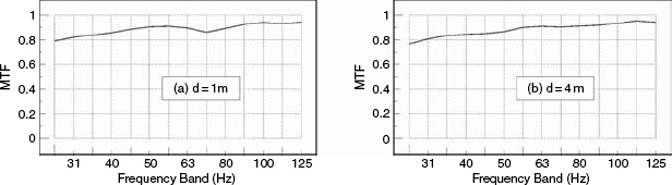
Figure 9.25 Flush-mounted, full-range monitors in a control room

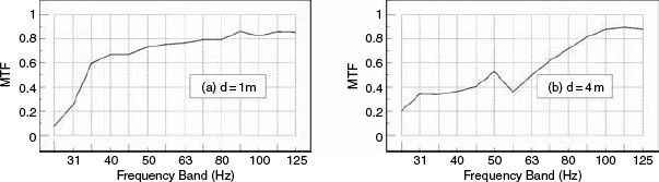
Figure 9.26 Small loudspeakers in a studio performing room

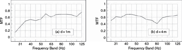
Figure 9.27 Small loudspeakers in a granite-walled, live room

The implication from the publicity often seems to be that room acoustic problems can now be dealt with by signal processing, and also that the highest standards of monitoring clarity can be achieved in less than well-acoustically-designed rooms.

In general, the phase response of a room/loudspeaker system can be separated into minimum-phase (-shift) and excess-phase (-shift) components, as discussed in Section 7.9. The minimum-phase components of the response are given rise to by anything which affects the response in a more or less instantaneous way – such as the extra loading on the diaphragm, and the consequent bass boost, when a loudspeaker is placed in a corner. Excess phase effects result from time-shifted events, such as group delays in crossover outputs (where the high frequency and low frequency outputs of the filters suffer different signal delays) or reflexions which interfere with a loudspeaker response after returning from a distant surface. In the case of any minimum-phase response modification, the amplitude equalisation will automatically tend to correct the phase errors, and hence the time response (transient response) will also be improved. On the other hand, an excess-phase response will often not have its phase response improved as the amplitude response is flattened, and so its transient response may even be made worse due to time smearing as the amplitude component of the frequency response is flattened.

Figure 9.28 shows the MTFs for the wide-range, high resolution monitor in the highly-damped control room (as shown in Figure 9.25). In this case, its response has been flattened in a computer by the application of a ‘perfect’ real-time filter, which also employed a 12 dB/octave filter below 20 Hz to prevent wild, out-of-band correction responses. In terms of the MTF, little has changed between Figures 9.25 and 9.28, either at one metre or at four metres. The average MTF has not changed. In the case of Figure 9.29, however, which shows the result of ‘perfect’ real-time equalisation to the smaller loudspeaker in the well-controlled studio room, (as shown previously in Figure 9.26) the MTF response at one metre has been significantly improved by the equalisation, but the response at four metres distance has hardly been improved at all. The results for the same loudspeaker in a stone room, after equalisation to flatness, are shown in Figure 9.30, where it can be seen that the MTF response has also been improved at one metre, but the response at four metres has barely been affected.

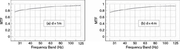
Figure 9.28 Large loudspeakers in a control room – after correction

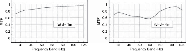
Figure 9.29 Small loudspeakers in a performing room – after correction

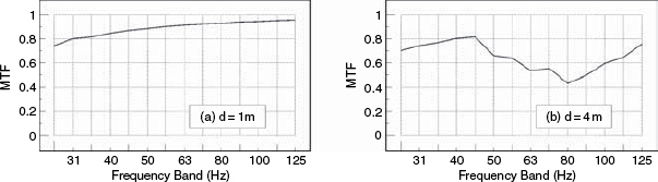
Figure 9.30 Small loudspeakers in a granite room – after correction

These results suggest that the new breed of room-equalised loudspeaker systems can work well at short distances, but that the far-field response in the room may/will not benefit in terms of the resolution of detailed information content, even though the frequency response may appear to be quite flat. In other words, such equalisation may improve the sound for the person close to the loudspeakers, but on the sofa a few metres away the MTF response may remain as bad as ever, or worse! It would appear that only well-designed room acoustics can provide and maintain a large, flat, high-resolution listening area.

All rooms, unless highly absorbent, affect the transmission of information from a loudspeaker to a listener, and even at low frequencies the loss of information content (detail) can be significant. In well-designed listening/control rooms of low decay time (which, once again, need not be oppressive to be in if reflective surfaces are strategically placed) the loss of information content is minimal. However, the overall responses in less well treated rooms can be improved considerably by modern equalisation processes, but only, it would seem, at relatively short distances from the loudspeakers. Room equalisation does not, in general, significantly reduce the loss of signal information at greater distances.

What the evidence presented here is highlighting is that the flattening of the ‘frequency response’ is not necessarily restoring low level detail and low frequency information accuracy. In fact, as the amplitude part of the frequency response is being flattened, the phase response may be suffering degradation. This may make it easier to achieve a correct musical balance for a mix, but it may not do anything to improve the assessment of things such as the fine structural detail or the transparency of the room sounds within the recordings.

Once we get into the lower MTF regions at low frequencies, experience has shown it can become more difficult to balance percussive and more continuous sounds, such as bass guitar to bass drum balances. A good MTF and a fast transient response at low frequencies therefore remain essential features of a good mixing environment.

Clearly, this type of insight into loudspeaker and room responses requires techniques such as MTF analysis in order to be able to confirm and see what ears have been telling people for decades, but which many ‘conventional’ established forms of loudspeaker measurement systems have signally failed to reveal.

9.2.8.2 A D-to-A dilemma

A further point should also be raised about mid-priced loudspeaker systems which incorporate digital equalisation. The quality of the D to A converters should be considered when thinking about using them. A good quality pair of D to A converters for monitoring a recording made via good quality A to D converters costs around 1000 euros/dollars or more. Clearly, on entire loudspeaker systems costing only 1000 euros/dollars, and having digital inputs, the converters used in the electronics will probably cost nearer to tens of dollars. When auditioning different converters using these loudspeakers, this situation could (and in fact does) lead to conclusions such as: “When we made comparisons, the mid-price A to D converters sounded just as good as the super-expensive ones”. Such conclusions could easily be drawn when monitoring via mid-price monitor systems which use digital equalisation systems and low-cost D to A converters in acoustically untreated or inadequately treated rooms.

John Watkinson raised this issue when he suggested that the resolution of a loudspeaker system could be tested by reducing the bit rate of a digital signal until the loss became noticeable¹². The loudspeakers making audible the smallest bit-rate reductions being the ones with the greatest resolution of fine detail. Although some holes can be picked in this argument, the basic concept does seem to hold water. In practice, the problem which this highlights is that if the limitations of the D to A conversion of the monitor system, or poor MTFs due to bad room acoustics, lead to bad decisions about the choice of A to D converters, the deficiency will be forever locked into the recording. Conversely, excellent A to D conversion, even if not revealing itself on all reproduction systems, will be fully enjoyable by those who do listen to the recordings via high quality reproduction chains. However, measurement systems for accurately predicting subtle sonic differences in A-to-D and D-to-A conversion are still not well-defined, and no simple, powerful tool is yet readily available. Nevertheless, it should be rather self-evident that if any D to A converters in the monitor system are not of the highest quality, then they will limit the ability to monitor the quality of any other converters in the recording chain. Cheap, quality-control monitors with digital inputs are therefore, effectively, a contradiction in terms.

9.3 Sound fields and human perception

Once all the objective testing has been completed, the ultimate assessment of the quality of a loudspeaker intended for musical use must be made by the ear. Unfortunately there are some aspects of perceived loudspeaker quality which do not easily lend themselves to objective measurement, yet which are important aspects of perceived quality. No matter how good a recording may be, and no matter how good its reproduction in terms of spacial imaging and definition, one incontrovertible fact is that its reproduced sound-field will bear little resemblance to the sound-field of the original instrument. Of course, if the music is an electronically based creation, where no real instruments ever existed other than the electronic system itself, then the loudspeaker playback on the original monitor system on which it was mixed is the definitive sound field. However, a loudspeaker reproduction of a cello recording will inevitably give rise to a huge spacial distortion in terms of the sound field. A bowed cello radiates sound from a large area, and in a very complex manner. Walking round a cello whilst it is being played, a listener may experience a small reduction in the high frequencies when passing immediately behind the cellist, whose body will tend to cast a high frequency shadow, but otherwise the tone would be perceived to be relatively independent of position. The source is very distributed, with many parts of the instrument radiating a wide range of frequencies at the same time. The sound field pattern from the instruments contrasts sharply with that from any loudspeakers radiating a reproduction of a recording of the same instrument.

The recording microphone is a pressure transducer, or a pressure gradient transducer if of figure-of-eight pattern, which responds to the radiated sound received at the small place that the diaphragm occupies, and converts the sound pressure changes into an electrical signal. In stereo, with two microphones, a two-channel signal can be recorded which can convey to the ear of a centrally placed listener, via loudspeakers or headphones, enough information to give a sensation of the source positions in terms of left and right, but not in terms of height. Once these signals are reproduced via multi-driver loudspeakers, the ‘no-height’ information is also separated into frequency bands. All the high frequencies above a certain crossover point will come from two points (the tweeters), perhaps no more than 3 cm in diameter, spaced at the extreme left and right of the sound-field. The composite high frequency sound pressure is thus beamed at the two ears in two separate rays, from two points in space, with no height information.

Compare this to listening to the instruments of a string quartet or a rock group. The sound sources are multiple and are distributed in width and height. High frequencies arrive from the entire drum kit, with the cymbals above ear height and the snare drum below, or with the violin above and the cello below. If the recordings were made in an anechoic chamber, then played back in a reflective room, comparison to the live performance at the same place in the same room would show many differences. The real instruments would each be located at different places with regard to the nodes and anti-nodes of the room modes. Conversely, the phantom images of the recorded instruments would all originate only from the two loudspeaker positions, and only the nodes and anti-nodes relevant to the two places occupied by the two loudspeakers could affect the overall response. A phantom central image of a guitar would not couple to the room at its phantom position, but at each loudspeaker position. Therefore a pair of loudspeakers would send a signal to the ears from two places, whereas a real group of musicians would send their sound to the ears from many individual positions. In reflective/reverberant conditions, a pair of loudspeakers would couple to the room acoustics at only two places, whereas a group of musicians would each couple to the room in a different way, and even the individual drums in a kit would couple differently to the room modes, and each produce their own unique reflexion patterns and timings. Given the extreme sophistication of the human hearing system it would be stretching the imagination to even hope that such differences between live music and music reproduced via loudspeakers could go unnoticed.

[The pinnae of the ears (the ear flaps) are highly refined devices which collect sound in different ways from different horizontal and vertical directions. The sound pressure differences at the entrances to the ear canals are therefore not merely the differences that would occur if microphones were placed in the same location in the absence of a head, torso and pinnae. A pair of ear canals receives cues about the directions of sounds in the horizontal and vertical planes which are not available to a pair of microphones, and as such the composite responses are not the same. By the use of dummy heads with ear flaps, binaural recordings of great spacial sensitivity can be made for playback over close-fitting earphones, but such recordings will not work via loudspeakers because the head, torso and pinnae of the listener would introduce a second set of processing which would confuse the delicate information in the binaural recording.]

The ears therefore receive a different set of cues from the distributed set of sources than from a phantom sound stage created by two sources, and the resulting sound-field distortion can lead to great perceptual differences. As loudspeakers cannot three dimensionally reproduce the reality of a live performance, we must therefore look at loudspeaker reproduction as a performance in its own right. The question then to be asked is how well the loudspeakers can transmit the emotions which were generated by the original performance. Given that the musicians were likely to be using the tones of their instruments to manipulate the sensations which they were intending to convey, it would seem obvious that their timbral subtleties should be preserved as accurately as possible. However, exactly how that timbral fidelity can be achieved may depend on certain compromise decisions, but the optimum compromise for one set of instruments may not be optimum for a different set of instruments. The compromises for large loudspeakers with great source areas may be different from the compromises which seem most apt for smaller, more compact sources, but even the differences between those sources may be dependent on the musical genre. Furthermore, to create an appropriate rendition of any given piece of music in different room acoustics may also favour one set of loudspeaker design compromises over another.

When music is created by electronic or electric sources, it is itself created on loudspeakers for reproduction by loudspeakers. One presumes that the loudspeakers on which the music is finally mixed are the reference for the timbre and balance of the instruments, but the question arises as to how to choose those loudspeakers. Are they to be chosen to give the widest range of options for the recording personnel, or are they to be chosen to be the most appropriate to enable the widest range of likely domestic loudspeakers to reproduce the intentions of the producers in the majority of circumstances? This dilemma often leads to the use of different recording and mixing loudspeakers, as was discussed in Chapter 8.

There are in fact some market tendencies which do exist. Leaving aside the audiophiles for now, and also leaving aside the people for whom music is just something to fill the empty air, there is a tendency, for people who choose their loudspeakers by careful listening before buying, to choose different loudspeakers depending upon the type of music that they mostly listen to. People who like orchestral music tend to buy different loudspeakers to those who like rock music. In fact, there is also a tendency for recording engineers who work principally with classical music to use different monitor loudspeakers to those who record rock music. What is more, there are traceable similarities between the recording/mixing and domestic listening loudspeakers used by each group.

The orchestral/acoustic music listeners tend to value loudspeakers with low non-linear distortion, low colouration and a smoothly rolling-off low frequency response, coupled with wide and smooth directivity to give rise to plenty of the lateral reflexions which are necessary to produce a sense of spaciousness. Pinpoint stereo positioning is often low on their agenda, because in the reflective and reverberant acoustics of a concert hall, no precise positional localisation is possible at a live concert; and neither is it usually considered to be desirable, because it would imply an acoustic that could not support the spaciousness – the two things are generally mutually exclusive. On the rock music side, flat low frequency responses are often valued, even if they cut-off quite abruptly. Colouration is to some degree acceptable because instruments are often so heavily equalised in the recording and mixing processes that no real reference exists. Heavy percussion and transient signals are commonplace, so high sound pressure level capabilities are often required, and as the audibility of small amounts, or even not so small amounts, of non-linear distortion is doubtful on such high impact recordings, non-linear distortion levels may be tolerable which would be too high for classical music enthusiasts. Relatively narrow directivity may also be deemed to be desirable for rock music enthusiasts because too many room reflexions can detract from the transient impact of the fast changing music. However, all of the above-above-mentioned items are tendencies, only, and will not apply in all circumstances.

Of course for a price, if money is no great object, very many of the most desirable properties could be reasonably incorporated into one design, but it would not be cheap and it would not be small. At 2006 prices, if one were prepared to pay 2000 euros per pair of 50 litre boxes, one could begin to approach a compatible design if the room acoustics could also be reasonably contoured to requirements. Unfortunately though, it is sad to say that even people in some supposedly professional parts of the music industry consider such costs and sizes to be beyond their circumstances. In such cases, it is really important to understand that when compromises are made when using cheaper and smaller loudspeakers, they may not be as suited to some music or rooms as they are to others, so any reference which they provide may not be as robust or broad-based. Further implications of mix compatibility will be discussed in Chapter 10, but in general, within reason, as loudspeaker costs and sizes increase, and rooms become better controlled, the easier it is to achieve a more universal set of monitors. Small, cheap loudspeakers, if they are good at all, tend only to be good for a limited range of circumstances and uses.

It is therefore difficult to be too rigid in trying to determine threshold levels for ‘good’ performance when considering the implications of the various characteristics discussed in Section 9.2 because what is optimal for any given size of loudspeaker will depend upon its use. Ultimately, the goal of listening to music is to enjoy it, so what gives pleasure has value, even if it can be technically argued against. However, in general, the closer that one can get to technical excellence, the overall sonic performance of a loudspeaker usually improves, and it is surely incumbent on a professional recording industry to be fully aware of what is on a recording, even if 99.9% of the purchasers of the end products are not going to hear the subtleties. The music buyers can invest in their domestic entertainment systems according to the degree that they are important in their lives, but professional attitudes are more demanding. If nothing else, professional pride requires that the end users should not become aware of recording errors that passed unnoticed through the recording and mixing process.

9.3.1 Further perceptual considerations

The fact that our pinnae, middle ears, inner ears and brains are unique to each of us introduces aspects of physiology and taste into the questions of loudspeaker parameter optimisation. Culture and ethnicity also have a bearing on the subject. When concentrating on listening to music, all human beings tend to react with the side of the brain which relates to them being right or left handed. When listening in a relaxed way, the tendency is for the activity to switch to the opposite hemisphere. Mongoloid races, such as Japanese, tend to process western music with one half of the brain and oriental-style music with the other half of the brain¹³.

Dr Diana Deutsch, at the University of San Diego, California, published finding showing that the place of our birth, irrespective of being from local descendants or not, can affect our musical perception. The median pitch of the language and accent with which we first learn to speak can fix certain aspects of our musical perception for the rest of our lives, and may even affect the perception of complex pitch sequences in terms of whether we hear them to be rising or falling¹⁴. Southern English and Californian populations were shown to perceive a tri-tone pitch sequence in opposite ways. During listening tests at the Institute of Sound and Vibration Research, a band-limited, anechoic recording of an acoustic guitar chord was perceived by some listeners to change its notational inversion when played through different loudspeakers, whilst other listeners heard the same chord notation but a change in the timbre¹⁵.

During the installation of a monitor system in London in the late 1980s, there arose a situation with two well respected recording engineers who could not agree on the ‘correct’ amount of high frequencies from a monitor loudspeaker system which gave the most accurate reproduction when compared to a live cello. They disagreed by a full 3 dB at 6 kHz, but this disagreement was clearly not related to their own absolute high frequency sensitivities because they were comparing the sound of the monitors to a live source. The only apparent explanation for this is that because the live instrument and the loudspeakers produced different sound fields, the perception of the sound-field was different for each listener. Clearly, all the high frequencies from the loudspeaker came from one very small source, the tweeter, whilst the high frequency distribution from the instrument was from many points on the strings and various parts of the body. The ‘highs’ from the cello therefore emanated from a distributed source having a much greater area than the tweeter. Of course, the microphone could add its own frequency tailoring and one-dimensionality, but there would seem to be no reason why this should differ in perception from one listener to another.

During research in the late 1970s, Belendiuk and Bulter¹⁶ concluded from their experiments with 45 subjects that “there exists a pattern of spectral cues for median sagittal plane positioned sounds common to all listeners”. In order to prove this hypothesis, they conducted an experiment in which sounds were emitted from different, numbered, loudspeakers, and the listeners were asked to say from which loudspeaker the sound was emanating. They then made binaural recordings via moulds of the actual outer ears of four of the listeners, and asked them to repeat the test, via headphones, of the recordings made using their own pinnae. The headphone results were very similar to the direct results, suggesting that the recordings were representative of ‘live’ listening. Not all the subjects were equally accurate in their correct choices, though, with some, in both their live and recorded tests, scoring better than others in terms of identifying the correct source position. Very interestingly, when the tests were repeated with each subject listening via the pinnae recordings of the three other subjects in turn, the experimenters noted, “that some pinnae, in their role of transforming the spectra of the sound-field, provided more adequate (positional) cues than do others”. Some people who scored low in both the live and recorded tests, using their own pinnae, could locate more accurately via other peoples’ pinnae. Conversely, via some pinnae, none of the subjects could locate very accurately. However, for all the subjects, listening through their own pinnae sounded most natural to each of them.

Interestingly, some people do claim to hear height information in two-channel stereo recordings which can carry no such information, but this is an effect of their own pinnae being stimulated in different ways by different loudspeakers and mounting conditions. Such people really do hear height in the stereo images, but only as an artefact of their own pinnae, and not of the recordings or the loudspeakers.

Given these differences, and all of the aspects of frequency discrimination, distortion sensitivity, spectral response differences, directional response differences, psychological differences, environmental differences, cultural differences, and so forth, it would be almost absurd to expect that we all perceive the same balance of characteristics from any given sound. True, whatever we each individually hear is natural to each one of us, but when any reproduction system creates any imbalance in any of its characteristics, as compared to a natural event, the aforementioned human variables will inevitably dictate that any shortcomings in the reproduction system may elicit different opinions, vis-à-vis the accuracy of reproduction, from different people. So, to the question of whether it is more important to reduce the harmonic distortion in a system by 0.2%, or the phase accuracy by 15 degrees at 15 kHz could well be an entirely personal matter, which could be task related, music related or room related, or even related to a person's psycho-physical make-up.

In fact, it could also be experience related. Human beings have a great tendency to acclimatise themselves to familiar sounds. If we go into a strange house, we often note the change in the sound of our voices, yet in our own homes we rarely notice a change from going from outside to inside, because we are so used to it. People who have been working for years on a certain genre of loudspeaker also have a tendency to hear music in relation to the way that they are accustomed to hearing it. It is hard to say whether people make some choices about loudspeakers because they suit their concept of what sounds right to them, or because they have a recognisably familiar sound that they feel comfortable with. In the realms of acoustic music, if a listener is also a regular concert-goer, the reference of the general sound of live instruments is always in the back of their mind as a reference, but with heavily processed music, only the people in the control room at the time of the mixing really know what the sound should be like. People can and do get accustomed to how a wide range of non-acoustic music sounds on their own loudspeakers, then presume that that is how everything should sound. [Conversely, I had a recording which I liked very much and had played it on many systems, the better ones of which yielded a remarkably rich yet obviously natural drum sound. By chance, several years later, and on a different continent, I met the mixing engineer, and told him what I thought of the recording. “Natural?”, “I had to e.q. the hell out of it to get that sound!” he exclaimed. So we have to be very careful about our supposed references. P.N.]

Despite all of the complications of human perception, objective analysis of loudspeakers is fundamental for keeping the progress on the rails because subjectivism has far too many variables. Toole speaks of a circle of confusion¹⁷, where recordings considered to be ‘good’ are used to assess loudspeakers, which are used to make recordings, which are made to assess loudspeakers, which are used to make recordings ad infinitum.

If this is done in conjunction with continued reference to objective loudspeaker measurements, it is perhaps one of the only means that we have to refine our assessments, but Toole's implications were that this has often been a ‘circle of testing’ which has occurred too often without the strict objective constraints. Where, for example, domestic loudspeakers of average quality have been the de facto reference, and monitoring loudspeakers have been chosen which give the best compatibility with this arbitrary reference. Then the new sounds recorded via this system become the reference recordings, and so forth. Some marketing people may actually applaud this, but professionally it is a loose practise.

Moulton¹ discusses listening in the living room, the bedroom, the car, on headphones, on the ‘ghetto blaster’ in the street, then concludes that in order to sound compatible on all these irreconcilably different playback systems, a recording must be:

a)	comparatively simple spacially and texturally
b)	limited in note-to-note dynamic range
c)	exaggerated in spacial characteristics that do not become significantly degraded timbrally when summed into mono and,
d)	must not depend on their musical effect for any frequencies outside of a range from 80 Hz to 10 kHz

The latter requirement dispenses with three whole octaves of the audible range – octaves where the ‘power’ and ‘air’ are to be experienced. Even people who cannot hear tones above 10 kHz can still usually hear when the 10 to 20 kHz band is cut, so if we were to monitor only to this lowest common denominator, we would be robbed of much of the musical experience when listening on audiophile systems. Working like this does no justice to either the art, the technology or the science. The discerning listeners deserve more.

Whilst the 80 Hz to 10 kHz brigade are unquestionably the bread and butter of the industry, the artistes, the dedicated professionals and the audiophiles are the great driving force that keeps it fresh and interesting. Said Roederer, “Music is not a waveform, but a psychological and spiritual construct within the mind. The waveform and its physical dimensions are simply carriers of musical information”¹⁸. Yet, that waveform is best defended from corrupting influences if the objective performance of a loudspeaker is designed to best convey it. Despite the subjective assessment being the ultimate arbiter of any loudspeaker's performance, it is only by objective means that we can keep focussed on the engineering targets, without which, and by subjective means only, we would surely become lost.

It may well be that the dynamic ebb and flow of the music, the subtle timing differences and other characteristics are better exhibited by some loudspeakers than by others, but these are things for which we have no reliable, measurable descriptors. However, the overwhelming tendency is for a loudspeaker which scores highly in all the objective measurement regimes detailed in Section 9.2 to show the musical characteristics in a more artistic and exciting light. Nevertheless, it must always be the case that until we have perfection, we will always be faced with different balances of compromises serving some situations better than others.

References

1  Moulton, D., ‘The Creation of Musical Sounds for Playback Through Loudspeakers’, AES 8^th International Conference, The Sound of Audio, Washington DC, USA (1990)

2  Watkinson, John; ‘The Jitter Bug’, Resolution, Vol 1, No 4, UK (October 2002)

3  Briggs, G., ‘Sound Reproduction’, Third Edition, p 174, Wharfedale Wireless Works, Bradford, UK (1953)

4  Newell, P., Holland, K. R., ‘Do All Mid-Range Horn Loudspeakers have a Recognisable Characteristic Sound?’ Proceedings of the Institute of Acoustics, Vol 12, Part 8, pp 249–258, Reproduced Sound 6 conference, Windermere, UK (1990)

Also in: Newell, P., ‘Studio Monitoring Design’ Chapter 12, p 200, Focal Press, Oxford UK (1995)

5  Czerwinski, E, Voishvillo, A., Alexandrov, S., Terekhov, A., ‘Multitone Testing of Sound System Components – Some Results and Conclusions, Part 1: History and Theory’, Journal of the Audio Engineering Society, Vol 49, No 11, pp 1011–1048 (November 2001)

6  Czerwinski, E., Voishvillo, A., Alexandrov, S., Terekhov, A., ‘Multitone Testing of Sound System Components – Some Results and Conclusions, Part 2: Modeling and Application’, Journal of the Audio Engineering Society, Vol 49, No 12, pp 1181–1192 (December 2001)

7  Voishvillo, A., ‘Assessment of Loudspeaker Large Signal Performance – Comparison of Different Testing Methods and Signals’, Presented at the 111^th AES Convention, New York, USA (November/December 2001)

8  Janovsky, W., ‘The Audibility of Distortion’ (in German), Elek, Nochr.-Tech, Vol 6, pp 421–430 (Nov 1929)

9  Bogert, B. P., Healy, M. J. R, Tukey, J. W., ‘The Quefrency Analysis of Time Series for Echos: Cepstrum, Pseudo-Autocovariance, Cross-Cepsrum and Saphe Cracking’, in Rosenblatt, M., (editor), Proceedings of the Symposium on Time Series Analysis, pp 209–243, Wiley, New York, USA (1963)

10  Holland, K. R., ‘Use of Cepstral Analysis in the Interpretation of Loudspeaker Frequency Response Measurements’ Proceedings of the Institute of Acoustics, Vol 15, Part 7, pp 65–72 (1993)

11  Holland, K., Newell, P., Castro, S. and Fazenda, B., “Excess Phase Effects and Modulation Transfer Function Degradation in Relation to Loudspeakers and Rooms Intended for the Quality Control Monitoring of Music”. Proceedings of the Institute of Acoustics, Vol 27, Part 8, Reproduced Sound 21, (2005)

12  Watkinson, J and Salter, R., “Modelling and Measuring the Loudspeaker as an Information Channel”, presented to the ‘Reproduced Sound 15’ conference of the Institute of Acoustics, Stratford-on-Avon, UK (November 1999)

13  Davis, D., Davis, C., ‘Sound System Engineering’, Second Edition p 9, Focal Press, Oxford, UK (1997)

14  Deutsch, D., ‘Paradoxes of Musical Pitch’ in Scientific American, Vol 267, No 2, pp 70–75 (August 1992)

15  Newell, P., ‘Studio Monitoring Design’ Chapter 5, Section 5.6, Focal Press, Oxford, UK (1995)

16  Belendiuk, K., Butler, R. A., ‘Directional Hearing under Progressive Impoverishment of Binaural Cues’ Sensory Processes, 2, pp 58–70 (1978)

17  Toole, F., ‘Art and Science in the Control Room’ Proceedings of the Institute of Acoustics, Vol 25, Part 8, Reproduced Sound 19 conference, Oxford, UK (2003)

18  Roederer, J. G., ‘Introduction to the Physics and Psychophysics of Music’ 2^nd Edition, pp 11–12, Springer Verlag, New York, USA (1979)

Bibliography

1  Voishvillo, A., ‘Assessment of Nonlinearity in Transducers and Sound Systems —From THD to Perceptual Models’, presented at the 121^st convention of the Audio Engineering Society, San Francisco, USA (October 2006)