
Chapter 6
Effects of amplifiers and cables
Clearly, no loudspeaker can do its job unless it is connected to a suitable power amplifier, and to make that connection, an appropriate cable is required. As no cable can improve any signal which it is passing (unless it is filtering out some other problem that should not be there) it must be concluded that the best cable is no cable. Moreover, as no amplifier can improve the accuracy of the signal which it is passing, the only conclusion which can be drawn is that the combination of amplifier and cable can only degrade the signal. However, as we must use an amplifier and a cable, art and science are both employed in order to minimise the inevitable degradation.
Well, at least that is the situation as far as accurate monitoring is concerned. In the case of amplifiers which are used for musical instrument amplification, the amplifier is actually a part of the instrument, so whatever sounds right is right. The gross distortion produced by an old, valve, Leslie tone-cabinet, when amplifying a Hammond organ beyond the point of overload, was one of the most emotive sounds in the history of rock music, but we will come to that in Chapter 8. Similarly, the popularity of valve amplifiers in many domestic hi-fi systems is widely attributed to the pleasing ‘musical’ sounding even harmonics which they tend to produce. Again, this will be discussed further in Chapter 8, but as these effects are totally subjective in terms of their desirability, it is very difficult to deal with the subject in any definitive way. Therefore, what we will attempt to do in this chapter is look at the problems of amplifiers and loudspeaker cables when accuracy of reproduction is the goal, and which we can deal with in an objective manner.
6.1 Amplifiers – an over-view
The purpose of a power amplifier is to take a voltage signal, usually in the order of up to one or two volts peak, and deliver the waveform of that signal in a way that a proportionally larger voltage can be supplied to drive current through a loudspeaker motor system. This, in turn, is used to generate a radiated acoustic output which is also the best replica possible, in terms of pressure fluctuations, of the input signal to the amplifier. Driving power into a resistor is a reasonably simple exercise, but driving the signal into a load similar to that shown in Figure 1.7 is a different matter. Driving power into a load such as that shown in Figure 6.1, an electrostatic loudspeaker,can be an even more difficult problem to overcome, because the first thing that an amplifier ‘sees’ is a large capacitor across its output terminals. As explained in the previous chapter, the current and voltage are not in phase when passing through loads which are predominantly either inductive or capacitive.
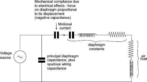
Figure 6.1 Load impedance presented by an electrostatic loudspeaker
Traditionally, power amplifiers have been rated into resistive loads. This makes sense, even though it is unrealistic, because there is no standard loudspeaker load – the range of variability is just too great – but driving a loudspeaker nevertheless tends to be very different from driving a resistor. There was, and perhaps still is to some extent, an objectivist lobby who claim that all well-engineered amplifiers exhibiting adequate output power and minimal distortion will sound identical. In the opinions of the authors of this book, this is absolutely not the case. Amplifiers do sound different, at least once they can be heard through high resolution loudspeakers in well controlled rooms. Undoubtedly, part of the reason why they sound different is due to their performance when driving loads which are typically represented by Figures 1.7 and 6.1, although numerous other factors also play their parts.
An interesting incident occurred at the Tannoy factory in Scotland1, in the early 1990s, where a group of people of some repute in terms of their auditory acuity were assembled to select an amplifier to offer as standard with a new range of loudspeakers. There were four loudspeakers in the range, and four different amplifiers had been short-listed for audition. The intention was to select one amplifier from the four. However, in the blind tests, one amplifier was selected as sounding most accurate on one of the loudspeakers, another amplifier was chosen for another loudspeaker, and a third amplifier was deemed to sound most accurate on the remaining two loudspeakers of the range. The loudspeakers in question were all of similar design concept, but varying in size. The participants in the tests were all highly experienced and respected engineers, and all had been expecting that they would choose one amplifier for the whole range of the loudspeakers.
It could have been the case that certain characteristics of the individual amplifiers counterbalanced opposing characteristics in the different loudspeakers, and this could also have been due to the different load characteristics presented by each loudspeaker. The component values in terms of the circuit shown in Figure 1.8 could all have been different. However, we do not have anything like a perfect loudspeaker to use as a reference, so it is difficult to say which of two amplifiers is definitely better or worse when the differences are subtle and there is no ‘audible quality meter’ that we can connect to their outputs. In fact, we listen to amplifier/loudspeaker combinations, rather than just to amplifiers, and we can add listening rooms to those combinations in most circumstances. Given the fact that the rooms constrain the air which loads the loudspeaker diaphragms, it can be seen from Figure 1.8 that the rooms will also reflect back their presence into the loading of the amplifiers.
Ultimately, the ear is the only judge, and as it listens to the systems, it often cannot differentiate the sources of some audible effects from the sources of others. We also all have different ears, with different perception of sound, and as no microphone is perfect, we have no perfect sources of sound to compare anything with. To further compound all of this, unlike the optic nerve, which carries a measurable and recognisable signal from the eye to the brain, the auditory nerves disappear into about six different parts of the brain, and our understanding of how the mind puts the whole sound together is still not well advanced.
So just what can we say about amplifiers if they have to perform in such a murky world of variable loading and variable perception? This is a question that we must address in a very careful way if we are not to descend into the realms of misguided subjectivism, which may be appropriate in some circumstances, but which cannot lead to a robust consensus in professional circumstances.
6.2 Basic requirements for current and voltage output
Contrary to much popular thinking, amplifier power should not be matched to the power rating of the loudspeakers or individual drivers to which they are connected. The amplifiers should have a margin of at least 6 dB (four times the power) above the peaks of the highest level that they will be likely to be called upon to deliver. If it is to be presumed (somewhat sarcastically but nonetheless realistically) that most loudspeakers will at some times be used to their limits, then some common sense needs to be applied to their use because this means using amplifiers which can maintain an undistorted output beyond the peak level rating of the loudspeaker. However, the last requirement is not always easy to assess from any simple Ohm's law calculation. The reactive components in the impedance of a loudspeaker can give rise to significant phase shifts between the current and the voltage. If the phase shifts become significant, currents can be drawn which are totally beyond any expectations which would be calculated from the treatment of the load impedance as being largely resistive. Many amplifiers of seemingly adequate power rating have been shown to fail to be able to supply adequate current with difficult loads, even though their voltage headroom has been easily sufficient for their proposed use.
Such amplifiers may be found to be seriously lacking in the quality of sound that they can achieve with a loudspeaker which presents a highly non-uniform impedance to its output terminals, yet many of these amplifiers may be considered to give excellent reproduction when driving a more benign load. In general, it is loudspeakers with passive crossovers which present the greatest problems, at least when we are considering moving coil loudspeakers, but attempts to flatten the impedance curves by the addition of compensation networks in the crossovers has often been found to detrimentally affect the overall sonic performance of the system. In the previous chapter a strong case was made against the use of passive crossovers for very high quality loudspeaker systems, but many popular monitor loudspeakers still use this approach, so the problems which they give rise to still need to be considered.
6.3 Transient response
In the perception of music, the leading edge of a waveform is highly significant for the recognition of instruments. With the leading edges removed it can be difficult to tell the sound of a guitar from the sound of a violin, for example. It follows that the subtle differences between different guitars and different violins – and most other instruments for that matter – can be very dependent upon the accuracy of the transient waveform of the onset of the note. Apart from the need to supply adequate current when a bass drum is played loudly through the loudspeakers, slew rate and frequency response are also important factors. The former is measured in volts per microsecond, and is a measure of the speed with which the output of an amplifier can respond to the input signal. Forty volts per microsecond would be the typical slew rate capability of a good monitoring amplifier, but this same rate needs to be maintained at high levels, and not just at low levels, or slew limiting will occur, which can produce some very odd waveform distortion.
The transient response is also greatly affected by the frequency response of the amplifier. An electrical step function is shown in Figure 6.2. This waveform is also known as a Heaviside function, named after Oliver Heaviside. (Discoverer of the Heaviside layer which surrounds the Earth.) The generalised function is defined by
H(x) = 0 for x < 0
H(x) = 0 for x > 0
Its value at x = 0 is not defined
It is an all or nothing function, also known as a step function, and it contains all frequencies. A battery switched on and off, with a few seconds between switching, is a form of step function generation. If connected to the input of a spectrum analyser, a 1½ volt battery will demonstrate the wide frequency distribution. When connected or disconnected, all the columns of the analyser will be seen to be excited, giving rise to a straight line response with a roll-off of 3 dB per octave relative to the flat response of pink noise.
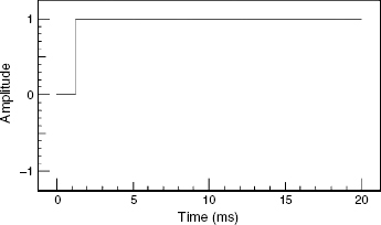
Figure 6.2 Waveform of a step-function (Heaviside function)
If an amplifier has high and low frequency roll-offs which begin too close to the audible frequency extremes, it will exhibit phase shifts as shown in Figure 6.3. The instantaneous onset of the step function requires that all the frequencies begin at time zero. Any phase shifts present in the system will give rise to signal delays, which will smear the waveform. Figure 6.4 shows a step function after passing through an amplifier whose response is 3 dB down at 15 Hz and 30 kHz in (a), then 3 dB down at 30 Hz and 15 kHz in (b), with 12 dB/octave roll-offs in each instance. Rates of change of phase beyond about 5 degrees per octave in the audible range are noticeable to most people, at least when demonstrated on monitoring systems which are themselves relatively phase-accurate. However, many monitor loudspeaker systems have phase responses that are so appalling that they can swamp the audible effects of phase shifts elsewhere in the system, rendering them inaudible, but this can hardly be considered to be ‘monitoring’. In general, it is desirable for a good monitor amplifier to have a flat amplitude/frequency response between around 5 Hz and 80 kHz – two octaves either side of the audible frequency range – if good transient responses are to be expected.
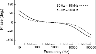
Figure 6.3 Roll-offs and their corresponding phase shifts
Changing phase-shifts associated with different bandwidths. In the case shown, the roll-offs are second order – 12 dB/octave. When the rate of change of phase exceeds about 5 degrees per octave in the audio band, noticeable changes in the timbre of musical instruments become noticeable in high quality monitoring conditions (especially with loudspeakers exhibiting fast transient responses in well-damped rooms)
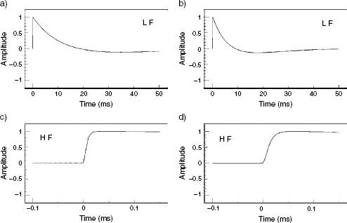
Figure 6.4 Effects of bandwidth on transient responses. Note different time scales
The result of passing the waveform shown in Figure 6.2 through the filtered bandwidths shown in Figure 6.3. The plots (a) and (b) show the decay of the waveform when subjected to second-order roll-offs (12 dB/octave) at 15 Hz and 30 Hz respectively. Note the tendency for the 30 Hz roll-off (b) to overshoot the zero axis as it decays. The effect manifests itself as ‘ringing’, or resonance. The time (transient) response takes longer to return to a flat, zero line than is the case with the 15 Hz response shown in (a)
The plots (c) and (d) show the effect of filtering the response at 30 kHz and 15 kHz respectively. It can clearly be seen how the response filtered at 15 kHz (d) takes longer to rise to its maximum value than in the case of the 30 kHz roll-off shown in (c)
The higher frequency of roll-off at the low frequencies therefore can be seen to extend the decay of a signal, whilst the lower frequencies of roll-off at high frequencies can be seen to extend the attack time of a signal. In either case, as the bandwidth is restricted, the time (transient) response is lengthened
It should be noted that phase shift, however, is something which exists only in the frequency domain, because it is the rate of change of phase with frequency. In the time domain we should speak of the phase slope, which gives rise to the phase distortion that changes the waveform shown in Figure 6.2 to those shown in Figure 6.4. Under good monitoring conditions the transient response of a step function can be heard to change as the bandwidth is reduced. The bandwidth can clearly be demonstrated to have an effect on the attack of a tight sounding bass drum or tom-tom, although, as mentioned above, it takes a good loudspeaker system to show the effects clearly.
This brings us to another ‘chicken and egg’ situation, because when using loudspeakers with poor transient responses the benefits of using a fast responding amplifier may not be appreciated. This can lead to people drawing the conclusion that a wideband response of an amplifier is unnecessary, and reasons may then be found to curtail the bandwidth, applying the philosophy that “the wider the window is opened, the more dirt blows in”. Given the ever-increasing amount of electromagnetic radiation in the atmosphere, there can be a great temptation to filter it out, stage by stage, but the phase shifts through the filters of a recording chain are cumulative. Closing the window unnecessarily in the monitor system is unwise if the monitor system is to be capable of revealing transient problems elsewhere in the system. Maintaining wideband frequency responses throughout the electronic system is very important for maintaining the transient accuracy of the chain.
6.4 Non-linear distortions
Until now we have been speaking about the linear distortions of the amplifiers. A linear distortion involves a change in the waveshape, or the frequency response, but where no new frequencies are introduced that are not present in the input signal. If either the amplitude or phase of the frequency response are distorted, they are linear distortions, and will affect the waveform. Academically speaking, the full frequency response includes both the amplitude and the phase responses, although in more general conversation the term ‘frequency response’ usually simply relates to the amplitude portion, variously known as the magnitude or modulus of the frequency response.
Unlike the linear distortions, a non-linear distortion is one where new frequencies are introduced into the output of a system. In the case of harmonic distortion, these extra frequencies are multiples of the input frequencies. Intermodulation distortion occurs when the various frequencies in the input signal interact to produce sum and difference frequencies which may have no harmonic relationship whatsoever to the input frequencies. Noises and rattles also constitute forms of non-linear distortion in mechanical systems. In general, the non-linear distortion in well-designed electronic systems is way below the levels produced in loudspeakers. This situation has given rise to suggestions that the non-linear distortion in amplifiers will be insignificant when heard below the much higher levels of loudspeaker non-linearities. However, electronic and electro-mechanical distortions are produced by very different mechanisms. Loudspeaker distortion tends to be benign compared to electronically-produced non-linear distortion, which tends to be much more subjectively disagreeable.
Intermodulation distortion has always been an elusive property to measure. It depends on:
1) the signal level
2) the bandwidth of the signal
3) the complexity of the signal
4) the peak to mean ratio of the signal
6) the interaction between any of the above, and a number of other factors
Historically, and currently, harmonic distortion is still the measured quantity, but harmonic distortion, alone, is not necessarily either unmusical or unpleasant. Referred to the above list, harmonic distortion for any given frequency is only dependent upon level, because a sine wave:
1) has no bandwidth
2) has no complexity
3) has a fixed peak to mean ratio
4) has a defined waveform
5) cannot interact with itself
Chapter 9 will deal with the deeper aspects of the relevance of distortion more closely, but these points need to be made now because the ways in which amplifiers produce non-linear distortions is much more varied than would be expected simply from reading the brochures, where all good quality transistor amplifiers tend to produce approximately similar levels of harmonic distortion in the range of 0.01%. As such low levels of purely harmonic distortion are almost certainly not detectable by the human ear, it implies that other forms of non-linear distortion are the culprits where there is harshness, lack of clarity, lack of transparency, lack of ‘air’, or where other similar descriptions are used to qualify the less than desirable sound of any amplifier, or the difference between amplifiers. The situation is that from published distortion figures alone, there is little that can be implied about the musical accuracy of an amplifier. Conclusions can only be drawn about the sound of an amplifier by listening to it in the specific system with which it is intended to be used. However, the ‘biasing class’ can give some guide to possible performance under specific circumstances.
6.5 Amplifier classes and modes of operation
There are many different designs of amplifier output stages, but they are all usually grouped into a system of classification relating to their output biasing or switching. Classes A, B and C are unswitched stages, whilst Classes D, E, G and H are switched stages. As with so many things, there are pros and cons to each design, and amplifier designers must use their experience to decide which class seems to be most appropriate for the intended use of the amplifier. Although this is an enormous subject in its own right, we need to at least outline the concepts here, because the choice of the type of amplifier can significantly affect the characteristics of a loudspeaker system in ways which may not be apparent from simple, traditional measurement techniques.
As discussed in the last sections, things such as intermodulation distortion and instantaneous current capacity into reactive loads can give rise to distinct sonic differences between amplifiers of different design implementations. As the above two problems are unlikely to be shown up by any normal static tests of amplifiers performance, they may well not appear on any specification sheets. Until now, there has not arisen any standardised test for intermodulation distortion with any close correlation to subjective listening assessments. Although proposals have been discussed1, 2, the number of variables listed in Section 6.4 may still mean that, in many cases, only certain types of music at certain levels and with certain combinations of instruments will lead to problems. The question then arises as to how to cover all eventualities. Clearly, amplifiers should be free of problems to the greatest degree possible, but at what cost? One approach may be to build an amplifier with big reserves of performance, but if its construction is too big and heavy to fit in a small, self-powered monitor system, it is no option at all. However, in this discussion we will try to stick to performance, and only mention practical considerations when they can be seen to affect the overall thinking.
6.5.1 Class A amplifiers
Class A biasing has always been highly regarded. In high quality line output stages, such as in microphone pre-amplifiers, equalisers or compressors, it is popular, but as these devices are rarely capable of supplying more than about one watt, the problems of the inefficiency of Class A do not usually arise. Class A refers to continuous conduction through the output device(s), none of which are ever cut off. To allow for symmetrical clipping, and to maximise the output voltage for a normal musical signal, the no-signal current passing through the devices is set to 50% of the maximum output current. However, by using this means, twice the rated output power of the amplifier will be dissipated whether any signal is present or not. As discussed in Section 6.1, many loudspeakers require large, transient voltage and current swings due to the reactive components of their impedance. This may require an output capability in watts that is rarely, if ever, used, just to have the individual swings available when necessary. Nevertheless, in Class A, double that output power would always be being dissipated by the amplifier during all the time when it was switched on, except when it was supplying a portion of it into the loudspeaker load. For this reason, beyond about 50 or 100 watts, Class A power amplifiers usually become impractical.
In a recording studio, for example, where perhaps a 500 watt amplifier would be needed for each loudspeaker, a pair of Class A amplifiers would be dissipating 2000 watts all the time that they were switched on. If the amplifiers were in the control room, additional air-conditioning capacity would be needed to remove that heat. More probably, such hot devices would be mounted outside the control room, because they would be likely to need cooling fans, the noise of which would not be desirable in any listening room. Unfortunately, this would perhaps be in conflict with the need for short loudspeaker cables, as will be discussed later in this chapter. Therefore, with the amplifiers being asked to supply a maximum of about 100 watts, average, of music signal, during maybe 10% of the working day, perhaps 3 kW of electricity would be needed to both supply the amplifiers and keep them cool. Convection (fan-free) cooling is possible on 500 watt Class A devices, but the heat sinks would need to be huge and the amplifiers would need to be mounted in an open, well-ventilated place. The power supply components would also need to be larger than for an amplifier of similar output power but of one of the other classes of output stage. Large Class A amplifiers therefore tend to be expensive to build, expensive to run, difficult to site conveniently and generally very wasteful of electricity.
Despite these drawbacks, it must still be appreciated that Class A designs do have advantages over many other amplifier classes.
1) There is no crossover distortion where signal is transferred from one output device to another because no such transfer occurs. This type of distortion can occur in some power amplifiers at very low levels, but is almost non-existent at the high levels at which most amplifier distortion measurements are taken. For this reason, the authors have applied Class A amplifiers to the highly sensitive compression drivers in some studio monitoring loudspeakers, where, at a level of 70 dB at the listening position, only around 1 milliwatt of power is being taken from the amplifier. In such instances, with sensitivities reaching 110 dB SPL for 1 watt input at one metre, any low-level distortion in the amplifier could be highly detrimental to the sonic transparency of a monitor system.
2) Given the constant total current draw of the amplifier, irrespective of signal levels, the power supplies, both AC and DC, are not subjected to the current surges which can inject distortion into the low level stages of the amplifiers, or other surrounding equipment.
3) There is no doubt that Class A circuits are simpler to realise, and there is a general tendency for simple circuits to do less sonic damage to the signal. However, simpler circuits may take longer to stabilise, and for this reason there has been a tendency to switch-on Class A amplifiers well in advance of their expected time of use.
4) The harmonic structure of any distortion products which do arise tends to be more benign, sonically, than those produced by many other classes of amplifiers.
5) Being inherently of lower distortion than many other amplifier designs, the Class A amplifiers can often exhibit greater tolerance of complex loudspeaker and cable loads, because the lesser degree, or nonexistence, of global negative feedback may render the amplifiers less prone to disturbance by the complex back EMFs generated in the complex loads.
6.5.2 Class A derivatives
A number of ways have been devised to try to maintain as many of the advantages of Class A whilst reducing the total power consumption, and hence the weight, heat, cost and inconvenience of pure Class A designs. Class A sliding bias is one such means, where small signals experience Class A conditions, but where, as the signal increases, the larger signals experience Class A/B conditions. Super Class A is perhaps not what it at first appears to be, but is in fact a low level Class A amplifier in series with a Class B amplifier for the higher level signals. It is, in fact, a Class A + B design. In reality, although the maximum dissipation is lowered, some of the beneficial aspects of pure Class A operation are lost. The name smacks more of marketing than engineering.
On the other hand, Dynamic Class A maintains most of the benefits, if not all, of pure Class A. With these circuits, even in the late 1970s, distortion levels of as low as 0.03% were being achieved from transistor amplifiers without global negative feedback, which is in the order of only 1% of the open-loop distortion of many Class AB designs. Intuitively, such a low distortion basic design always seems to be a good starting point.
6.5.3 Class AB
Pure Class B was originally developed to save battery life in portable amplifiers, such as in battery powered radios of either valves or transistors. In this mode, only one transistor of a push-pull pair is ever conducting, depending on whether the signal waveform is positive or negative. Class B amplifier produce only around 10% of the waste heat of Class A amplifiers, but, as each half of the output stage is baised almost to cut-off on no signal conditions, there can be audible unpleasantness arising from the discontinuities in the signal waveform as the handling of the signal passes from one transistor to another. Pure Class B amplifiers are therefore not used in high fidelity audio applications. Nonetheless, by adjusting the bias on the transistors in the direction of Class A biasing, Class AB working can be achieved. Unlike in the cases of Dynamic Class A or Sliding Bias Class A, Class AB amplifiers are not operating in true Class A conditions when operating at low levels. Particularly after loud passages of music, the thermal delays in the output devices can give rise to bias changes, which can lead to a form of crossover distortion in some designs when one side of the output devices does not perfectly mirror the other side. The potential unpleasantness of this type of distortion relates to the production of high order harmonic and inharmonic spectral products.
On the other hand, Class AB amplifiers can be very practical devices, and advancing technology has continually sought ways to overcome the limitations of Class AB. In many cases, these limitations have been overcome to a very great degree, and Class AB amplifiers are, at the time of writing, by far the most numerous in use in professional audio. Output stage biasing can be critical, and after heavy use and many thermal shocks, the transistor parameters tend to change as time passes. Class A circuits are relatively immune to this process, partly because of less sensitivity to precise biasing, and partly due to their more constant temperature of operation, albeit high for much of the time. (Constant high temperatures tending to be less damaging in the long term than temperatures which are always changing.)
6.5.4 Class D
Class C amplifiers have no place in audio, but do find use in radio transmitters. Class D, on the other hand, is an emerging technology. Class D amplifiers are frequently referred to as digital amplifiers, but some designs are better described as switching amplifiers. They essentially consist of a switch-mode power supply, supplying current into the load (loudspeaker) under the control of the audio input waveform, with the output being low-pass filtered in a similar manner to digital-to-analogue converters. Class D amplifiers are light in weight and can be relatively cheap to build. However, when extreme high fidelity is required, things can become more difficult to achieve. They are also very energy efficient, beginning from about 75% at 5% power to beyond 95% at full power. Sonic performance improves year by year. In self-powered loudspeakers they can find willing partners because of their small size, low cost, and low heat generation. However, they still can be prone to the emission of troublesome electromagnetic interference (EMI) because of the high switching frequency used, (and the whole concept of switching, itself). Of course, they all must meet current electromagnetic compatibility (EMC) regulations, just like the office fax machine and digital radio/alarm clock, but, as this is being written, those devices must often be switched off in order to clearly hear the BBC World Service on a small, portable radio. Fast switching always generates harmonics into the megahertz regions, and such emissions have a great potential to interfere with nearby electronic equipment.
In other words, compliance with EMC regulations is one thing, but being a good neighbour with the rest of the sensitive equipment in a recording studio is another thing. This is especially so when ‘vintage’ equipment is in use, designed before there was a need to even think about digital switching transients. Nevertheless, as time goes on, improvements will be made, and Class D amplifiers are steadily progressing. The promise of an efficient, cheap, lightweight and high quality amplifier is a strong spur to commercial development. At the time of writing, some questions still exist about the sonic performance of the top two octaves of the audio frequency range in Class D circuitry. The very low level switching artefacts which many designs exhibit can prove to be problematical when using high sensitivity loudspeakers, such as mid-range and high frequency horns. Achieving low noise and distortion at both low and high power still presents many design difficulties.
In effect, there are two types of Class D amplifiers. Early designs used analogue inputs, which were compared to a triangle wave running at the switching frequency. This type of switching, when the audio signal crossing the triangle wave causes the output to switch, gives rise to a PWM (pulse width modulation) output. Some later designs, however, accept a linear PCM (pulse code modulation) digital input, and use more sophisticated modulation techniques. As such, these designs are effectively digital until the output filtering which removes the unwanted switching artefacts. The output transistors are switched on and off typically at a rate from 100 kHz to 1 MHz, so switching noise is only to be expected. It also leads to quantisation noise, because the output switching rate is finite.
However, factors such as the need for very low-jitter clocking and the use of air-cored output filter inductors are complications which are not always easy to solve. Clocking errors and ferrite inductor cores can lead to non-linear distortion. The filtering is necessary because the direct output waveform is a high frequency square wave, which, if left unfiltered, could radiate large amounts of radio frequency (RF) interference from the loudspeaker cables, which can act as transmitter aerials. Output inductors that behave well at these frequencies but which do not exhibit much loss at audio frequencies can be difficult to make. The required clocking accuracy of less than 100 picoseconds may also be hard to achieve.
In order to reduce the potential for clashing clocks, it can be necessary to synchronise the clock of the switch-mode power supply with the clock of the amplifier, which can also be beneficial in ensuring that the maximum current is available exactly when needed. The demands made of the power supplies are quite exacting. Any changes in power supply voltage causes a proportional change in the output signal, whereas in Class A, the current drawn is relatively constant, and in Class AB designs the audio feedback circuitry tends to compensate for the moderate fluctuations. The power supplies for Class D amplifiers may also have to deal with absorbing the power which can be reflected back from the output filter inductors.
6.5.5 Class G and H
There seems to exist some geographical confusion about the application of the terms G and H. However, in both cases, they involve multiple or variable supply rails, the higher voltages only being brought into play via fast switching circuitry when high output is called for. Thus, a Class AG or AH amplifier can operate in Class A at low signal levels, without excessively wasting heat, but higher-voltage power supplies are brought into service when the required output level of the signal exceeds the capabilities of the first rail. The high voltage supplies are therefore only used when needed, greatly improving the overall efficiency of the amplifier. Overall performance can be excellent, with the waste heat, weight and component costs being almost as low as Class D, but with the distortion products being almost as low as pure, simple Class A.
6.6 MOSFET or BJT?
The bipolar junction transistor (BJT) has long been generally preferred to the MOSFET for high quality, professional power amplifiers, but some excellent MOSFET designs do exist. [MOSFET, according to the “Power Mos Fet Data Handbook, Page 7, published by Hitachi in August 1985, standing for Metal, Oxide and Silicon, Field Effect Transistor – although other meanings of S are sometimes to be seen in print.] Hitachi was the first company in the world to produce 100 watt, complimentary power MOSFETs, in 1977. Somewhat like valves (tubes) MOSFETs are voltage controlled devices. BJTs, on the other hand, are relatively low impedance current controlled devices, so the driver stages which feed them need, themselves, to be small power amplifiers. The concept of operation is therefore very different, as can be the circuitry which surrounds them, so it is hardly surprising that there can be sonic differences between the amplifiers which employ the different devices. Another difference exists in the minimum resistance through the devices when they are turned full on. The BJT tends to have lower resistance than the lateral MOSFETs used in audio. There are vertical MOSFETS, which do have lower resistance, but they are not suitable for high power audio use. The MOSFETs also exhibit higher input capacitance than BJTs, and this must be taken into account when designing the driver stage which comes before the power output devices. All of these factors conspire to change the circuit concepts in ways which may have audible repercussions.
When MOSFETs fail, they tend to do so in ways which are less disastrous to loudspeakers and driver stages than do BJTs. The MOSFETs themselves are generally also more tolerant to abuse than BJTs. They tend to thermally protect themselves, and are not prone to the ‘thermal runaway’ that can let BJTs get totally out of control. Theoretically, power MOSFETs also exhibit a higher bandwidth than BJTs, though to some peoples’ ears, the BJTs sound sweeter. However, none of these apparent advantages and disadvantages are clear-cut situations. There are simply so many circuit possibilities for each type of device that many other factors contribute more to the sound of an amplifier than the simple choice of MOSFETs or BJTs. Furthermore, both types of device are still being developed, and the pendulum can swing with the arrival of new devices or circuit concepts.
6.7 Choosing an amplifier
In many ways it is advantageous that so many design options are available, because different types of loudspeaker drivers, different types of enclosures, differing requirements in terms of power levels, different loudspeaker sensitivities, different musical styles, and a host of other variables means that there is no, single amplifier to fit all needs. There is much casual talk about the pros and cons of different amplifier components or characteristics, but often it is of little value because it is applying specific circumstances to the general cases – ‘Cats have tails, my dog has a tail, therefore my dog is a cat. Fact!’ Or so go many of the arguments!
In general, well-designed, well-engineered amplifiers, specifically tailored for their purposes, can give excellent results despite employing many different technological approaches. Difficult load impedances may be handled more easily by some designs than by other designs; transients with heavy low frequency content may favour one amplifier whilst smooth string sections may favour another. Clearly, what we all would like is the perfect amplifier to suit all applications, but such is not the nature of compromise, and in the commercial world, the marketing and business people now hold more sway over the designers and engineers than ever before. Even in the case of small, powered monitor loudspeakers which unashamedly market themselves as fully-professional monitors, there is usually nothing in those amplifiers which could be considered to be ‘over the top’. They are almost always engineered to a price and performance which is no more than necessary to satisfy the majority of their customers. One perceived problem with powered monitors, therefore, is the lack of ability to upgrade the system. Indeed, a 12,000 dollar Krell amplifier can ‘improve’ the sound of a pair of Yamaha NS10s (600 dollars) compared with their use with a more modest amplifier, but the two could hardly be marketed together as a viable package.
Inevitably, therefore, a question of balance tends to pervade the subject of design selection. Questions such as whether mass sales are envisaged, or whether the designs are to be tailored to a very specific use, all need to be taken into account, but the chosen points of balance may also be influenced by the personal philosophies and the order of the priorities of the individual designers. We have already discussed how high sensitivity compression drivers can expose any low-level distortion in the amplifier, such as crossover distortion, whereas an HF driver 20 dB less sensitive, needing 100 times the power for the same acoustical output, may highlight other aspects of an amplifier's failings. The choice of which amplifier to use for the high frequencies of a system can therefore depend very much on the choice of tweeter, even if the desired maximum output SPL is the same in each case.
Undoubtedly, the most difficult task to ask an amplifier to perform is to deliver the highest quality when delivering a high power, full frequency range, ultra low distortion signal into a loudspeaker with a passive crossover having a ‘difficult’, widely varying input impedance. An amplifier to suit this purpose is probably going to be big, heavy and expensive. On the other hand, equal sonic quality may be achieved from amplifiers of much greater simplicity by splitting the frequency range with an active crossover, then driving each loudspeaker motor separately. In this case, the amplifiers would probably need to be of lower power, and as they would each be driving a much more limited frequency range, and hence a less complex waveform, the ultra low distortion would be easier to achieve from smaller, lighter, less expensive amplifiers. The concept of the system therefore has to be defined before the most appropriate amplifiers can be chosen.
What is most appropriate in each case is very much governed by what an amplifier is being called upon to do. In general, at low frequencies, a high current capacity is beneficial, and an amplifier which can handle large current surges with ease will tend to produce a tight and effortless-sounding bass. At higher frequencies, low levels of intermodulation distortion are essential for maintaining an open, sweet, transparent sound. Wide, flat frequency response bandwidth is also essential if the transient response of the entire system is not to be compromised, though it should be obvious that extending the -3 dB bandwidth from 30 Hz down to 10 Hz would hardly be relevant for an amplifier which was only being used on mid and high frequencies. Neither would the response above 20 kHz be too meaningful for an amplifier which was only being asked to drive bass frequencies. In general, the job of any amplifier is greatly simplified when its range of use can be restricted to four or five octaves, rather than ten or eleven. In itself, the band-splitting results in greatly lowered intermodulation distortion.
The same is somewhat more obviously true for loudspeaker drive motors, where the high power, low distortion, wide directivity, high sensitivity, wide bandwidth loudspeaker driver does not exist. Many of the advantages of band-splitting were discussed in the previous chapter, and more will be said about it in the final sections of this chapter, but it is now well-recognised that for any part of an audio system which either delivers power, or has mechanico-acoustic properties, eleven octaves is a very wide range of frequencies to handle together. Amplifiers which are best suited to very low frequency reproduction may not be the best for reproducing high frequency subtleties. Or, perhaps one amplifier could do both jobs equally well, but perhaps not both at the same time. In fact, the same concepts of band-splitting and the subsequent selection of appropriate characteristics for each band can also be applied to the choice of loudspeaker cables.
Whilst this book is primarily about loudspeakers, and not amplifiers, the problems given rise to by the complex impedance which many loudspeakers present to the amplifiers has inevitably required at least a brief look at amplifier technology, or the repercussions of the impedance problem would not be fully understood. Likewise, perhaps now we need to consider a little more about the component part which connects the amplifier to the loudspeaker – the loudspeaker cable – because the subject is not quite so simple as some people would have us believe. (Although neither is it quite as shrouded in Voodoo as others may have us believe!)
6.8 Loudspeaker cables and their effect on system performance
Few subjects in the world of audio systems excite so much controversy and heated debate as the subject of loudspeaker cables. A truly enormous amount of pseudo-science has been written about this subject, and, once again, so many cases have been reported which have tried to extrapolate from the specific to the general case, which is clearly nonsense. In the world of high fidelity, there are many esoteric designs of amplifiers and loudspeakers which do not show the robustness of more typically professional equipment, and they tend to be used in domestic circumstances where electrical installations will not have been made with the type of attention to detail that would be found in a top professional recording studio. In some of these cases, a certain cable may clean up a sound, but the same cable in different circumstances, such as when used with professional equipment with clean electrical supplies, may not lead to any sonic improvement whatsoever. Granted, an inadequate cable can certainly degrade a system, but there is no justification for using inadequate cables if serious listening is contemplated. So, perhaps we should look at what we mean by adequate.
6.8.1 The bare minimum
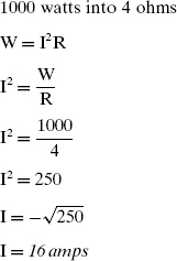
A loudspeaker cable, like an electrical power cable, needs to have a current carrying capacity such that it will not overheat, and a voltage insulation such that it will not arc, but the current carrying capacity of a loudspeaker cable cannot be calculated from the simple W = I2R formula that would apply to the wiring of an electric heater. What is more, loudspeaker cables may be carrying 11 octaves of frequency range and not just the single frequency of an electrical supply, so what happens over the whole range of operation is of interest, and all frequencies must be passed as uniformly as possible.
In the case of the vast majority of transistor amplifiers we are dealing with what amounts to a constant voltage source. This means that from the minimum rated load impedance up to infinity, the output voltage of the amplifier, for any given input voltage and at any frequency within its range, will be independent of the load to which it is connected. However, this is not the case with valve (tube) amplifiers, whose output loads must be critically matched to the output impedance of the valves, usually via a relatively complex output transformer, but for now we will restrict our discussion to the more typical transistor amplifiers.
In order to behave as a voltage source, and remain independent of load, the output impedance of the amplifier needs to be very low indeed – typically hundredths of an ohm. The ratio of the load impedance to the output impedance gives us the damping factor, which is an indication of the ability of the amplifier to suppress the natural resonances within a loudspeaker. This electrical damping effect can be easily tested by lightly tapping the cone of a low frequency loudspeaker with the amplifier connected but turned off, then comparing the sound by tapping again with the amplifier switched on. A significantly deader sound should be heard in the latter case, when the near zero output impedance of the amplifier short circuits the voice coil. A similar effect can be demonstrated without an amplifier, simply by connecting a wire between the loudspeaker terminals, thus short-circuiting the coil.
When a loudspeaker diaphragm is struck, it behaves like a microphone. In fact, when a loudspeaker is connected to a microphone pre-amplifier input it makes quite a good microphone. The movement of the diaphragm in response to vibrations in the air moves the coil within the field of the magnet, which generates a voltage across the terminals. If the terminals are short-circuited, a current flows which tends to drive the voice coil in a direction which opposes the resonant movement of the diaphragm. The shorted coil acts as a dynamic brake. The damping effect of an amplifier can greatly ‘tighten up’ the sound of the bass, because it allows the amplifier to better control the resonant movement of the low frequency drivers. In other words, the transient response is improved. The need for a very good short circuit is important, so if the resistance/impedance of a loudspeaker cable is not close to zero, the damping will not be as close to perfect as possible, and therefore the effect of the amplifier on the loudspeaker resonance will be reduced.
When dealing with such low impedances as are found in typical loudspeaker circuits, such as 4 ohms or less, we are dealing with impedances much lower than would normally be encountered in general electrical wiring. In order to achieve a moderately good damping factor of 40 on a 4 ohm load, the total of the series impedance exhibited by both the amplifier output impedance and the cable impedance could not exceed one tenth of an ohm.
The principal concern of an electrical engineer, when choosing a gauge of cable, is that it will pass the required current without either overheating and producing a fire risk, or causing a voltage drop due to its predominantly resistive impedance (at 50 or 60 Hz) which would reduce the effectiveness of the device to which it is connected. So, if the motor is running at its correct speed and the cable is stone cold, then that is more or less the end of the story from an electrician's point of view.
Conversely, far from dealing with a fixed voltage at a single frequency, a loudspeaker cable has an impedance which may be dominated by its resistance only at low frequencies. At high frequencies the inductance can be contributing more to the impedance than the resistance, and a loudspeaker working on the end of a 10 metre cable producing the same SPL as when connected to the output of the amplifier with 50 cm of cable is no indication that the cable is lossless. If a cable has a resistance of 1 ohm and is connected to an 8 ohm loudspeaker, the voltage drop across the cable would be one part in 9 (i.e. across 1 ohm out of 9 ohms total). This represents about 11%, or about 1 dB, which would be barely audible. For a voice announcement installation, such a cable may be entirely acceptable, but for a high quality music system it would impose a serious limit on the damping factor, and hence on the accuracy of the transient response at low frequencies. The subsequent resonance due to the loss of damping may even restore the 1 dB loss of perceived volume, but the nature of the sound would have changed.
From the point of view of the loudspeaker, the cable is a part of the output impedance of the amplifier, and the damping factor is defined by:
![]()
In other words, the load impedance divided by the output impedance. Therefore, if an 8 ohm load was connected directly to an amplifier having an output impedance (source impedance) of 0.1 ohm, the damping factor would be 8/0.1 or 80. If the two were now connected by a cable having a resistance of 1 ohm, the damping factor would be dependent on the combined resistance of the source and the cable: 1+0 1 ohms. The resulting damping factor would be:
![]()
which in audio engineering terms is poor, and likely to lead to subjectively woolly bass.
At higher frequencies, the drive units which are used do not generally have the mass or compliance to freely resonate, and are additionally resistively damped by the air load. However, at these frequencies the cable inductance can behave like a frequency dependent resistor, and act as a filter. When used with loudspeakers which present variable impedance loads with relation to frequency, both the resistance and the reactive components of the impedance can act as potential dividers, giving rise to a frequency response that varies according to the relative values of cable impedance and loudspeaker input impedance. The loudspeaker response will then vary in different ways as cable length is varied.
Cables also have capacitance between the conductors, but this is not usually problematical because the capacitive reactance is so low compared to the impedances of loudspeaker circuits that its effect would not normally become apparent until hundreds of kilohertz. However, it has been known to affect some marginally stable amplifiers, although it could be said that these problems should be solved at source. Some cables are intentionally capacitive, up to 0.2 microfarads, to maintain the high frequency response at the loudspeaker terminals, but they may unpredictably alter the performance and stability of amplifiers.
6.8.2 The status quo
In terms of professional use, a marginally stable amplifier has little to justify its use. In fact, a marginally stable professional amplifier is almost an oxymoron – a contradiction in itself. However, in the world of hi-fi, some designs exist which are so esoteric that practicality and justifiable engineering are not high on the list of design priorities. Some of these are more works of art than works of science, and they are designed to be pampered and appreciated rather than to be bolted into a rack and forgotten about. Nevertheless, without doubt, some of these specialised hi-fi amplifiers do perform extremely well under the limited circumstances of their intended use, but some are so minimalistic in their design, (even if not in their price) that they can sometimes be only marginally stable (although very few), and often their unbalanced input circuits and high sensitivity (100 mV as opposed to 1 volt) make them more prone to disturbance than the less sensitive and often more robust professional designs. It is therefore not surprising that such amplifiers may show a higher degree of sensitivity to both the input and output cables with which they are connected than do the more robustly designed amplifiers for professional use, which must work even in relatively hostile environments. However, the term ‘professional’ does not ensure sonic transparency, and some supposedly professional amplifiers which are more robust than transparent would not be very sensitive to cable differences due to their own limited performance.
In all fairness, it must be stated that domestic high fidelity and professional recording are two different worlds. Despite the fact that they have a lot in common, they also have many differences. Whilst professionals tend to work with standardised, known, and objectively designed equipment, domestic equipment tends to be individualistic, and marked by diversity more than commonality. Often, in the home of a hi-fi enthusiast, the equipment has pride of place, where aesthetic design can be almost as important as sonic design, and where minimalism and purity at domestic listening levels take precedence over the tolerance of hard-driving and abuse which may be needed by professional equipment. An idiosyncratic, 8 watts per channel valve amplifier has rarely found a home in a professional recording studio, and especially not if it cost 5000 euros or more. It is therefore worth re-emphasising that the innumerable stories about either input or output cables magically changing the sound of domestic equipment (whilst a giant and highly respected organisation such as the BBC has ‘no policy’ on esoteric cables) are more a testament to the sensitivity of much domestic equipment to minor changes in termination than to the general importance of esoteric cable design or materials of construction. However, that is not to say that cables are cables, and that any cable will suffice for connecting a loudspeaker as long as it manages not to catch fire at full volume. So, perhaps we can now look at some of the more important aspects of professional loudspeaker cable design. [Although we should perhaps note, here, that professional recording engineers do tend to be rather more conscious of microphone cable design].
6.8.3 Cable designs for loudspeaker use
The first way to combat the resistance problem is to shorten the cable; halving the length of the cable will halve all the impedance components. Another way to halve the resistance would be to double the cross-section of the cable, but whilst this may be effective on the resistive part of the impedance, the increased spacing between the centres of the conductors will increase the inductance. The effect may therefore be beneficial at low frequencies but detrimental at high frequencies. A way to overcome this problem is to use a co-axial cable, where the two conductors share the same axis. This can minimise the inductance by effectively cancelling the opposing magnetic fields in the two conductors, but as a result of this construction there is more opposing surface area between the conductors, so the capacitance can increase moderately, although this will usually not be a problem. What is important is to always keep the pairs of loudspeaker wires as close and parallel as possible. This enables the magnetic fields around each core to cancel as much as possible of the inductance. Twisting the wires is another way to achieve this, but twisted wires are inevitably slightly longer than straight wires for any given overall length of cable. Well designed twisted cables have proved to be successful in high quality applications. What should be avoided is the use of single wires, each following its own route to the loudspeaker. Such configurations can act as effective aerials, and can introduce RF interference into amplifier circuitry. Figure 6.5 sums up the general philosophy.
There is also a phenomenon known as skin effect. It is a controversial subject as to what effect it has at audio frequencies, but, as was shown in Figure 6.3, if high frequency roll-offs give rise to significant phase shifts below 20 kHz, then their effects may be audible. Skin effect is the tendency for high frequencies to travel through the outer skin of a conductor, and not through the centre of the core. The whole cross-section of the conductor is therefore not used, so the resistance rises as the conducting section of the cable reduces, introducing a high-frequency roll-off. Once again, the shorter the cable, the less the problem.
Some manufactures have opted to address the problem by plating the outside of the conductors with a lower resistance metal. Another approach is to use Litz-wire, where multiple, individually insulated, hair-like wires are twisted together. They thus have a much greater ratio of surface area to volume. The evidence seems to suggest that on lengths of 10 metres or more, this type of cable can exhibit improved results when compared with ‘ordinary’ loudspeaker cables, but in professional situations, placing the amplifiers 10 metres from the loudspeakers would not normally be considered to be good engineering practice, for other reasons which will hopefully become apparent from the latter sections of this chapter. But first let us look at some detailed measurements which were made on loudspeaker cables
6.9 The amplifier/loudspeaker interface
It must be clearly understood that when a loudspeaker is used with an amplifier employing negative feedback from the output stage, either globally or locally, (and at least 99.9% of amplifiers in professional use are so designed) the loudspeaker cable passes signal in both directions. The amplifier sends drive voltages to the loudspeaker, which cause currents to flow through the complex impedances which the loudspeakers present as a load.The reactive components of the impedance, and in particular the moving mass component of the diaphragm/coil assembly, give rise to back-EMFs as the whole assembly resonates in the magnetic field. These EMFs (electro motive forces, or voltages) produced by the resonating loudspeaker acting as an electrical generator rather than as a motor, arrive at the amplifier output terminals via the loudspeaker cables. The circuit of the system is shown in Figure 6.6. The low output impedance of the amplifier cannot effectively damp the back EMFs (reverse voltages) generated by the natural movements of the loudspeaker if an excessive impedance, in the form of a cable, is separating the coil from the output terminals of the amplifier. Cable impedance (or lack of it) is therefore critical in terms of optimising the performance of the amplifier/loudspeaker combinations. It can thus be seen how the cable can control what passes from the amplifier to the loudspeaker, by virtue of the frequency dependent nature of its impedance, and it can also control what passes to the amplifier from the loudspeaker, and hence affect the damping of the transducer system. The effect of any loudspeaker cable therefore must be considered in both directions.
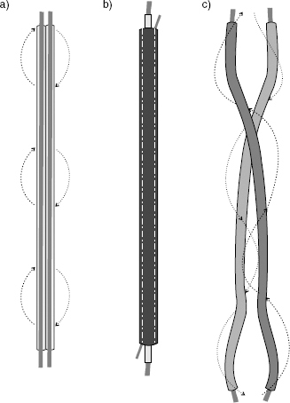
Figure 6.5 Magnetic fields surrounding cables. Better cancellation lowers the inductance.
a) parallel conductors. Partial cancellation as parallel conductors exhibit only weak external magnetic fields – the resulting inductance is low. b) Coaxial pair. Almost total cancellation of the magnetic field due to the concentric conductors – the resulting inductance is very low. c) Unrelated pair. Due to the relatively wide and random spacing of the conductors there is little cancellation of their magnetic fields, so the inductance tends to be higher than for the cables shown in (a) and (b)
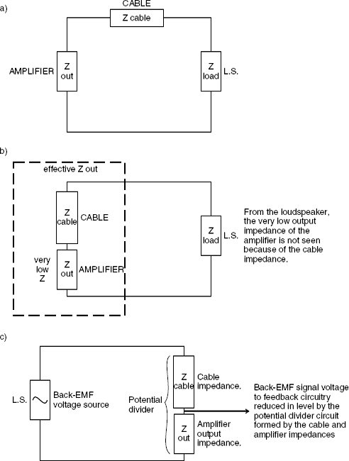
Figure 6.6 Circuit diagram of the amplifier, cable and the loudspeaker impedances. a) Basic circuit. b) Effect on damping. c) Effect on back-emf
One great problem about generalising about many, or most, of the effects of the performance of loudspeaker cables (once the basic properties of resistance and inductance have been adequately specified) is that their effects can be so system-specific. In other words, what occurs with one combination of amplifier, loudspeaker and location may have very little in common with what occurs with a different combination. The only universal solution for minimising the effect of loudspeaker cables is to minimise their length, by mounting the power amplifiers as close as practically possible to the loudspeakers. A total length of about 2 metres from the amplifier terminals to the motor/driver terminals is a reasonable maximum to aim for. And of course, suitable cable must be used. In the experience of the authors, the differences between cables of appropriate resistance and inductance at lengths below 2 metres are too small to be of any real significance, but exactly what section should be used for what power rating of loudspeaker is something that needs to be worked out case by case. For example, as previously mentioned, an excessively large format cable may be detrimental to the response of a tweeter because the increased cable inductance, due to the cable spacing, may be more of a problem than the increased resistance of a thinner cable.
There exist some large, high powered, passively crossed over, professional monitor systems that are very difficult to drive. When the drive voltages going forward meet the back-EMFs coming in the other direction, all in the highly reactive circuitry of a low impedance, passive, high order crossover, peak currents of up to 100 amps have been measured during some complex musical passages at high studio monitoring levels. It would seem obvious that a cable specified for such a system, using amplifiers capable of driving continuously 3000 watts into half an ohm, would need a higher specification than the cables used in a system of similar power rating and acoustic output but using an active crossover, multiple amplifiers, and where the low frequency drivers presented an almost uniform impedance to the amplifier, (at least in the frequency range over which they were being driven).
When calculating the cross-section of loudspeaker cables, we cannot simply take the approach:
As 1 mm2 of cable will safely carry 5 amps, we will therefore use 4 mm2 cable to give a little margin of security.
In terms of electrical engineering, the above concept is a perfectly safe and viable approach, there is no possibility of the cable overheating, but it in no way takes into account the effect on the sonic perception of musical signals when amplifiers are driving difficult loads. In the case of loudspeaker cables, the emphasis is on the cable impedance rather than thermal/current capacity.
6.10 Some provable characteristics of cable performance
In the autumn of 2002, the authors, together with other collaborators, made a presentation to the Reproduced Sound conference of the Institute of Acoustics2. Figures 6.7, 6.8 and 6.9 were taken from that paper. They were from an experiment made at Czerwinski Laboratories in California, by two Russian engineers, Alexander Voishvillo and Alexander Terekhov, accompanied by Eugene Czerwinski, (the founder of Cerwin Vega). [In the 1950s Czerwinski had designed the first of its kind 10,000 watt amplifier using germanium transistors for sonar systems for the US Navy.] They carried out tests on three, 6 metre lengths of different cables, firstly into a resistive 8 ohm load (Figure 6.7), then into a full-range loudspeaker system (Figure 6.8), and finally into a cabinet-mounted low frequency driver (Figure 6.9). The amplifier driving the cables was fed with a multitone test signal3,4, designed to show up non-linear distortions; in particular intermodulation distortion. In Figure 6.7 it can be seen that all six plots are more or less the same. The left hand plots were measured at the amplifier output terminals, whilst the right hand plots were measured at the other end of the 6 metre cables – at the resistive load. The three very different cables all appeared to perform equally. This was what the experimenters were expecting to occur, independently of the load. They were all very much sceptics with regard to significant loudspeaker cable differences – at least between adequately rated cables. However, when they replaced the 8 ohm resistive load with a passively crossed-over loudspeaker system, they were surprised to see the results as shown in Figure 6.8. With the more complex load, all the plots had changed. After changing the load to the low frequency loudspeaker, all the plots changed again, as shown in Figure 6.9. The distortion patterns were noticeably different, not only between the cables, but also between the input and output ends of each cable. The implication here is that the cables change the way that the complex load is seen by the amplifier. Voishvillo reported that upon seeing this, Czerwinski exclaimed “But they're only short cables!”
Figure 6.10, taken from the same IOA paper2, shows six twin plots. In each case the upper trace was the measurement at the amplifier end of the cable, and the lower trace was made at the loudspeaker end. The measurements were taken in a city-centre office with typical city EMI (electromagnetic interference). The input signal was a 1.6 kHz square wave, and the load was a TAD 2001 compression driver, mounted on an axisymmetric horn and producing 70 dB SPL at a distance of one metre. This was intended to represent conditions of realistic use. Plots a) and b) are of 5 metres and 50 metres of RG59 coaxial RF cable, respectively. Plots c) and d) are of a typical, transparent insulation, oxygen-free copper loudspeaker cable, again 5 metres and 50 metres respectively; and plots e) and f) are as a) and b), but with the conductors reversed (i.e. screen to hot and core to ground). Whilst listening only to the background noise from the amplifier, at very low level, no change could be heard between any of the cables, but the potential for such changes in interference patterns, especially on the longer lengths of cable, does not bode well for the inaudibility of these effects on complex musical signals. It was suspected that some amplifier designs could be more susceptible than others to this type of interference entering their feedback circuits via the output terminals. The gross differences in the interference patterns between b) and f), using the selfsame cable but reversing its polarity [hot down the screen in f)] is suggestive of something untoward occurring.
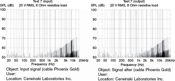
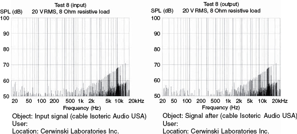
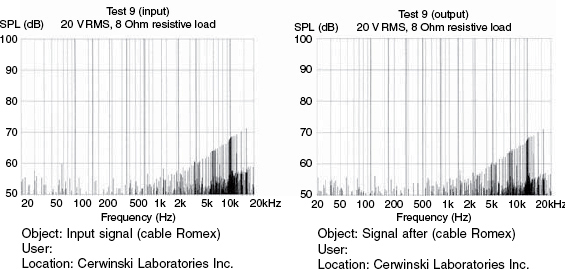
Figure 6.7 Three 6 m cables feeding on 8 ohm resistive load. The left-hand plots are from amplifier output terminals. The right-hand plots were taken from the load
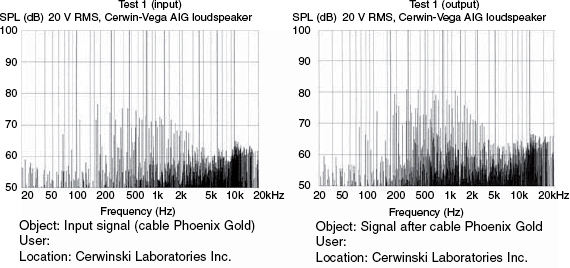
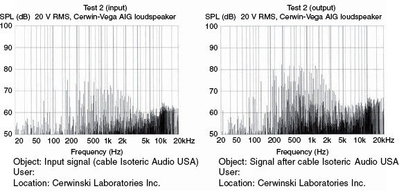
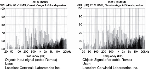
Figure 6.8 Three 6 m cables feeding a full-range loudspeaker with a passive crossover. The left-hand plots are from the amplifier output terminals. The right-hand plots were measurements from the loudspeaker cabinet input terminals
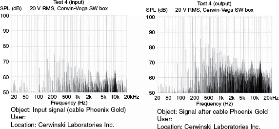
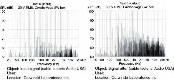
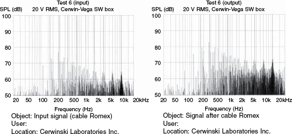
Figure 6.9 Three 6 m cables feeding a sub-woofer box. The left-hand plots are from the amplifier output terminals. The right-hand plots were measurements from the loudspeaker cabinet input terminals
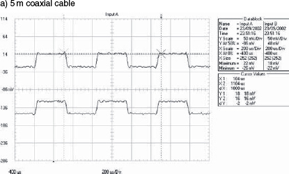
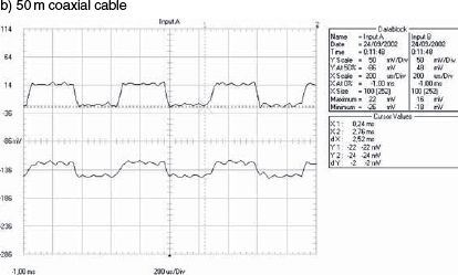

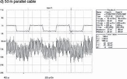
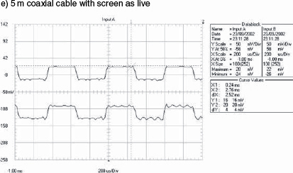
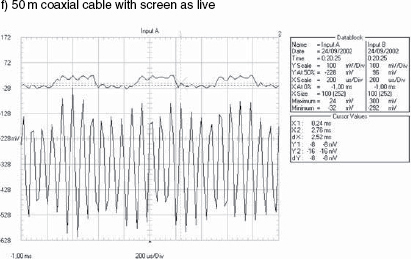
Figure 6.10 Effects of cable on 1.6 kHz square wave. All upper traces are from the amplifier output terminals; all lower traces are from the loudspeaker input terminals
Twelve months later, a further paper was presented, this time to the Reproduced Sound 19 conference, in Oxford5, largely intended to answer questions raised during the previous year's presentation. A series of five tests were undertaken, interchanging the amplifier, cable, and loudspeaker within the same basic tests set up, to see if any changes were noticed in the interference levels. As had been seen the year before, a considerable amount of hash was being received from the air, including a 13 kHz signal which seemed to disappear around 9 pm each evening, even though nothing in the office or workshop was switched off at that time. In the first set up, a high sensitivity compression driver was used as a load, mounted on a horn and producing a 1 kHz tone at 80 dB SPL at one metre. It was driven by a Class A amplifier, designed for professional use and connected via 28 metres of 4mm2 OFC (oxygen-free copper), parallel conductor loudspeaker cable. The results are shown in Figure 6.11. The test was then repeated, but with a dome tweeter of similar frequency response but 20 dB less sensitivity. The amplifier was duly increased in gain to once more produce 80 dB SPL at 1 metre, and the resultant plots are shown in Figure 6.12. Inspection of Figures 6.11 and 6.12 clearly shows how, whilst the absolute interference level has remained almost constant, the extra 20 dB of signal has swamped the noise in the second test. The plots were normalised to the level of the 1 kHz signal level, towards the left hand side of each graph. The frequency scales are linear, not logarithmic. The implication from this is that if the interference pick up could affect the performance of the amplifier, even if it was not directly audible from the loudspeakers, then the effect would be more noticeable on higher sensitivity drivers than on lower sensitivity drivers.
This was an interesting finding, even though it was not definitive, because the motivation to do the investigations leading to the 2002 paper4 came after the usual OFC loudspeaker cables were changed to RG59 coaxial cables between the amplifier and compression drivers in a large studio monitoring system. Many people noticed the difference, even though no difference could be measured in the acoustic output. People (professionals) reported the sound as being smoother with the coaxial cable. The studio in question was sited close to emergency service aerials (fire and police) yet nobody had commented about similar problems in similar monitor systems in other locations. The original complaints of an unusual slight harshness in the sound only applied to the high sensitivity loudspeakers, and not to any other loudspeakers in the studio. The change to the RG59 solved the problem.
The next test in the series was a repeat of the test whose results were shown in Figure 6.11, except that the parallel conductor, 4 mm2 OFC cable was replaced by a 2.5mm2 coaxial loudspeaker cable (not a co-axial RF cable, as used in Figure 6.10). The results are shown in Figure 6.13, which, when compared with Figure 6.11 show much less interference at the loudspeaker end (which may, or may not, be consequential) but a greater level of the 13 kHz interference at the amplifier end of the cable. The voltage sensitivity of the measurement scales is approximately equal in each case.
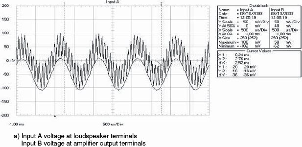
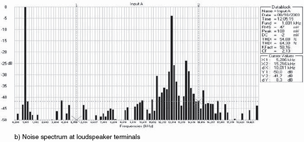
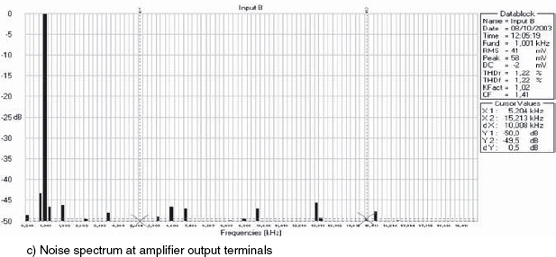
Figure 6.11 Class A amplifier/parallel cable/compression driver
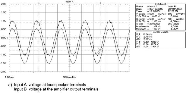
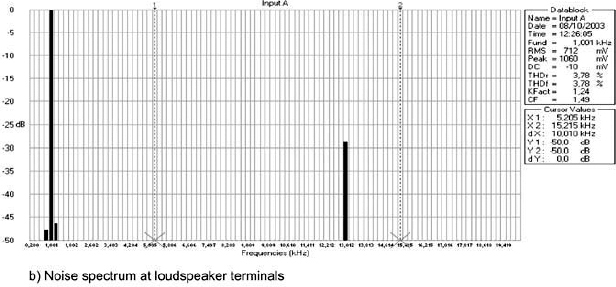
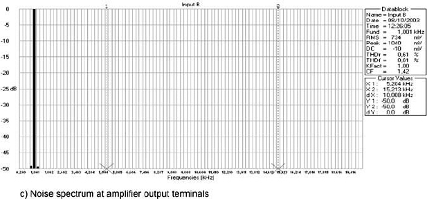
Figure 6.12 Class A amplifier/parallel cable/dome tweeter
The fourth measurement in the series used the same loudspeaker and cable as in the previous measurement, but the Class A amplifier was substituted for a Class AB amplifier. The amplifiers differed considerably in their quantity and application of negative feedback. The results of this test, shown in Figure 6.14, differ greatly from those shown in Figure 6.13. Repeating the last test with parallel cable in place of coaxial cable gave the results as shown in Figure 6.15. In the paper it was stated “Comparison [of the plots in the figures] shows that the interference signal measured at the loudspeaker driver terminals is affected differently by each amplifier, and that the difference in the interference patterns from cable to cable is also influenced by the amplifiers to which they are connected. Given the obvious interdependence of all the parts of the circuit, the findings help to explain why such a lack of consistency exists between reports of the beneficial effects of using certain loudspeaker cables. It would appear to be the case that certain cable benefits can only be claimed for certain amplifier/loudspeaker combinations, and that any perceived audible improvement heard on any one combination may not necessarily be able to be expected when the cable is used on any other combination”.
Perhaps it is also worth looking at some other findings from the same paper, which attempted to measure the losses actually occurring within different cables of different construction and with different loads. Figure 6.16 shows the results of some measurements made by connecting the two inputs of a differential amplifier across the amplifier and loudspeaker ends of some two-metre sections of cable5. The rise in the plots above 2 kHz is a result of the less effective rejection at higher frequencies, so the graphs are comparative rather than absolute: the decibel (vertical) scale is not calibrated. Nevertheless, the differences are real enough. Figure 6.16(a) shows the plot resulting from the measurement of a 2.5mm2, screened, twin twisted-conductor loudspeaker cable. Figure 6.16(b) shows the results for a cat-5 data cable, and Figure 6.16(c) shows the plot for a 6 mm2 twin, parallel conductor loudspeaker cable. All were driving an 8 ohm woofer, but in the latter case, (c), the cone was blocked to prevent any movement. With the cone blocked there is no mechanical resonance, so the dip at around 80 Hz in the first two cases is absent in the case of Figure 6.16(c). The plots clearly show how the losses within different cables are quite different, and how the changes in impedance at the loudspeaker end can further affect the losses in the cables. All the measurements of Figure 6.16 were on lengths of only two metres of cable. Despite the fact that the scaling of the amplitude is only relative, it can still be seen that differences in the losses do exist, not only in terms of overall level but also in frequency balance.
As the evidence presented in this chapter has shown, loudspeaker cables seem to be sensitive to the equipment to which they are connected, and vice versa. What is more, the entire systems seem to be sensitive to their environment, at least in electromagnetic terms. Nevertheless, the concept of minimising loudspeaker cable lengths seems to be well founded, but the practice of separating the frequency range into narrower bandwidths also seems to reduce the demands made of the amplifiers and cables, alike. This is a concept which it is now worth looking at in a little more detail, before expanding the concept to polyamplification and multiamplificaiton.
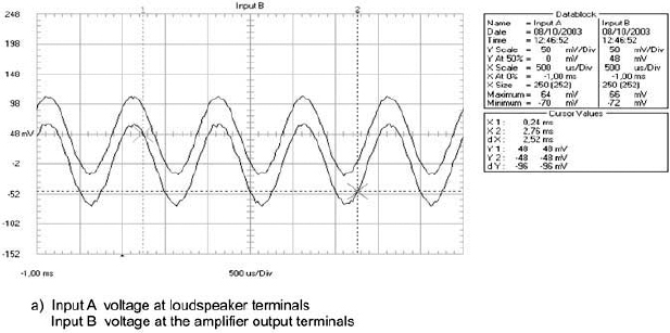
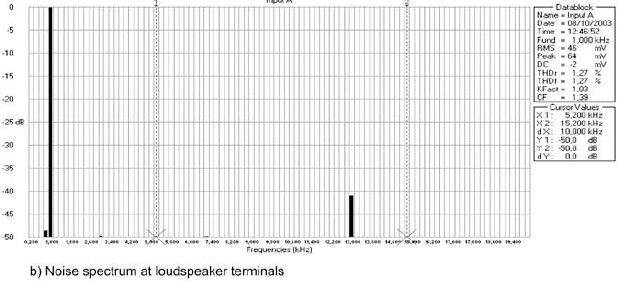
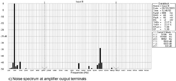
Figure 6.13 Class A amplifier/coaxial cable/compression driver
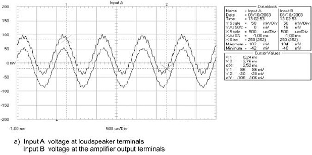
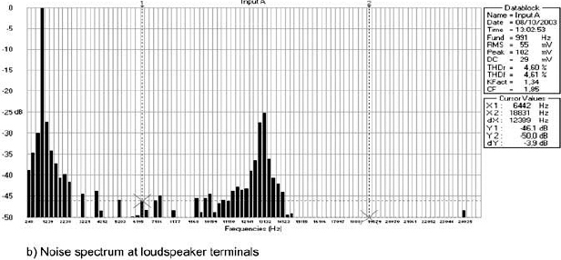
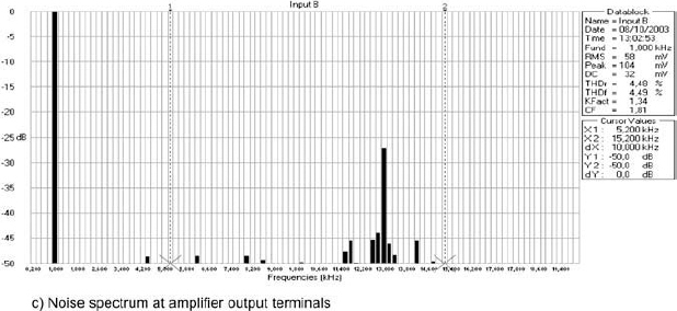
Figure 6.14 Class AB amplifier/coaxial cable/compression driver
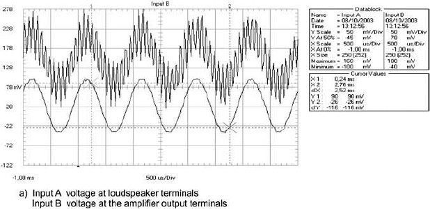
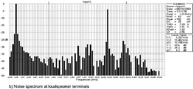
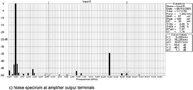
Figure 6.15 Class AB amplifier/parallel cable/compression driver
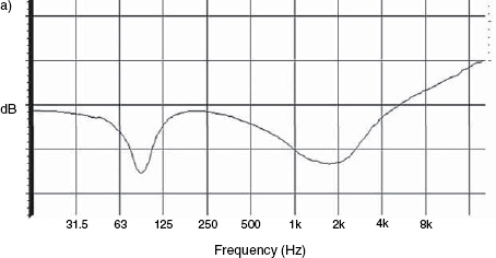
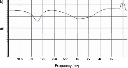
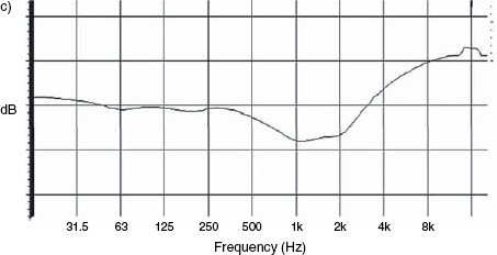
Figure 6.16 a) Spectrum of the difference between the voltage signals at either end of a 2.5mm2 screened cable. b) Spectrum of the difference between the voltage at either end of a CAT5 data cable. c) Spectrum of the difference between the voltage at either end of a figure-of-eight cable with the cone of the low frequency loudspeaker blocked (i.e. prevented from moving). Vertical scale not calibrated
6.11 Some passing comments
Unfortunately for people who have not had a very great degree of experience of the subject, sorting out what is solid from what is nebulous in terms of so much that has been published in the hi-fi press about loudspeaker cables is not an easy task. Nevertheless, despite some critics claiming that it is all a load of nonsense, it is the opinion of the authors that far too many people of good repute have claimed that sonic differences do exist to be able to dismiss the subject of loudspeaker cables out of hand. One of the main obstacles to verification has been the cost of double-blind, controlled tests, with sufficiently large groups of subjects, coupled with the extraordinarily large number of possible equipment combinations and test locations, and the fact that a cable which shows benefits in one of those combinations may show no benefit in another. One component in isolation may not exhibit any noticeable difference over another component. However, when they are used in some combinations with other components, the differences may be readily apparent.
Whilst writing this book, a short, written note was received from Martin Colloms, an eminent authority on the subject of high fidelity loudspeakers. There is nothing to suggest, from either his professional conference papers or his well-respected text books, that he is either cloth-eared or a charlatan, and neither can the authors of this book refute his opinions. An extract from his communication will serve as a good summary.
A fair percentage of my reviewing life has been spent listening to and dealing with cables. Most evaluations I still do blind. I think that I have correlated with reasonable precision the key aspects of cable design from some 400 examples.
Metallurgy: the actual metal or alloy and its state/annealed/crystalline composition/extrusion direction and subsequent build orientation.
Dielectrics alter the sound, as do different plastics in film capacitors, the issues including dielectric factors, DF with frequency, piezo effects, self-damping including semiconducting insulation, and dielectric constant.
Geometry: spacing, stranding, Litz or bunched.
Mechanico-acoustic: physical strength, rigidity, self-damping, microphony issues.
RFI: can be very important; if you spectrum analyse (I work up to 1.5 GHz) the dominant RFI (radio frequency interference) is about 1 MHz for many loudspeaker cables.
Many amplifiers are no longer anything you would recognise by 100 kHz, never mind the 1 MHz, and the RF gets in the output terminals and intermodulates around the feedback loop. A speaker cable is often a good medium-wave aerial.
Cables vary greatly in how they dump RF interference into the amplifier output port. The Zobel filter has little effect as it is generally buffered by 10 ohms. If the RFI doesn't get in the positive line, it common modes into the ground line.
At 1 MHz or more, the RFI hardly cares what kind of amplifier it is. Contacts and connectors also matter, as do their tightness and vibration resistance. Acoustic energy ends up being mechanical watts and everything shakes about.
It is amazing how mild that vibration can be and still affect the sound of an electrical component, including a cable. Simple tests on vibration isolation and suppression show this clearly. Acoustic/mechanical coupling remains one of the most insidious modes of sound quality loss.
In a recent conversation, Paul Frindle, one of the designers of the Sony Oxford R3 digital mixing console and many of the Sony professional plugins, recalled an occurrence during his time as a designer at Solid State Logic. There had been complaints from many studios around the world that mixes done on the small faders, which were simple potentiometers, sounded better than mixes done on the large faders, which operated VCAs (voltage-controlled amplifiers). They proceeded to make countless measurements at the factory but could find no apparent cause for the described difference in the sound. Some of Paul's comments were very reminiscent of loudspeaker cable anomalies.
P.F. “You could end up in a situation where a single signal sounded fine, but its relationship with everything else was ill-defined. You could set up a mix on the pots (the small faders), with no VCAs, and it would sound great; but going through the main faders, with the VCAs, it would sound oddly wrong. Yet, if you soloed any single VCA channel you could hear no difference compared to the small fader. It was fascinating! I found that this was caused by very small amounts of signal dependent delay variance through the VCAs, which was a complex kind of distortion that was unfamiliar within the design context. In my opinion this was one reason that led to the perception that the VCAs sounded bad, and many people went in the direction of consoles with motor driven faders instead.
This problem has some similarity to issues resulting from analogue to digital converters. For instance, if you have different clock-jitter, between channels – this is a lovely one! If your system has timing errors, when you use an ADC and a DAC back to back in a monitoring capacity, the clock is common and simultaneous to both the encoding and decoding stages. Since the timing errors are synchronous they partially null out. However, if you delay the signal – or store it then play it back later – even though the system is the same, the jitter is no longer synchronous, and the resulting sound quality is compromised. In fact, the sound is reminiscent of the mixes done via the VCAs on the old SSL consoles. Of course, this is one of many good illustrations of how the sound can change through a system, even though the recorded bits are unaffected and no numerical errors have actually occurred.
Another similar problem can exist when you dither signals, because of relative correlation. When you dither a number of channels, the dither noise of any one channel should be unrelated and uncorrelated to any other, or you risk the relative correlation of the dither noise starting to become evident. You can end up with statistically partially ‘mono’ dither-noise, which can close in the stereo effect, especially on fade-outs. Again, a single channel works fine, a stereo channel apparently sounds fine whilst the music is playing, but as channels build up with the same dither, the stereo begins to close in. We spent a fortune on the R3 finding 256 independent noise sources, because it was a strange problem to solve. It is hard to measure, and the sound problems are something which you often need to be working on day after day before they become clearly apparent. You feel a sort of unease, that something is wrong, but you can't quite explain what it is. At one time, before we found an easier solution, 30% of the processor of the R3 was dealing with this problem. [And the R3 had about 3000 times the processing power of a current (2005) Pro Tools system. P.N.]
The illusiveness of these types of problems are not dissimilar to the illusiveness of definitive, irrefutable evidence about the differences between loudspeaker cables, but whereas Sony and Solid Stage Logic have been able to throw vast amounts of money at the problems, low volume producers of special loudspeaker cables have not enjoyed such luxury. Two of Paul Frindle's sentences in the previous paragraph are very relevant to the issue. “It is hard to measure, and the sound problems are something which you often need to be working on day after day before they become clearly apparent. You feel a sort of unease, that something is wrong, but you can't quite explain what it is”. There are the hardnosed objectivists who would say that if you cannot measure it, then it cannot be important, but, once Solid State Logic solved their VCA problem, the complaints stopped from the users around the world. Surely this is evidence that the problem had been real enough. There is no logic in claiming that if Paul and his colleagues had not found the problem, then that would have proved that the problem was imaginary. Similarly, if people cannot prove the reasons why cables should sound different, the implication is that not enough effort has been put into finding the problem, and not that the problem does not exist. And, of course, a subtle difference in the sound, given rise to by two loudspeaker cables, will almost certainly not be audible if the resolution of the loudspeakers being used to audition them is not, in itself, high enough to show up the difference.
Nevertheless, the evidence is now overwhelming that cables can give rise to sonic differences. The situation is somewhat paralleled by the relationship between stress and the functioning of the human immune system. Believe it or not, despite the fact that most people ‘know’ that when people are stressed they seem to be more prone to illness and infection, no clinically proven, scientific evidence currently exists to make a definite link between stress and susceptibility to illness. However, in 2002, Ronald Glaser, et al, at Ohio State University, published in the Journal of Consulting and Clinical Psychology a paper stating that whilst no proof existed, the circumstantial evidence was too overwhelming to be ignored. The conclusion was that stress did lead to more illness and infection, and that the fact that they could not prove how it could do so did not mean that it could not be said that it did do so.
6.12 Multi-cabling
It is widely accepted that bi-wiring with conventional loudspeaker cable will almost universally impart a greater sonic improvement to any multi-way loudspeaker system than a change from a single conventional cable to a single esoteric cable. Bi-wiring takes separate cables from the output terminals of the amplifier to the separated inputs of the high and low frequency sections of the passive crossover filters. Figure 6.17 shows the principles of bi-wiring. Tri-wiring simply extends the concept to three filter sections and three cables. Although each cable still receives the same voltage drive from the amplifier, the current passed by each cable is only that which relates to the frequency band that it is handling. As it is the current which gives rise to the linear and non-linear processes which are attributed to magnetic effects, the separation of the currents into two or more frequency bands can be beneficial. The high frequency signals are therefore unaffected by the heavy low frequency currents.
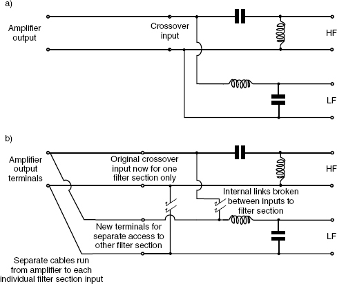
Figure 6.17 a) Conventional amplifier-to-crossover wiring. b) Bi-wiring
The materials used for the conductors can influence the sound quality performance of loudspeaker cables, as can the materials used for the insulators. The physical construction of a cable is also considered by many to be a significant factor in terms of sound quality, with some complex plaiting arrangements of the conductors being highly regarded by many specialists. Given these differences, appropriate cable designs and dimensions can be more ideally matched to the frequency and current requirements of the individual drivers in a system if multi-cabling is employed.
6.13 Polyamplification and multiamplification
What has just been discussed is the way in which the separation of the audio spectrum into different frequency bands can make much fewer demands on the loudspeaker cables, and that in separating the bands, intermodulation distortion can be reduced. This idea can be extended one step further by using separate amplifiers, as well as separate cables, a practice known as polyamplification as shown in Figure 6.18. However, once one has progressed to this stage, there can be little justification in using high level, passive filters when low level, active filters could do the job in a more precise and less lossy way, although the design of audiophile-standard active filters is not an easy task. Nonetheless, the polyamplification system has seen use, and the amplifiers, like the cables in the previous case, are driven by the full, composite signal voltage, although they only need to supply current over their specific frequency bands, reducing intermodulation distortion to a greater degree than bi-wiring or tri-wiring alone.
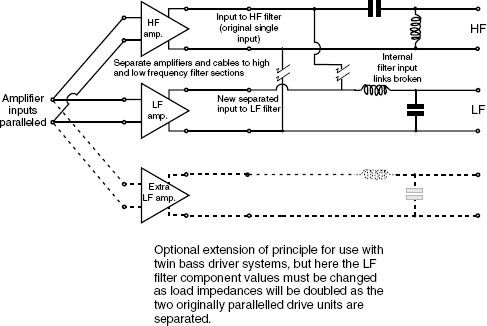
Figure 6.18 Extension of bi-wiring to bi-amplification whilst still using passive, high-level filters
When the filters are placed ahead of the amplifiers, and the amplifier outputs are connected directly to the loudspeaker drive units, with no components other than the cable between them, the practice is known as multi-amplification. Multi-wiring (bi-wiring, tri-wiring etc), polyamplification and multiamplification are three distinct steps forward, respectively, in terms of sonic quality, and it usually does not require trained ears to notice the benefits.
There is no doubt that it is asking a lot of any amplifier, or loudspeaker cable, to faithfully pass up to 11 octaves of musical signal with a dynamic range of 90 dB or more. Considering the fact that no loudspeaker driver can do this, it seems perfectly reasonable to split the frequency bands ahead of the amplifiers and drive each frequency range independently. The benefits of doing this were amply described in Chapter 5, but further repercussions of this practice on amplifiers and cables can be expanded on, here.
It does not take too much imagination to realise how a 20 or 30 amp low frequency current can modulate high frequency signals passing along the same cable at levels of 40 dB below. The bass currents cause the conductors to flex, mechanically, under the mutual magnetic field. Piezo and structural modulation then carries interference into the low level high frequency system. In terms of power ratios, say between tympani and triangles, or bass guitar and mandolin, that 40 dB represents 10,000:1, or a current ratio of 100:1. The more that the frequency bands are separated, the easier they are to handle, as with the drive units themselves. It has been the experience of the authors that as the frequency bands become narrower, the need for specially selected cables reduces considerably. The Litz wire referred to in Section 6.8 may be beneficial when used in 10 metre lengths and handling the full audio frequency range, but those benefits when used in 2 metre lengths when handling only frequencies below 1 kHz would be minimal.
In a similar way, the separation of the different frequency bands can allow the selection of amplifiers which are less heavy, expensive, heat producing or physically large, without significantly compromising performance. What is more, if any non-linearity exists in the circuitry, which it must to some degree, the potential for the production of intermodulation distortion will be greatly reduced. The potential for the low frequencies to modulate the more delicate high frequencies will not occur, and, as discussed in Chapter 5, the generally prevailing opinion is that multi-amplified systems sound ‘cleaner’ than equivalent systems using single, full-range amplifiers. And of course, with multiamplification, multi-cabling is an automatic result.
6.14 System design
Before selecting amplifiers or cables for any loudspeaker system, it is necessary to have a clear view of the purposes for which the entire system will be used. There simply does not exist any ideal amplifier or ideal cable to serve for all purposes. One cable which improves the sonic quality of given combinations of amplifier and loudspeaker may show absolutely no benefit whatsoever with a different combination. One amplifier which sounds stressed at high levels when driving a loudspeaker exhibiting a ‘difficult’ input impedance may perform excellently in combination with a loudspeaker with a more uniform impedance curve.
Perhaps nothing highlights the concept of component matching quite so easily as carefully listening to the performance of digital-to-analogue converters (DACs). The subtle, or even not-so-subtle, differences between better quality DACs will be revealed by a high resolution monitor system in a good listening room. However, it is possible to substitute loudspeakers of progressively lesser quality of reproduction, and to continue to repeat the tests until no difference can be heard between the different DACs. To a lesser degree, the same effect may be noticed when changing amplifiers or loudspeaker cables. When considering the components for a system it is not usually considered to be commercially viable to over-specify any component part. For this reason, in general, an amplifier will be used in a powered loudspeaker which is ‘only’ of a quality up to which it is deemed that no further improvements in amplifier performance would give rise to any significantly noticeable improvement in the sound of the complete system. Even in professional systems, it is rare in the 21st century for manufacturers to over specify anything. However, in terms of professional engineering, as opposed to engineering for the market, it can still be beneficial to design systems with an extra margin of quality to allow for minor deterioration over time, or to allow for minor degradations elsewhere in the chain. A 1000 euro, star quad, polarised, screened cable may possibly make a difference in geographical areas of high electromagnetic interference, and when used with amplifiers which are sensitive to having long ‘aerials’ hung on to their outputs, but there would be no justification using the same cable in interference-free areas with amplifiers which were immune to the problem.
What equipment is truly professional and what is not can be difficult for many inexperienced people to decide in days when marketing is so aggressive, and when ‘professional’ is a word often used more as a sales device than an accurate representation. In fact, as so much recording is carried out in places which could hardly be described as professional in the traditional sense, and yet which do much work commercially, the whole line between professional and domestic equipment has become very ill-defined.
References
1 Newell, P. R., ‘Studio Monitoring Design’, Chapter 6, Focal Press, Oxford, UK (1995)
2 Newell. P., Castro, C., Ruiz, M., Holland, K., Newell. J., ‘The Effect of Various Types of Cables on the Performance of High Frequency Loudspeakers’, Proceedings of the Institute of Acoustics, Vol 24, Part 8, Reproduced Sound 18 conference, Stratford-upon-Avon, UK (Nov 2002)
3 Czerwinski, E., Voishvillo, A., Alexandrov, A., Terekhov, A., ‘Multitone Testing of Sound System Components – Some Results and Conclusions, Part 1: History and Theory’, Journal of the Audio Engineering Society, Vol 49, No 11, pp 1011 – 1048 (Nov 2001)
4 Czerwinski, E., Voishvillo, A., Alexandrov, A., Terekhov, A., ‘Multitone Testing of Sound System Components – Some Results and Conclusions, Part 2: Modeling and Application, Journal of the Audio Engineering Society, Vol 49, No 12, pp 1181 – 1192 (Dec 2001)
5 Castro. S.V., Newell, J. P., Ruiz, M., Holland, K. R., Newell, P. R., ‘Loudspeaker Cables for High Frequency Transducers – A Further Assessment’, Proceedings of the Institute of Acoustics, Vol 24, Part 8, Reproduced Sound 19 conference, Oxford, UK (Nov 2003)
Bibliography
1 Duncan, B., ‘High Performance Audio Power Amplifiers’, Newnes, Oxford, UK (1996 – Reprinted with revisions 1997)
2 Newell, P. R., ‘Studio Monitoring Design’, Focal Press, Oxford, UK (1995)
3 Newell, P. R., ‘Recording Studio Design’, Focal Press, Oxford, UK (2003)
4 Harris, S., ‘Class D Audio Power Amplifiers’ Audio Engineering Society, 18th UK Conference Proceedings, London (2003)
5 Colloms, M., ‘High Performance Loudspeakers’, 6th Edition, John Wiley & Sons, Chichester, UK (2005)