
Chapter 8
Form follows function
8.1 The chain
The recording chain under discussion here begins with the musicians and ends in the rooms in which the people who buy the recordings choose to place their music systems. Domestically, we must really limit this discussion to reasonably high fidelity systems, because once we introduce in-car listening and ghetto-blasters on the kitchen table, or portable radios in the bathroom, we begin to enter a realm of variability which, firstly, become unable to be qualified and secondly, in the majority of cases, cannot really be considered capable of truly representing the music producers’ wishes. Manufacturers of such equipment may go to great lengths to produce pleasant-sounding equipment, and record producers may go to equally great lengths to ensure the compatibility of their mixes with such systems because they represent the majority of the market for recorded music, but this book is essentially dealing with the concept of high fidelity reproduction. This is not to say that many in-car systems are not capable of remarkably high fidelity in many aspects of their performance, but their reproduction quality is still idiosyncratic in a way that generally sets it apart from what we expect to hear from a ‘high-end’ system in the home.
The loudspeakers used in the recording chain can be separated into five basic groups:
1) loudspeakers for musical instrument amplification
2) recording monitors
3) mixing monitors
4) mastering monitors
5) domestic high fidelity loudspeakers
There are many people who will argue against this concept, citing that a good, professional, well conceived, well-engineered loudspeaker should be suitable for all of the above purposes. However, the recording chain is a very varied chain, and what will be discussed in this chapter are the specific requirements at each stage of the process which tilt certain designs or concepts towards being advantageous for the different needs of those specific requirements. In fact, the reality of the current situation is that different loudspeakers do tend to be used in different stages of the recording/mixing/mastering process where financial restraints do not limit the choice of equipment, and there are many good reasons why this state of affairs exists.
In their own ways, the last four of the loudspeakers on the above list all try to achieve the closest approach to the original sound. They are all reproducers, trying to emulate as accurately as possible within their design criteria a faithful acoustical output of the electrical waveform being fed to them. All of them will generally be required to show a wide, flat frequency response, a well-damped time response, low levels of non-linear distortion and a directivity pattern appropriate to the rooms in which they are each expected to be used. The balance of priorities will vary with the intended applications, as we will discuss later, but the above characteristics are common to all of them.
Conversely, loudspeakers for use with musical instruments are part of the instruments which they are amplifying. They are sound producers, not reproducers, and what they produce is, in itself, definitive. They are unlikely to have flat frequency responses, and the range of those responses may well be defined by the harmonic range of the instruments with which they will be used. Colouration of the sound is usually a desirable asset – something which is anathema to hi-fi or monitoring – and ‘musical’ forms of distortion may also be considered to be beneficial. Time responses which contain resonances can impart warmth and character to the musical timbre, and directivity control may be something which is given very little consideration whatsoever. In fact, the design of loudspeakers for the production or reproduction of music have very little in common. Music reproduced via musical instrument loudspeakers may be very far from what the record producers intended, and electric instruments played via high fidelity loudspeakers may tend to sound lifeless and uninspiring.
It may be more appropriate to begin this chapter by looking at the reproducers before discussing the producers, because the idiosyncrasies of the latter will be better understood after the rigours of the reproduction of music have been better appreciated. Nevertheless, there is no hierarchy of superiority in the concepts, because unless an interesting sound is there to be recorded, there cannot be much enjoyment from reproducing it. Indeed, the factories which produce the better musical instrument loudspeakers spend just as much time and attention on the design, manufacture and quality control of the instrument loudspeakers as they do on the best monitoring loudspeakers. In some ways, designing for flatness and low distortion can be easier than trying to design something to make that elusive, ‘magic’ sound.
8.2 Recording monitors
Until the early 1970s, recording monitors, mixing monitors and mastering monitors – in those days, mastering being essentially disc cutting – were largely one and the same thing. It was not uncommon for the same type of loudspeakers to be used throughout the principal rooms of a recording studio complex, although in the disc cutting rooms, which were usually smaller in size than the recording control rooms, the sound was rarely the same as in the usually better acoustics of the control rooms and mixing rooms. In those days, also, the musicians tended to stay in the recording rooms, and only ventured into the control rooms when invited to hear a ‘playback’.
As time progressed, and the musicians began to become more involved in the whole process, they began to spend much more time in the control rooms, and they began to expect to feel the same sensations as they ventured from the performing studios to the control rooms, in order not to lose the ‘vibe’. Volume levels in the control rooms began to rise in order to avoid the deflationary sensation of playing in the studio at 100 dB SPL then listening to the ‘take’ in the control room at 85 dB SPL. If the levels changed, the perception changed, and with it the ‘buzz’ of excitement could change, leaving the musicians in doubt about whether they had achieved their aims, or not. Within a very few years, and especially after the advent of synthesisers and other portable keyboard instruments, it began to become commonplace to actually perform in the control room.
It can be argued that if what is perceived at 100 dB will not translate to 85 dB or less, then there is an inconsistency that suggests that the recording may disappoint when reproduced domestically. However, it should be well understood that, at least for multitrack recordings, the recording phase is about capturing a performance. The experience of the recording staff will be important in deciding if the sounds can be optimised at lower levels, but the achievement of the maximum impact of the performance can only effectively be captured during the recordings.
Around 100 dB SPL, music begins to affect perception and emotions in a different way to what we perceive at lower levels. Chemical changes take place in the brain, which are not unlike those caused by sex and certain drugs. This explains why music at discothèques needs to be loud, or the sensation to dance will not be stimulated and the tendency towards exhibitionism will not be aroused. The exhibitionist tendency is also important in the recording process, because musicians are performers, and a performance is an exhibition. Therefore, if musicians are to perform at their best, they may well need a stimulus, very similar to the disco dancers needing a stimulus. Obviously, the type of stimulus depends on musical style, but under almost all circumstances, the correct stimulus will not be achieved unless the musicians are performing in a control room at reasonably similar levels of sound pressure to those which they would normally be receiving during a concert performance.
Perhaps coincidentally, the tendency to perform in control rooms began around the same time that some ‘mini-PA systems’ were beginning to appear as studio monitors, which could easily produce over 120 dB SPL at the mixing console. In all fairness, much more is known about psychoacoustics in 2005 than was known in 1975. However, in those early days, the mini-PA system with a pair of high power 15 inch drivers, a compression driver straight from sound reinforcement technology on a barely modified horn, and a high power compression tweeter seemed to be a reasonable means to achieve the sort of high SPL, wide bandwidth, relatively low distortion sound that was being called for. Two such systems are shown in Figure 8.1, and even at low SPLs the performance of these systems was better than many of the previously used monitors, at least for many types of music, but they did have many design faults by modern standards. Time has refined these concepts, and room acoustics have taken great steps forward, guided by a much greater understanding of psychoacoustics, but in the conditions of the mid 1970s the failings of the loudspeaker/room combinations in many cases led to problems when using these main monitors for mixing, which in turn led to the use of small reference loudspeakers such as the Auratones, and later the Yamaha NS10s, to name two popular examples. The concept of separate recording and mixing monitors had thus begun to establish itself, and it began to become clear that each had their place in the music recording process. Nonetheless, whilst it is by no means obligatory to use different monitors at the recording and mixing stages, it tends to be rather expensive to achieve conditions with a single system which are optimal for both purposes. Cost-cutting has had a big impact on the limitation of monitoring acoustics to something which is often well below what is achievable.
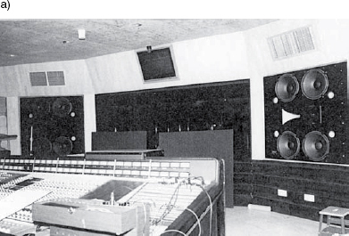
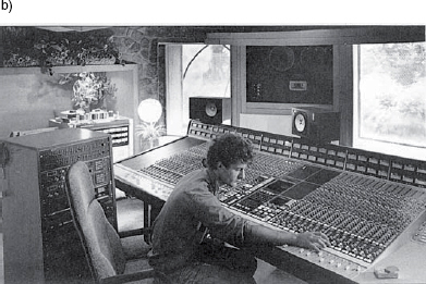
Figure 8.1 Large studio systems from the mid-1980s. a) Giant Eastlake Audio systems at Marcus Music, London, UK. b) Urei 815s at Jacobs ‘Court’ studio, Farnham, UK
8.2.1 Basic requirements
Recording monitors need to do two jobs at the same time. The musicians may be considering them to be stage monitors – performance monitors – whilst the recording engineers will also be using them to assess recording quality and instrumental timbre. They therefore need to simultaneously achieve high SPLs and great subtlety. The musicians will also be expecting them to go as deep as their lowest bass instrument would achieve in a live performance, or their sense of the performance may be diminished. The musicians may also be distributed around the room, and each of them will be expecting to receive their fair share of the sound. The latter fact tends to mean that the loudspeakers need to insonify the entire room to a reasonably equal degree. If this is to be achieved in a way in which the recording engineer can still hear all the necessary detail in the sound, the room will need to be extremely well controlled acoustically, and the loudspeakers would need to be flush-mounted in the wall. Not surprisingly, these are precisely the conditions which are to be found in most of the control rooms of the world's most famous studios. Some rooms complying with these requirements are shown in Figure 8.2.
A typical frequency response requirement is shown in Figure 8.3. The low frequency response needs to go to around an octave below the lowest note on a conventional bass guitar, at 41 Hz. The extra octave is needed both to minimise colouration due to phase shifts associated with the roll-off, which can extend well above the roll-off turnover frequency, and also to accommodate instruments such as the less common five-string bass guitars, and the sub-bass from synthesisers. The perceived colouration due to the roll-off at around 20 Hz is considerably less in this lowest octave of the audio frequency range.
The roll-off at the high frequency end of the spectrum is something which has developed over time. In the early to mid 1970s, when the recording monitors were also the mixing monitors, it was customary to use multi-band equalisers to achieve a flat response up to 20 kHz. However, it soon became apparent that this was leading to dull mixes in the homes of the record buyers. There were several schools of though about why this should be so. One idea was that the higher monitoring levels in the studios meant that the mixes were being done at levels where the ear was more sensitive to high treble than would be perceived at the levels of typical domestic reproduction. Consequently, what would seem to be a balanced frequency response in the studio would seem top-light in the home. Another reason frequently discussed was that the ‘bass trapping’ which was employed in many control rooms, to flatten the low frequency response of the rooms, was not a part of most domestic constructions. Therefore, the increased bass build-up in many domestic living rooms required a corresponding treble boost if a balanced low/high frequency relationship was to be achieved. Nevertheless, whatever the reasons actually were, the treble roll-off became a normal alignment for the large monitors, and it seemed to lead to better results. Nowadays, even if the large monitors are not used so frequently for mixing, the generally higher SPLs at which they are used seems to be less fatiguing with the roll-off of the high frequencies, and a more natural, representative balance is perceived. A rather similar process occurred in the film industry, where an empirically derived ‘X-curve’, with a significant high frequency roll-off, became the industry standard, because it works!
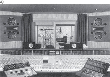
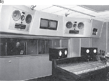
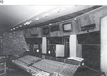
Figure 8.2 a) Kinoshita monitor system at Capri Digital, Capri, Italy. b) Blackwing, London, UK, with its unusual Yamaha NS40 close-field monitors and a pair of 4-way amplified Reflexion Arts 235 monitors, mounted above the soffit. c) Eurosonic, Madrid, Spain
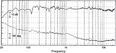
Figure 8.3 Two-way monitor measured on-axis at 2 metres distance in a control room at LMH
By the same token, it would be reasonable to expect that the low frequencies should also be rolled-off. The curves of equal loudness are shown in Figure 8.4, and from them it can be seen that the ear becomes much more sensitive to the low frequency as the level increases. Nevertheless, as we have just discussed, in many domestic rooms the bass is much less controlled than in the most recording studio control rooms, so it would seem to be reasonable that the low frequency increase due to the listening level in the control rooms will very often be matched by the bass build-up in domestic rooms when listening at 10 to 20 dB less SPL. But whatever the reason, at the recording stage of the process, the performance is paramount. Who wants to hear a great recording of a poor performance? The frequency response target of Figure 8.3 certainly seems to work for recording monitors, and experience has shown that it also works well for mixing in the far-field.
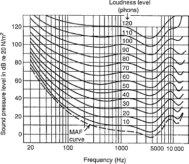
Figure 8.4 The Robinson-Dadson curves of equal loudness
Another important aspect of recording monitors is a fast decay time across the entire frequency band. A typical decay plot is shown in Figure 8.5. A fast decay is important because any resonant overhang will tend to lift the response at the resonant frequencies, just as a resonant mode in a room will cause a lump in the room response close to its antinode(s). The resonances can also mask detail in the sound, as will be discussed in more detail in Chapter 11. Unfortunately, many small monitor systems purposely employ resonances to extend their low frequency responses (see ‘Reflex enclosures’ in Chapter 3), but this technique is bound to blur detail and create the potential for misjudgements about the musical balance between instruments containing mixtures of low frequencies of both transient and steady-state nature, such as the combination of bass drums and bass guitars. Their timbral balance will, to different degrees, be coloured by the resonance, so the recording personnel will be left unsure about which part of the sound is contributed by the recording, and which part is contributed by the loudspeakers and the room. It is therefore important to use physically large monitor loudspeakers because at peak levels of 110 dB SPL at reasonable listening distances, it is simply impossible to achieve fast decaying, low distortion, low frequency responses from small loudspeakers. There is no technology or trickery to overcome this problem because it is deeply rooted in the laws of physics.
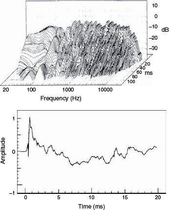
Figure 8.5 In-room decay response of a large monitor system in a well-controlled control room. The resonance evident in the waterfall plot at 120 Hz was the resonance of an empty cable tube in the floor
Mixing is made much easier if the recording stage has been well monitored and controlled. There are far too many cases of problems being heard at the mastering stages due to the mixes having been done on small monitors of recordings which were also done via small loudspeakers, and thus which were not adequately monitored in the first instance. Commercial pressures, and the general decline and de-professionalisation of the recording industry in the late 20th, century has given rise to so many studios which use small monitors for the entire recording process. Many excellent recordings have been made in such studios, partly due to the adaptation of musical styles, such as by using instruments with pre-programmed, well-balanced sounds, and also by the degree of familiarity with the systems which has been developed by the recording personnel. Nevertheless, a whole industry of mastering has since grown to unforeseen levels, partly fed by the uncertainly which many people feel when working in conditions of inadequate monitoring when only small loudspeakers are available.
8.2.2 Proportional costs
Since the 1980s, the cost of multi-track recording systems has plummeted. When inflation is taken into account, the degree to which the prices have fallen is enormous. On the other hand, the price of good recording monitors and excellent acoustics has remained at similar, real, proportionate levels to what they were in the 1980s. That is to say, if a large, stereo monitor system and acoustic treatment cost the same as a new Mercedes car in 1985, then the cost of the same, top-line monitor system and acoustic treatment in 2005 would still cost the same as a new Mercedes car, whereas the price of a recording system has fallen from the price of three entire cars to the price of a replacement engine. Monitor loudspeakers and acoustic control systems are works of engineering, which require skilled labour and careful planning. They do not follow the trend in electronic development at the signal processing level, and micro-miniaturisation and mass production techniques cannot be applied. Even the power amplifiers which are used are physically large devices, which take considerable labour to construct. They also require expensive chassis and bulky components to handle the power levels involved and to dissipate the waste heat. In fact, as time progresses, skilled labour has tended to increase in proportional costs, but mechanisation does not easily lend itself to specialised, low quantity production processes, so high quality amplifier prices also remain high.
This disproportionality in the cost of the recording systems to the monitor systems has strongly militated against the purchase of large recording monitors. In cases where they have been bought, but used in rooms which were not suitably treated for financial reasons, they have often unjustly been criticised for being difficult to use. This however, is down to their inappropriate circumstances of use rather than the failings of the monitor systems, themselves, because such systems cannot be expected to work well in rooms which are not appropriately designed. Much of the criticism which modern, large monitors receive are based on this type of misapplication, although it must be said that some manufacturers have clouded the issue by attempting, for marketing reasons, to make their large monitors mimic the rounder sound of the wider-range smaller monitors. The real job of the large monitors is to do well some things that the small monitors cannot do. Their job is not simply to be a louder version of the small monitors.
8.2.3 Different approaches
Designing a large loudspeaker system to respond in a delicate and subtle manner whilst producing high SPLs is not an easy task. Unfortunately, as the solutions to some problems become easier as size goes up, the solutions to other problems become more difficult to achieve. The diversity in the design of many of the large systems which will now be discussed reflect the different orders of priority which their designers have given to the points where compromises must be made. A loudspeaker system cannot recreate the three-dimensional sound-field produced by an acoustic instrument, but ears are very sensitive to changes in sound-fields. Room acoustics also become more relevant as the loudspeaker to listener distance becomes greater, so the design of the loudspeakers and rooms becomes inextricably linked. The combined sound-field is what the listeners perceive, so if some compromises in loudspeaker system design can be mitigated in their effect by corresponding room acoustic changes, better overall results can be achieved.
The above statement also implies that a loudspeaker system which is designed for one room-acoustic concept may not be appropriate when used in acoustically different rooms, and vice versa. Therefore, to put any large monitor system into a relatively untreated room will be asking for problems – small systems at close distances tend to be a better solution. Nevertheless, a good large system in an appropriate room may be able to achieve a level of overall response accuracy which would simply be unattainable by any monitor system in a poorly treated room, or any small loudspeaker system in any room. However, as previously stated, the option of a large monitor system in an appropriate room is not likely to be a cheap solution to realise.
Figure 8.6 shows four large monitor systems of very high quality, but none of them can achieve their potential without a considerable amount of acoustic design in the control room. And by ‘acoustic design’ we are not referring to sticking some foam panels on the wall. Acoustic control systems which work at 20 or 30 Hz are necessarily large, and their size is dependent upon wavelength, and wavelength alone. They will not scale with room size or budget. This means that rooms with well controlled low frequencies need to be considerably larger than the working space which will be required after the room is finished. Two hundred cubic metres would be a good volume to begin with – a room of around 7 m × 7 m × 4 m high (the fact that it is square may be of no account when the necessary degree of treatment is installed1 – but such spaces are often considered to be uneconomical in the post 2000 recording world. Nonetheless, economics has nothing to do with physics, so the fact remains that in the top professional studios, where things are built to a quality, rather than to a cost, the control rooms tend to be of over 200 m3 in their basic shell sizes.
All the systems shown in Figure 8.6 use multiple bass drivers. The production of low frequencies essentially involves moving a quantity of air which is the product of the moving area and the velocity. In other words, a small radiating area can be moved with a high velocity, or a large radiating area can be moved with a low velocity to achieve the same high SPL. However, the low-velocity, high radiating area approach produces significantly less non-linear distortion. The larger surface area also increases the radiation efficiency, as the large area better matches the characteristic impedance of the air in contact with it. Quite obviously, this cannot be achieved in a small box. The use of multiple low-frequency drivers also mean multiple voice coils, and this tends to lead to better dissipation of the waste heat, so problems of thermal compression are reduced.
Another reason for using multiple drivers as opposed to simply using larger, single drivers is because it tends to become difficult to maintain the rigidity of the piston (the cone) much beyond diameters of 15 inches (380 mm). Beyond 18 inches (460 mm) adequate cone rigidity only tends to be possible by employing means that significantly increase the weight of the moving assembly, which leads to reduced efficiency. Conversely, as the resonant frequency is related to both the weight of the moving system and the stiffness of the suspension, a small, light cone can only achieve low resonance with a very loose, low stiffness suspension. That is, as the weight reduces, the stiffness must also reduce if the resonant frequency is to remain the same. This can lead to excessive fragility for professional use, so cones of less than 12 inches (300 mm) tend not be used in large monitor systems, because they tend to be either inefficient or fragile. Where responses are desired down to 20 or 25 Hz, 15 or 16 inch (380 – 400 mm) drivers seem to be an optimum choice.
The choice of whether to put multiple drivers in the same enclosure or to provide them with individual enclosures is another option. Each of two similar drivers in a 500L enclosure behave theoretically exactly as one loudspeaker in a 250L enclosure. Therefore, whether a cabinet with two drivers has a single 500L volume or is divided into two separate volumes of 250L will in no way affect the theoretical performance of the system. If the loudspeakers are reflex loaded, then obviously the two sections would need their individual tuning ports in a divided enclosure, and the sizes of those ports would be different from the ports needed for the larger, single enclosure. However, if the two enclosures were tuned to the same frequency as the single enclosure, the loading on the drivers would be identical to the case of both drivers being situated in one, larger enclosure.
Well, at least that is the case in theory, but in practice the drivers are rarely, if ever, identical in their performance or resonant frequency. Some designers feel that drivers sharing a single cabinet run the risk of detuning the systems by one driver dominating the port response, but this problem appears to be negligible with large enclosures tuned to very low frequencies. It is a characteristic of more consequence in small, domestic loudspeakers. What is more, as the resonant frequency goes down, the tuning of big boxes tends to become much broader, much less precisely tuned than smaller boxes with higher resonant frequencies. The only real advantage of using separate enclosures for the double woofers in large cabinets is the ability to modify the overall response by using different tuning frequencies for each cabinet, which can be useful in adjusting the response contour to a desired target function.
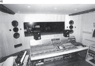
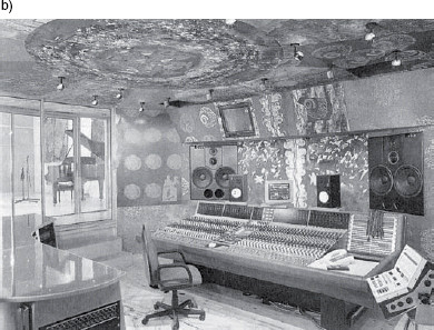
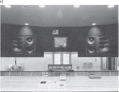
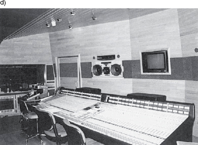
Figure 8.6 a) Garate Studios, Andoain, in the Basque region of Spain, with a Reflexion Arts 234 monitor system. b) Strongroom studios, London, UK, with a Quested Q215 loudspeaker system. c) Genelec 1035A monitor system in JVC Aydama Studios, Japan. d) Olympic Studios, London, UK, with 4-way Westlake Audio HR1 monitors
8.2.4 Crossover points
As described in Chapter 1, the maximum frequency to which a cone driver can operate with reasonable directivity control is when the wavelength is equal to the diameter of the cone. When four drivers are used in a square pattern, the group behaves at low frequencies as one large driver. When two drivers are used side-by-side, the horizontal directivity becomes that of a driver with the same width as the pair; that is, it would be narrower at higher frequencies than that of a single driver. With a vertical arrangement, the horizontal directivity may remain as it would be for one driver, whilst the vertical directivity would narrow. Depending upon the nature of the room acoustics, and whether the surfaces are absorbent or diffusive, designers must decide upon the physical distribution of the drivers, how many crossover points to use, and at which frequencies to make the transitions. The off-axis radiation will need to be as flat as possible if any significant reflected energy is likely to be returned to the listener. Wideband diffusers will return the frequency balance which impinges upon them, so a tonally coloured, non-flat off-axis response reflecting back to the listening position will tend to colour the overall perception in the room.
The general tendency is for manufacturers who sell large monitor systems for incorporation into a wide range of room designs to make multi-way systems. By splitting the frequency range into three or four bands, directivity control can be well maintained and off-axis energy can be kept relatively smooth in frequency balance. Designers who know that their loudspeakers are going to be installed in relatively absorbent rooms can concentrate on the axial response and a region of around 60 degrees in the horizontal and 30 degrees in the vertical, taking the advantage of using two-way systems which minimise the problems normally associated with crossover alignment and acoustic reconstruction. Essentially, in absorbent rooms, the off-axis energy which may be directed outside of the designated working area, and which may not have a flat frequency response due to directivity problems, is of little concern because nobody will be there to hear it and it will be absorbed at the boundaries. It therefore cannot return to the room or colour the axial response.
These concepts tend to be very poorly understood by the majority of people now working in the recording industry, and who, in ignorance, may make entirely inappropriate changes to, or of, studio systems. In so many cases, people choose their supposedly favourite loudspeakers and try to use them without any understanding of what they are really doing. It is imperative to understand that a loudspeaker system drives vibrations across a room, and that it is the combined response that is perceived. Nobody would buy a Formula One racing engine and expect it to work optimally when mounted in a tractor chassis, yet this is a close analogy of what many people do with their loudspeakers. If an axial response perception is desired, the room must be relatively absorbent. If a more lively sound is required, then the loudspeaker must be engineered to give good off-axis performance. This, as stated earlier, can have a great bearing on the choice of the number of crossover points. Fewer points tend, in general, to lead to better axial responses, whilst more crossover points tend, in general, to facilitate the engineering of a wider, more even off-axis response. However, nothing is absolute here, so designers work to find the most practical compromises for different circumstances of use.
Once that the number of ways has been decided upon, the crossover points need to be chosen. The decisions about where to cross over can be determined either by the usable frequency range of the chosen drivers, or the need to maintain a smooth off-axis response. Clearly though, where two-way systems are concerned, the chosen drivers must deal with greater frequency ranges than the drivers in systems with more crossover points. In the case of the monitor system shown in Figure 8.6(a), the crossover is placed at 1 kHz. It is unusual to operate 15 inch drivers up to such a high frequency, but the d'Appolito layout (in this case both vertically and horizontally symmetrical) and fourth order Linkwitz-Riley filters help to form a line source around the crossover frequency which is well-behaved both on-axis and over the working area. However, the low frequency drivers used in these systems are more expensive to produce than most low frequency drivers of similar size. They need to work smoothly from 1 kHz all the way down to 20 Hz – five and a half octaves. Due to the gradual decoupling of the outer regions of the cones as the frequency rises, the radiating area is progressively reduced, allowing response flatness and directivity to be maintained up to the crossover frequency. Nevertheless, the directivity change will inevitably lead to a non-flat response off-axis, so such loudspeaker designs tend to be used in rooms with absorbent side-walls.
Low frequency alignment and box size will dictate the sensitivity of the low frequency drivers. Some alignments cannot be achieved with high sensitivity drivers, but a reduction in driver sensitivity would require more power from the amplifier in order to achieve the same SPL. This fact has repercussions on amplifier choice, total power consumption, and thermal compression considerations, but, at least with large, in-built monitors, box size – and hence alignment – is not of such a critical nature as when designing smaller monitor systems.
The choice of mid-range radiators for high level monitor systems is largely dictated by function. In the low frequency part of a two-way system it is almost impossible to go from 20 Hz to beyond 1 kHz. Even to achieve 1 kHz is only possible with difficulty in physically large systems. This means that the upper frequency range from 1 kHz, or less, up to 20 kHz, or more, must be handled by one driver. If levels of 100 dB-plus are to be heard at a mixing console, 3 metres from the source, then levels of 110 dB-plus must be produced at one metre from the loudspeaker, with peaks perhaps up to 120 dB SPL. Only compression driver/horn combinations can be expected to work reliably over this frequency range as single drivers at such high sound pressure levels. The radiation pattern from horns is unlike that from pistonic radiators. Horns radiate a pattern much more like a section of a spherical expanding wave. For this reason, they can cover many octaves without the lobing which occurs when a piston begins to radiate at wavelengths which are less than its diameter. For a piston to work at 1 kHz and at levels of 110 dB SPL, it would need to be at least about 4 inches (100 mm) in diameter, if only for reasons of having a voice coil large enough to dissipate the waste heat. Given that at 20 kHz, the wavelength is only about 17 mm, a 100 mm diaphragm would be much too large for controlled radiation over a wide angle. Conversely, a 20 mm diaphragm would have no possibility of being able to dissipate 200 watts of heat from its small coil, so the requirements for radiation at such high SPLs at 1 kHz and 20 kHz are not compatible in a direct radiator.
Horns, on the other hand, exhibit much higher sensitivity. With a sensitivity of 108 dB for 1 watt at one metre, a horn loudspeaker could radiate 120 dB SPL with a total power input of only 16 watts. Given that perhaps 25 per cent of that power would actually be radiated as acoustic power, the dissipation of 12 watts of heat from a 2 inch (50 mm) coil is quite reasonable, especially given the large amount of metal in the magnet system surrounding it. Once the output from this diaphragm is squeezed through a one inch (25 mm) throat and matched to a horn of suitable size, the frequency range of 1 kHz to 20 kHz can be achieved with comfort, even at such high SPLs. A monitor system designer is therefore not totally free to choose whatever type of driver for a given system. Physical and engineering restraints limit the freedom of choice in many cases.
Although much is said about the unpopularity of horn loaded monitors in Europe, despite their wide use in the Americas, as previously mentioned in Chapter 4 many people seem to forget that the very widely used Tannoy 15 inch Dual Concentric monitors were exactly compression driver/horn loudspeakers from 1 kHz upwards. A cross-section of such a driver is shown in Figure 8.7. The monitor system shown in Figure 8.6(a) uses a horn which is relatively similar in geometry, but uses a fixed axisymmetric horn and a much more advanced compression driver with a vapour deposited beryllium diaphragm, the TAD TD 2001. Much of the criticism levelled against horn monitors was due to the misapplication of the technology and the legacy that was left from the ‘mini PA system’ monitors of the 1970s. Unfortunately it must also be added that both ignorance of what is possible, and unscrupulous comments from people marketing non-horn systems, have led many people to incorrectly believe that horn loaded upper sections in monitors cannot achieve the highest fidelity, but this is simply not true. The colouration and distortion levels of the monitor system shown in Figure 8.6(a) are extremely low, and their directivity in the type of room in which they are intended to be used is not an issue.
The system shown in Figure 8.6(b) is a three-way system, using a 3 inch (75 mm) soft-dome mid-range driver and a 1¼ inch (34 mm) dome tweeter. The crossover frequencies are set at 450 Hz and 4.5 kHz. The lower crossover point is necessary with this cone driver arrangement because the horizontally wide distribution of the total radiating area of the bass drivers would be too large to radiate wavelengths of much less than one metre, equivalent to 340 Hz, without severe directivity problems. The interference patterns would be exhibiting an excessive number of lobes, so an even directivity could not be maintained. As direct radiators can rarely be expected to span more than a decade of frequencies (or 3 octaves) the midrange driver would begin to suffer from the same problems above 5 kHz, so the 1¼ inch tweeter takes over the response for the top two octaves.
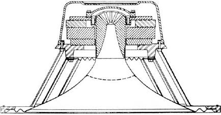
Figure 8.7 A Tannoy Dual concentric with single ferrite magnet serving for both the high and low frequency coils (see also Figure 5.10)
Figure 8.6(c) shows another three-way design, but this model can be mounted with the bass drivers either side-by-side or vertically. The sculpted panel containing the mid and high frequency drivers can be re-oriented through 90 degrees. The panel takes the form of three shallow horns, or waveguides, which serve to control the directivity of the radiation at mid and high frequencies and reduce the effect of cabinet diffraction. The midrange drivers are a pair of vertically mounted 5 inch (125 mm) cones, whilst the high frequency driver is a 1 inch (25 mm) compression driver. In this system, the crossover frequencies are 400 Hz and 3.5 kHz.
A four-way system with side-by-side bass drivers is shown in Figure 8.6(d). In this design the bass drivers only operate up to 250 Hz, from where a 10 inch (250 mm) cone driver takes over until 1000 Hz. From here on, a 2 inch (50 mm) throat, 4 inch (100 mm) diaphragm, compression driver, connected to the large wooden horn, takes the response to 4 kHz, from where a small wooden horn, fitted with a 1 inch (25 mm) throat compression driver with a 2 inch (50 mm) diaphragm continues the response to beyond 20 kHz.
From time to time, 5-way systems are also to be found, and all of these concepts from 2-way to 5-way have their applications. It should also be added that they are the results of different design philosophies which may not only reflect their intended application, but which may also reflect the order of priorities which the different designers gave to various aspects of their overall responses.
8.2.5 Power consideration
All the loudspeakers shown in Figure 8.6 are very fine systems, capable of flat responses from 30 Hz to over 20 kHz within ±2.5 dB when flush-mounted, although in many installations a high-frequency roll-off is employed for the reasons described earlier. In each case the designers have opted for different approaches to achieve what is essentially the same goal – a clean, undistorted, full-range sound, with a dynamic capability of supplying sound pressure levels at 3 or 4 metres distance far beyond what the ear can itself perceive in an undistorted manner. This excess of dynamic capability serves to allow transient headroom, damage tolerance, and reliability in long-term daily use.
However, there are big differences in system efficiency. The amplifiers normally supplied with the system in Figure 8.6(a) are specially made two-channel amplifiers, supplying 300 watts Class AG to the bass drivers and 50 watts, Dynamic Class A, to the horn. The extreme sensitivity of the horn means that at levels of 80 dB at 3 metres it would be receiving an input level of only around 10 milliwatts, so the low-level performance of the amplifier is extremely important. The Class A design was chosen to ensure the absence of low-level crossover distortion. Even at 100 dB at 3 metres, only about 1 watt is consumed by the mid/high driver, with the low frequency driver taking around 20 watts. This is a very high efficiency system, in which thermal compression is almost non-existent due to the low power levels and the high thermal capacity of the large magnet systems. A stereo pair, without signal, draws about 0.4 amps from a 230 volt supply (92 watts) and at full power 4 amps (920 watts).
Some designers feel that by using drivers of lower sensitivity they can better achieve their design goals. The systems shown in Figures 8.6(b) and 8.6(c) use amplifiers with output capabilities of over 2.5 kilowatts per side, a stereo pair requiring at least a 30 amp supply from 230 volts mains. The four-way system shown in Figure 8.6(d) uses medium and high sensitivity drive units, and a pair can operate comfortably from a 10 amp supply.
In all cases, though, oversized power cables should be used in order to keep the supply impedance down. Some amplifiers can draw current in surges, which can instantaneously drop the voltage of supplies without an adequately low impedance. Not only can this rob the bass of transient punch, but the harmonics created by the change in waveform as the voltage sags can cause problems in associated equipment, and can even crash computers. It is best to supply the amplifiers with their own, dedicated supply cable or cables, fed straight from the incoming mains supply at the main circuit breaker board. The breakers feeding the amplifiers may need to be of the delayed action type, because some amplifiers draw high surge currents on switch-on.
The question of total power consumption can be important. In hot countries, such as in southern Europe, it can be difficult to dissipate heat when it is 40°C in the shade. In many places, high current supplies to buildings are hard to organise, and when an extra 2 kVA of air conditioning is needed, just to cool the amplifiers, it can put a great strain on the whole studio electrical installation. Many people have said that it can be cheaper to make low efficiency systems because magnets are expensive and amplifier power is cheap. Well, it is cheap to buy the amplifiers, but the running costs over years can be very expensive indeed when system efficiency is low. Depending upon circumstances, things such as this may or may not be important to the users, but they nonetheless need to be considered because the electricity bills and the heat production cannot be ignored.
There is also a tendency for higher sensitivity systems to exhibit faster transient responses due to the more stable static magnetic fields which are a part of their general character. Computer-aided loudspeaker design programs can often call for lower sensitivity drivers in order to achieve certain design aims, but ears can sometimes ask for something different. One has to be very careful when balancing design parameters if one is not to gain in one department but lose in another. This all tends to be a question of there being too many design parameters which may affect audible responses but which are not available for incorporation into the computer-aided design processes. So, if the whole story does not go in, then it is unlikely that the whole story will come out.
The monitors shown in Figure 8.2(a) are interesting in that they are twoway but use high level passive crossovers. The pair of 16 inch (400 mm) bass drivers operate up to about 300 Hz, with the compression driver handling the upper six octaves. The dynamic impedance can dip to as low as 0.8 ohms at some frequencies and under some drive conditions, and can demand as much as 100 amps (peak) from the amplifiers. Very few amplifiers can deliver this amount of output current, and those that can tend to be very expensive indeed. These monitors are frequently used with FM Acoustics, or JDF amplifiers, which can deliver 3000 watts into half an ohm. In 2000, the price was around 100,000 dollars per pair for the loudspeakers, amplifiers and cables, the latter of which cost around 2500 dollars per side. The demands on the cables are obviously great, and bi-wiring is standards. With the cable to the horn carrying six octaves and the low frequency cable up to 100 amps, the prospects for intermodulation in a single cable would be considerable. The crossover components are also large and expensive, with oxygen-free copper inductor coils.
The engineering of such systems is not a simple task. In fact, despite initially appearing to be the simpler solution, the high-level passive crossover option can be extremely difficult to implement if the highest achievable sound quality is the goal. Multi-amplification actually simplifies many things, even though it perhaps initially seems to be a more complicated approach. However, in the above case, the designer Shozo Kinoshita, in his experienced view, chose the passive crossover option.
One of the largest commercial monitor systems is shown in Figure 8.8. The Quested HM 415 loudspeaker weighs about a quarter of a ton, and the maximum output is claimed to be 130 dB SPL at one metre. The bass units are four 15 inch drivers with external chassis, which help to improve the cooling of the voice coils. The low mid-range driver is a 7 inch (175 mm), rigid, polyurethane foam dome. The high mids are radiated via a 2 inch (50 mm) soft dome, and the high frequencies radiate from a 28 mm dome. The amplifier system uses 5 channels, the bass being split into two parallel channels, and the full power consumption is 3.5 kVA per channel from the electrical supply for 2400 watts of output power.
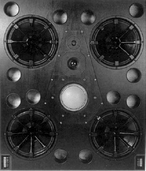
Figure 8.8 The enormous Quested HM415, 1 m 26 in height, 1 m 06 in width, and weighing over 260 kg, using a combination of rigid-dome and soft-dome radiators in the mid-range. Each 15 inch (380 mm) low frequency driver is in its own triple-ported chamber. The external chassis of the LF drivers aid the cooling of the voice coils. The systems are rated to deliver 130 dB SPL at one metre distance
8.2.6 Interfacing with the rooms
The ‘high-end’ recording monitor systems such as the ones described above are the ‘Formula One’ of monitoring. However, just as the thoroughbred racing cars need a good track to race on, the high-end monitor systems need to be mounted in well designed rooms. Formula One racing cars cannot perform on rough roads, and neither can the top monitor systems perform in poor rooms. As we get further into the discussion of loudspeakers for different applications we will begin to deal with loudspeaker designs which are intended to be more room-tolerant, but the larger systems, partly due to their physical size and widely spaced distributions of the drivers, cannot be considered to be particularly room tolerant. It is therefore entirely unreasonable to make judgements about the sound quality of such systems in rooms which cannot do them justice. It is sad to say that many comments which are heard in the recording industry, relating to large monitors, are based on pure ignorance, or bad experiences of misapplication.
Unfortunately, the requirement for the necessary degree of room control in order to be able to mix on the large monitors means that the total cost of providing such a facility is not something that everybody can afford. Large monitor systems in small rooms can be overpowering, because it can be impossible to get them far enough away from the listening position to avoid geometrical near-field effects, where the sound is heard from individual drivers, and not an integrated source. Figure 8.9 shows a scaled down system in a small control room, albeit still in large, 200L cabinets (6 cubic feet). To use any of the systems shown in Figure 8.6 in such a small room would be absurd. The use of such large systems only begins to become viable in rooms of 40 to 50 m2, which would perhaps leave 30 to 35 m2 of useable space after treatment. When the cost of the monitor system and acoustic control for such a room would perhaps begin at around 40,000 euros, many studio owners decide that it is difficult to get a return on the investment. Nevertheless, the larger studios understand the importance of the recording monitors where engineering excellence is concerned. Marketing only really seeks to achieve the maximum profit for a given investment, whereas professionals and artistes seek to earn a living from doing what they do to the best of their ability, and the maximisation of the financial returns are not their sole concern. The pressures to find less expensive solutions are nowadays very great, but it still needs to be understood that just because something cannot be afforded does not mean that it is not necessary!
The tendency to use near-field, or, more properly close-field monitors is often simply an attempt to take the room out of the monitoring equation. One problem with this approach is that there is not much room for more than one or two people to hear the optimum sound, and what is more, the frequency range of the small loudspeakers is necessarily curtailed at the lower end of the frequency spectrum. (Sub-woofers rarely yield accurate bass, as will be discussed in later chapters.) The close-field is the space within the critical distance – the critical distance being that at which the energy which is contributed to the overall sound is equally supplied by the direct and reflected sound fields. It thus follows that as the room decay time is reduced, the close-field increases in size. The high degrees of absorption in some control room designs thus seeks to extend the close-field of the large monitors all the way to the listening position. This effectively yields a close-field response but with a greater optimum listening area. [The acoustic near fields, strictly speaking, both geometric and hydrodynamic, are regions very close to the loudspeakers where a highly complex, unintegrated sound-field exists, and where the composite sound that we hear in the far-field has not had time or space to jel into an integrated wavefront. Listening to the monitors shown in Figure 8.6(d) at a distance of one metre would be a typical example – the physical distribution of the individual sources would audibly be very evident.]
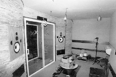
Figure 8.9 A small control room, under construction in Ubeda, Spain, with a miniaturised Reflexion Arts 240c system. The cabinets are large, to allow a generous and fast low frequency response, but the drivers form a compact group to minimise the geometrical near-field problems at short listening distances. The rear wall, side walls and ceiling are highly absorbent behind their fabric coverings
There is also a lot of nonsense spoken about control rooms, especially by people who are just repeating hearsay; and it has to be said that the marketing pressures lead to some very partisan passing of opinions which are little more than attempts to gain a commercial advantage. Clearly, the majority of studio owners who cannot afford good control room acoustics and large monitors are rarely going to admit that their studios would be much better if they could afford them, so the received wisdom about these things often has little to do with fact. Comments that well-controlled rooms are not necessary should be treated with suspicion. If such things were not necessary, then why would almost all the top studios have them?
8.2.7 A word about listening levels
Some people may be shocked reading about listening levels of 100 dB, or more, when so much safety information now restricts industrial levels to 95 dBA or less. However, as the levels within symphony orchestras can easily exceed 95 dBA or 100 dBC (the C-weighting measuring more of the bass) it would seem to suggest that all orchestral musicians should be deaf after a few years of work. This is patently not in accordance with the reality, as most experienced classical musicians exhibit excellent hearing acuity. It also follows that if the performance levels do not damage the ears, (except in some cases where musicians play directly in front of the trumpets), then the loudspeaker reproduction of such ‘natural’ levels should also lead to similar results.
Hammer blows, on the other hand, despite only reading 95 dBA on a sound level meter can produce rapid peaks of 135 dBA or more, but they are too short for the meters to read. It is these peaks which damage the hair cells in the ears, but the more rounded waveforms of music rarely contain any peaks so far above the measured levels. Therefore, whilst mixing is not recommended to be carried out at such high levels, for many perceptual reasons, it is still not unreasonable to work during the recordings at the realistic acoustic levels experienced by the musicians. Drum kits would have already been banned in many countries, for health and safety reasons, if a short career as a drummer automatically led to deafness. Classical soprano singers can also produce over 120 dBA one metre from their mouths, and this is why many good recording engineers never place a recording microphone closer than one metre from a soprano – to save the microphones from overload – yet there are few reports of people being deafened by sopranos. Nevertheless, it is still wise to only monitor loudly when deemed necessary, and not to make a habit of doing so if not required. Perceptually, also, mixing is better carried out at levels more close to end user reproduction levels, but that will be dealt with in the next section.
8.3 Mixing monitors
Once we arrive at the stage of mixing the multitrack recording down to stereo, or surround-sound, we are no longer in an environment where we can affect the performance of a piece of music. Stimulating the musical performance is no longer either necessary or possible, although ‘vibing’ the mixing personnel, who are still very much a part of the creative process, is still a possibility. A quick blast at 105 dB can, at times, be very satisfying, but mixing at such levels is rarely a good idea. The equal loudness contours shown in Figure 8.4 demonstrate clearly how at different listening levels we perceive different frequency balances. In general, when people are listening to music at home, they tend to listen between 75 and 85 dB SPL. The dBC weighting curve which is used on many sound level meters represents something very similar to the inverse of the 80 phon curve of Figure 8.4. (The more common dBA curve being similar to the inverse of the 40 phon curve – used for the assessment of background noise nuisance.) In Figure 8.10, the 100 phon curve has been superimposed on the 70 phon curve. If we mix at 100 dB SPL, then listen at 70 dB SPL, the perception of the low and high frequencies relative to the mid-frequencies will change by the difference between the curves. A mix which seems balanced in frequency at 100 dB SPL will sound at 70 dB SPL like the bass should have been mixed 3 or 4 decibels higher, and it may sound somewhat dull due to the ear's lower sensitivity to the treble frequencies. Mixing at high levels is therefore unlikely to lead to well-balanced mixes at normal listening levels. Furthermore, mixing at 100 dB SPL plus for day after day will almost surely lead to serious hearing fatigue. It will also lead to temporary shifts in the hearing threshold as the ear's protection mechanisms come into play, and normal perception will not be possible. In fact, from the hearing sensitivity contours shown in Figure 8.4, it can be seen that the contours tend close up at low levels of low frequencies. Despite the fact that 10 dB is generally considered to double loudness, it can be seen that at 70 dB SPL and at 40 Hz there is only about 4 dB between the adjacent loudness doubling/halving contour lines. This implies that a 4 dB difference in overall level at 70 dB SPL may subjectively double or halve the relative loudness of low frequencies, whilst the mid frequency loudness would change by a much lesser amount. This is another reason to avoid mixing at much higher levels than the expected reproduction levels, because the low-frequency/mid-frequency relative balance will be difficult to judge in relation to how it will generally be perceived domestically.
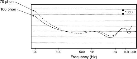
Figure 8.10 The 70 and 100 phon curves overlayed to coincide at 1 kHz. Note that they coincide elsewhere only at around 200 Hz and 6 kHz. At the frequency extremes they differ by as much as 10 dB, with the ear being more sensitive low frequencies at the higher SPL but less sensitive to the 15 kHz region. The way that the curve intertwine does not make the prospects of automatic correction a very practicable proposition
Mixing also tends to be a much more continuous process than recording, so sustained high level mixing can lead to more problems than high level monitoring during recording. Even if recording engineers do animate musicians or look for noises at 105 dB SPL, they probably would not be exposed to such levels for more than about an hour a day, and in short bursts at that. And, despite ‘common knowledge’ about recording engineers being deaf, there is no evidence to support that idea. Most of them have very acute hearing, which they probably take care of more than most other people do. [DJs, – well, that is another matter!]
In the world of mixing cinema soundtracks, the monitor volume level is fixed, to guarantee that the audiences in the cinemas hear the same level, and hence frequency balance, as the mixing personnel in the studio dubbing theatres. This is a luxury which cannot be enjoyed by music mixers, but, as few people will listen seriously in their homes at either 60 dB SPL or 100 dB SPL, an 80 to 90 dB SPL mixing level seems quite reasonable, or a little lower or higher if desired.
Mixing monitors therefore do not need to be capable of the same output levels as the recording monitors, and this fact can be significant. Ten decibels less in peak output capability means ten times less power handling capacity if the same sensitivity of drive units are used. This could make the engineering much simpler and the area occupied by the drivers more compact. However, the tendency is to use physically smaller loudspeaker cabinets at closer listening ranges. Essentially, what the mixing personnel are trying to do, subconsciously or otherwise, is to remove the room response from the listening chain. To move the loudspeaker close is a much cheaper alternative to treating the room. However, the smaller cabinets require less sensitive drive units if the bass response is to be maintained, (as was described in Chapter 3) so the amplifier power still needs to be quite considerable in many cases, even to work at a maximum average level of 100 dB SPL at 1.5 metres distance. It also means that some of the potential advantages of using much lower powers are not realised, so thermal problems arising from needing to lose the same amount of heat from smaller drive units can have its repercussions on design priorities. In some cases, sensitivities as low as 81 or 82 dB for one watt at one metre are encountered, whereas it is rare indeed to find recording monitors with sensitivities below the 90 dB sensitivity level. The widely used UREI 815s of the 1980s had sensitivities of 103 dB for one watt at one metre. Figure 8.11 shows the two extremes. Obviously, when the smaller loudspeaker needs almost 200 times the power (22 dB) that the large ones need to produce the same SPL, the engineering considerations can be very different in the two cases. Such are the problems that face loudspeaker designers.
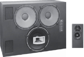
Figure 8.11 The Urei 815 and ATC SCM10 loudspeaker systems. The smaller loudspeaker needs an input of almost 200 watts to develop 103 dB SPL at one metre distance. The UREI 815 will achieve the same SPL with an input of only 1 watt
For many people, mixing is an insecure process. Some of the reasons why will be discussed in Chapter 10, but some of the insecurity is reduced by following fashions in the choice of mixing loudspeakers. In the rock music world, the Yamaha NS10M served as an unofficial reference standard for twenty years or more. Of course, to become an international standard, even if unofficially, the loudspeakers need to be internationally available, so the offerings of large companies tend to be favoured rather than the use of locally manufactured brands – even if their performances are similar. Nevertheless, it is not all down to fashion and marketing. There is usually some reason why so many people in so many places gravitate towards certain monitor loudspeakers out of the plethora available to them. Some manufacturers have made studies of hundreds of loudspeaker responses, both professional and domestic, and concluded that a loudspeaker which exhibits something close to the mean response will be likely to succeed as a mixing monitor. However, that work applies only to the frequency response amplitude, but there are many more qualities which people look for during music mixing.
Domestic loudspeakers are usually inadequate for music mixing because they lack the robustness to withstand such operations as the soloing of bass drums, which are essential during the mixing process. Characteristics such as absolute sound quality and the ability to give a realistic response under the conditions of use found in mixing rooms are aspects of mixing monitor performance which may differ very significantly from the requirements of use found in most domestic environments. It is rare, for example, for people to listen seriously to music with the loudspeakers placed on top of the far side of the dining-room table, but this would not be too unlike the placing of loudspeakers on top of a mixing console. Therefore, for professional mixing purposes, the desired anechoic response must take into account the mounting conditions under which the loudspeakers will actually be used if reasonably accurate mixes are to be created.
The aforementioned dominance of the NS10M as a mixing monitor for pop/rock/electronic music, over so many years, was surely in part due to the fact that it exhibited a tendency for its overall response to flatten when placed on top of a mixing console – its predominant position of use. Figure 8.12 shows the gradual change in an NS10’s response as a mixing console and room are brought into its proximity. From these results it should be apparent that mounting mixing loudspeakers on a meter bridge or on pedestals are not alternative options. A mixing console will augment the low frequencies but a pedestal will not. The decisions must be made according to the designers’ intentions, and the local boundary conditions presented by the rooms unless the monitors are self-powered, and fitted with tilt and roll-off controls to compensate for the acoustic loading differences. Far too many people, even professional mixers, fail to realise that the loudspeaker and its mounting conditions cannot be separated. No fixed response loudspeaker is suitable for all mounting conditions.
The NS10’s popularity was also probably due to the fast and uniform decay of its time response. Figure 8.13 shows a selection of waterfall plots from nine different mixing monitors. The similarity of the plots of the NS10M and Auratone 5C are too close to be mere coincidence. The Aura-tone was one of the first, internationally used ‘references’ – originally used as a small loudspeaker reference in the days when the large monitors were still the most commonly used mixing loudspeakers. The NS10s very largely displaced the Auratones when they arrived on the scene in the early 1980s. They exhibited a considerably wider frequency response and significantly more output capability, yet still maintained the response characteristics that made the Auratone 5C so popular. The deeper consequences of their responses will be discussed further in Chapter 11, but it can be seen from Figures 8.12 and 8.13 that their responses were tending towards flat and fast when placed on top of mixing consoles, and these two characteristics are conducive to good mixing. Basically, if one could ignore the colouration, and check the low frequencies on other systems, the NS10s and 5Cs told many mixing engineers what they needed to know in order to make a good balance of instruments and reverberation.
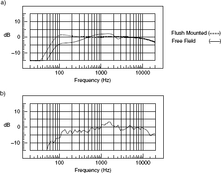
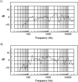
Figure 8.12 a) Response of idealised loudspeaker: flush mounted (dashed line) and free-field (solid line). b) Response of Yamaha NS10M, outside, flown 4 m from floor and wall. c) As b), but mounted on a mixing console metre bridge (all flow 4 m from ground). d) As c), but with the mixing console on the floor in a reasonably controlled room. Note how the overall response gradually changes – (b) shows a response rather similar to the free-field response in (a), whereas (d) shows a response more similar to the flush-mounted response in (a)
The twin demands of lowering production costs and maximising the commercial acceptance of the mixes have led to a situation where by far the majority of music is mixed on relatively small monitor systems, a selection of which is shown in Figure 8.14. Although fashion plays a big role in the choice of which loudspeakers to use, and some commonality of choice is still to be found, there are nonetheless many individual choices made by different people, and it is not by any means unusual to hear discussion between people who cannot understand how each other can use their loudspeakers of choice. Many of the differences come down to different hierarchies of priorities and methods of working – which both ultimately translate to individual ways of thinking about the work. Mixing-loudspeaker characteristics can be separated into parameters such as spectral uniformity, dynamic performance (transients), distortion, sound-stage imaging, off-axis performance (very relevant in less controlled rooms), ambience reproduction (transparency), and, of course, the overall impression. However, the order of these characteristics will not be the same for all people. And, what is more, work and leisure requirements may be very different. Many top recording engineers, mixers and producers do not use the same loudspeakers at home that they use in the studios, even though the sizes of the loudspeakers may be similar. At work, they need to hear all the problems; at home, they simply want to enjoy the music. But another reason for the difference is because, in general, almost all serious mixing will be done in rooms with a reasonable degree of acoustic control and a lot of equipment, whereas acoustic control usually does not take much precedence in the designs of their homes, and domestic furniture tends to be rather acoustically different to mixing consoles and equipment racks. The object of the exercise is therefore to do mixes in a professional environment which will translate to a domestic environment. The recording engineers’ homes also furnish them with a means of listening as other people listen, which helps them to get another perspective on their work. For these reasons, mixing monitors for use in studios have developed along their own course.
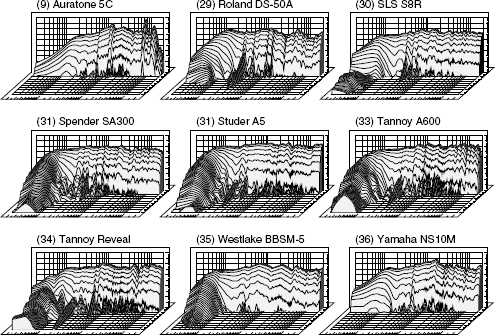
Figure 8.13 Nine waterfall plots – all of close-field monitor loudspeakers in an anechoic chamber
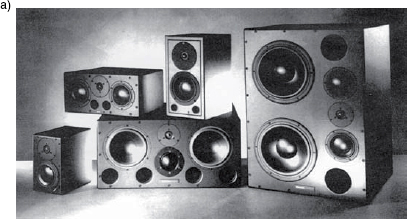
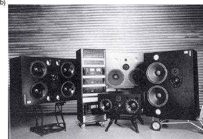
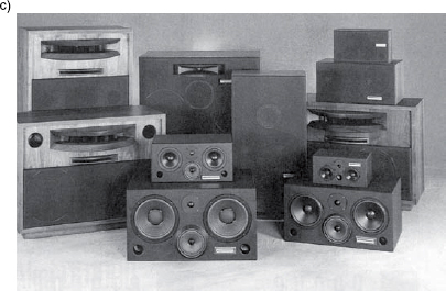
Figure 8.14 Three families of studio monitor loudspeakers. a) Dynaudio Acoustics systems b) Quested Monitoring systems. c) Westlake Audio systems
In a report presented in 2004 relating to the selection of a new ‘standard’ choice of monitors for the BBC2, the author acknowledged; “Loudspeakers are a sensitive topic on which many people have very different views.....” Despite this, however, in an organisation such as the BBC, with over 600 sound control rooms, some standardisation is necessary because the staff need to move around from room to room, but always need to know what they are listening to. They also use rooms which are rather more dead than most domestic rooms because ‘Critical assessment of sound quality cannot be carried out in rooms with large areas of specularly-reflecting surfaces and long and uneven reverberation times, however attractive they might be architecturally2’. As we will discuss later, domestic loudspeakers must deal with these conditions, but they really cannot replace professional loudspeakers if a good degree of consistency of sound quality is required when used in typical mixing environments.
The BBC carried out their tests in rooms with a mid-band decay time of about 0.2 seconds, which is quite typical of modern control rooms, but it is much lower than is normally to be found in most domestic rooms. The listening tests were carried out during a period of three weeks, by eleven ‘democratically chosen’ representatives of the staff – all very experienced listeners – on a total of 28 pairs of loudspeakers. In the ‘Summary and Conclusions’ of the abovementioned report it stated “Inevitably, the final outcome was not entirely clear-cut.” The tests were made using large, medium and small loudspeakers, without the listeners knowing the identity of any of them. It is interesting to note that no set of three from any one manufacturer stood out from the rest in either quality or family resemblance. The best family resemblance of a large, medium and small loudspeaker was of mixed manufacturer.
8.3.1 Location dilemmas
The main purpose of the mixing monitors is to reliably enable the mixing personnel to achieve musically and timbrally balanced mixes. Working in the close-field, if the loudspeakers are too small and their low frequency responses are too restricted, then the lower octaves may be leading an uncontrolled life of their own due to the inability to monitor them. Adding shelf equalisation to an instrument at 80 Hz may give rise to unintentional rises at 30 or 40 Hz, leading the mixing personnel to believe that they have obtained the desired tonal balance which subsequently, when played on larger loudspeakers, turns out not to be the case. The use of larger loudspeakers for the mixing may mean pedestal mounting, behind the mixing console, but unless the back of the console is heavily treated with absorbent material, the reflexions from the rear surface can ricochet around the room, affecting the clarity and stereo imaging. This concept of ‘mid-field’ monitoring also brings more of the room acoustics into the listening equation, and the omnidirectional low frequencies will rarely be as flat as from monitors flush mounted in the wall, which do not suffer from the reflexions of rear radiation and the subsequently response irregularity due to interference at the listening position. Neither will the low frequencies from mid-field monitors be as likely to be as flat as the ones that are available (to a more restricted degree, of course) from loudspeakers mounted in the close-field, where the direct sound dominates the overall response. The whole situation is full of frequently irreconcilable compromises, and great experience may be required in deciding just how the most workable compromises can be achieved.
There is, of course, no fixed response for all mixes. The mixes are, above all, artistic interpretations of the performances which they encapsulate, so if a certain type of loudspeaker leads a certain mixer or producer to achieve their desired results, then those loudspeakers will, for them, be excellent mixing monitors, even though for other people they might be considered to be unusable. Nonetheless, in general, achieving a smooth response at the listening position is still a highly desirable goal.
Mixing monitors are therefore a means to an end, and not an end in themselves. They are tools, and just as with any other tool, such as a tennis racquet or a pair of football boots, different models may suit different individual styles of use and personal comfort. However, it is indeed rare to find normal domestic hi-fi loudspeakers in use as mixing monitors, or typical mixing monitors in use as domestic hi-fi loudspeakers, because they are used quite differently and in acoustically different circumstances. But in a growing number of cases, yet another type of loudspeaker has been introduced into the chain to try to interface better the professional and domestic worlds, which we shall now look at in a little more detail.
8.4 Mastering loudspeakers
Historically, the last stage of the quality control of the recording process, both artistic and technical, was the disc cutting, when the tapes were transcribed to cellulose acetate discs. From these discs the stampers would be made, by processes of electroplating, which would in turn mould the vinyl records for sale in the shops. Once all the settings had been decided upon, and a written record had been made for future reference, an acetate test cut could be taken home, or to the record company offices, to assess the sound in known, domestic-type conditions, which were considered to be more representative of end-user conditions than the machinery filled space of the disc cutting room. If all sounded well, the engineers or producers could return to the cutting room, adjust the equipment once more to the settings which had been written down, and a master disc could be cut and sent to the factory. (It was important not to play this disc, as the soft acetate was easily damaged.) If it was felt that some adjustment needed to be made to the sound, then the appropriate changes could be made to the settings of the equalisers or compressors before the final disc was cut.
Reference acetates were also frequently cut to assess tracking, because what could be cut on to disc was not always able to be played back on cheaper domestic equipment. The cheaper cartridges could not always keep their styli in the grooves if they were too heavily modulated, and customers would return the discs to the shops if ‘the needle jumped’, which could be very expensive for the record companies in lost sales. Vinyl discs therefore always had to be made to a realistic lowest common denominator, and it was not only the stylus tracking which made this necessary. In the 1970s and early ’80s most domestic loudspeakers were not capable of supplying high levels of low frequencies, so excessive bass levels could either cause distortion on playback or cause the listeners to turn down the bass on the tone controls of their equipment. In neither case would they be hearing what the people recording the disc were intending them to hear, so the artistic intention of the disc could not be fulfilled. Once again, it would be an acetate test disc that would usually be used to confirm the overall domestic compatibility of the musical mix.
With the advent of the compact disc, the greater capabilities of digital recording introduced low frequency response possibilities that were never available from vinyl discs or tape cassettes, and the domestic loudspeaker manufacturers began to respond with more robust loudspeaker systems which could highlight the new advantages of digital recording. Music mixes then needed to be prepared for multi-format release, on vinyl disc, compact disc and tape cassette, and producers still wanted to know, as ever, what the mixes would sound like on the radio. The early 1980s therefore began to see the birth of a new concept within the recording chain; the concept of the mastering studios, where all of these questions could be resolved.
Mastering engineers tend to always work in the same place – their own dedicated mastering room. Their rooms, equipped with their own choices of loudspeakers and equipment become their references. During the course of a year, many more recordings will usually pass through a mastering room than a mixing room, and the recordings which a mastering engineer deals with are likely to vary, in terms of musical styles and recorded quality, much more than the recordings worked on by a mixing engineer. Consequently, mastering engineers gain much experience about how a very wide range of recordings sound in their own, personal rooms. In general, mastering rooms are much more sparsely equipped than mixing rooms. There is usually no mixing console between the loudspeakers and the listeners, and what furniture there may be tends to be of an open and not very reflective nature.
Mastering is the last chance to solve problems, or at least to be aware of them before the music goes to the factories and the shops. It is therefore necessary at this stage to be able to listen critically, both artistically and technically. With experience, mastering engineers get to know the relationship between how things sound in their own rooms and how things sound in a wide range of circumstances in the outside world.
Mastering rooms often have acoustic properties somewhere between the typical studio control room acoustics and typical (if such a thing exists) domestic replay circumstances. The monitor systems which they use are frequently of wider frequency range than many mixing monitors, because the mastering personnel need to be able to look for things that have been neglected in the mixing circumstances, and they often do this by using larger loudspeakers which are either not of the reflex design, or are reflex boxes with very low tuning frequencies. Mastering monitors can often afford to be larger because they do not need to fit into the spaces left after the mixing console and equipment racks have been installed – both of which are very necessary for mixing purposes. A typical mastering room is shown in Figure 8.15.
The great tendency is to use free-standing loudspeakers, because many mastering engineers feel that these are more typical of the way in which the music will be perceived in the domestic circumstances. The larger boxes and lower low frequency responses facilitate the assessment of the low frequency colouration, and reduce the masking effect which can cover low-level detail when reflex cabinets of a higher tuning frequency are used. Furthermore, the mastering studios need to be able to cope with whatever work comes to them, and if some work is of a very high quality, extended low frequency nature, they need to be able to hear it at its best, because guessing is not what mastering engineers are paid for. Their job, to a very great degree, is to give confidence to the rest of the people who have been working on the performances, recording, mixing and editing of the music, and also to the record companies who may be distributing it. For the above reasons, mastering loudspeakers tend to be of an audiophile high fidelity quality, which are capable of being used in rooms with an acoustic which is often less controlled than the studios in which the mixes have been made. Mastering monitors are not required to support the stresses of solo'd drums or bass guitars, so they generally do not need to be as robust as recording or mixing monitors. This fact can allow mastering engineer's greater flexibility in their choice of loudspeakers.
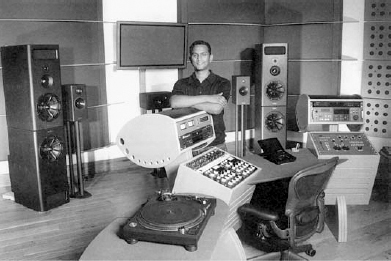
Figure 8.15 A typical mastering room arrangement. Optimum Mastering, Bristol, UK, with engineer Shawn Joseph and a pair of large PMC transmission lines
From time to time, however, one encounters mastering studios which are more like a recording studio control room, but with some notable modifications. The room shown in Figure 8.16 is based on a control room design, but with the loudspeakers mounted in such a way to maximise the accurate listening area, as no compromises need to be made to accommodate a mixing console. The flush-mounted loudspeakers, although of a type used in smaller control rooms, will normally not be used at control room levels, because mastering engineers tend to work at domestic levels, so the high frequency roll-off that would be applied if they were in a recording studio (as discussed in Section 8.2) is left flat. The owner of the mastering room shown in Figure 8.16 is a former recording engineer who feels the need to be able to refer to a more typical, recording-style, full-range monitor when needed, and uses a smaller set of monitors as a secondary reference. As in all matters associated with loudspeaker choice, no absolute, hard and fast rules apply, though strong trends are apparent.
Figure 8.17 shows yet another mastering room. In this case the monitors consist of loudspeakers on stands but with a dedicated sub-woofer below each one. These sub-woofers come into use below about 80 Hz, where the directional characteristics of the auditory system are very poor. This allows the mastering engineer to use full-range monitors, but of smaller physical size than those shown in Figure 8.15. The room is used for much work in surround sound, and the owner felt that five large, full-range loudspeaker boxes would cause too many acoustic problems if they were surrounding him at close range; especially when only working in 2-channel stereo. However, it is important to note that the sub-woofers are not used with any arbitrary bass management system. They are only used for extending the low frequency responses of the loudspeakers which are mounted above them. There are therefore five sub-woofers for five loudspeaker channels.
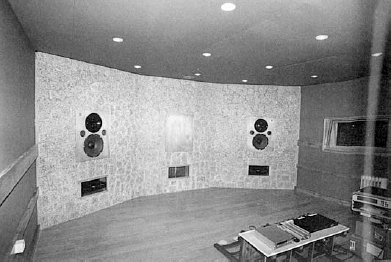
Figure 8.16 A mastering room prepared for a future, centre-front loudspeaker
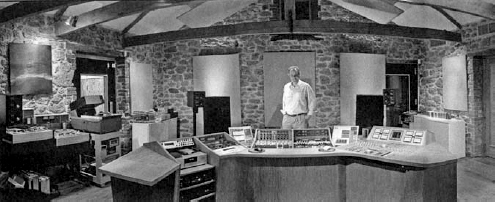
Figure 8.17 Super Audio Mastering – Chagford, Devon, UK
There is a significant difference between the responses of small cabinets with sub-woofers below, and larger full-range, integrated cabinets when free-standing in rooms. Although the on-axis responses may be the same in either case, the greater mid/high frequency diffraction of the smaller cabinets gives rise to more reverberant energy in those frequency bands than would arise from generally larger cabinets. In semi-reverberant conditions, typical of many mastering rooms, this gives rise to a better balanced reverberant response compared to the somewhat bass-heavy reverberation which is typical from the larger cabinets, whose greater front baffle areas restrict the mid/high-frequency diffraction. Obviously, though, in a more absorbent general acoustic, the difference would be less noticeable at the listening position, so once again the choice of loudspeaker designs is very closely linked to the rooms in which they will be used.
It is often said by mastering engineers that the loudspeakers which are used for the great majority of music mixing are not sufficiently revealing of low-level details, whereas mixing engineers say that the loudspeakers typically used for mastering are difficult to use for mixing because they do not interface well with the equipment distribution of a mixing studio. They also often speak about the difficulty of mixing on loudspeakers which reveal too much detail, because the information overload becomes an obstacle to concentrating on the mix, and that smaller loudspeakers give a more close approximation to typical end-use conditions. It is interesting to remember that in the 1960s and early 1970s, the people who mixed the music were often referred to as balance engineers, and that musical balance is the essence of good mixing.
What is very clear therefore is that whilst recording, mixing and mastering can all be accomplished on one set of loudspeakers in one room, there are operational and financial reasons why the use of different loud speakers and acoustic conditions can be beneficial at each stage of the process, and that recordings which have passed through those different stages are perhaps better prepared for the very wide range of circumstances in which they will ultimately be heard in peoples’ homes.
8.5 Domestic loudspeakers
The scope of domestic loudspeaker design and performance is enormous. Some of the audiophile designs cost more than even the largest recording monitors, whilst the smallest and cheapest are perhaps those in a typical ‘ghetto blaster’ or portable music centre. All, however, ostensibly serve one purpose – to give enjoyment to the listeners when reproducing music, either recorded or via live broadcast. The range is vast because the degree of importance which people give to listening to music is also very great, from fanatical to inconsequential, and also because the homes in which music will be heard can be architecturally very different. It was recognised a long time ago that many Californian designers of hi-fi loudspeakers aimed for different low frequency alignments than many British designers, because the typical wooden framed houses of California responded very differently to the musical signals than did the solid, stone or brick houses in the UK.
Rooms which are heavily endowed with soft furnishing will be absorbent in the higher frequency ranges. As most domestic listening takes place in the far-field, where the reflected response dominates the direct response from the loudspeakers, a loudspeaker with a brighter anechoic response may sound better balanced in some homes than a loudspeaker with a flatter axial response. Loudspeakers placed against walls or near to corners will exhibit a much reinforced bass response compared to loudspeakers which are placed away from reflective boundaries. A flat loudspeaker may therefore sound bass heavy when close to a reflective boundary, so a choice of loudspeaker with a reduced low frequency response may sound more balanced in such circumstances. In many cases, for reasons of domestic harmony, loudspeakers may have to be placed in conditions which would not suit those having flat anechoic responses, so the range of different loudspeakers available to the public can offer a choice to select a model which best matches the circumstances of use and the affordable price range. It is therefore essential to judge domestic loudspeakers at home for final assessment, unless the acoustic conditions and mounting conditions in the showroom are very close to the conditions of use. And, of course, one should never be reluctant to use any tone controls on the amplifiers to make a final adjustment to taste. The concept that the tone controls should be left flat for a maximally accurate sound to be heard is absurd, unless the listener lives in identical conditions to those in which the recordings were mixed or mastered.
Low colouration, low non-linear distortion, a smooth frequency response which tends towards flat in conditions of use, and an adequate dynamic range are all common goals for either recording, mixing, mastering or domestic hi-fi loudspeakers. However, the fact that in the latter case the acoustic conditions of the rooms in which they will be used will almost never be based on the requirements for the loudspeakers; the loudspeakers must be chosen to suit the rooms, whereas in the former, professional cases the rooms are often treated to accommodate the loudspeakers. For this reason, whereas professional loudspeakers tend towards similarity, the domestic loudspeakers tend towards diversity. The first book mentioned in the Bibliography at the end of this chapter deals with the subject in more depth, and those 500+ pages only deal with high performance loudspeakers, which gives an indication of the scope of domestic loudspeaker design.
Taste is also an allowable parameter in the selection of domestic loudspeakers to a much greater degree than in professional loudspeaker choice. As was mentioned earlier in the chapter, most professionals in the music recording industry do not use at home the loudspeakers that they use at work. Very few people, except some audiophile die-hards, want to hear every error and distortion in a recording when they are listening for pleasure. There is therefore an incentive for the manufacturers of domestic loudspeakers to make products which sound pleasant, even at the expense of accuracy. This is a totally reasonable situation in the design of products which are, after all, intended to be used for enjoyment. Nevertheless, the same basic principles apply to the majority of the four categories of loudspeakers discussed so far. On the other hand, for the final group of loudspeakers to be discussed in this chapter, sounding pleasant is their only function, and in their design just about everything that we have discussed so far is about to be turned on its head.
8.6 Musical instrument loudspeakers
As mentioned at the beginning of the chapter, loudspeakers for musical instrument amplification are part of a music production process, not a reproduction process. Reproduction by loudspeakers can be classified as a situation where the acoustical output is intended to accurately represent the electrical input. Conversely, in music production loudspeakers, the controlling factor is the subjectively desirable nature of the output sound, irrespective of its relationship to the electrical input signal.
A bass guitar, for example, has a very dynamic output. The peak-to-mean ratio of the signal is very great, and if a bass guitar is directly injected into a mixing console, without passing through a musical instrument amplifier, it is almost obligatory to compress its dynamic range. If this were not done it would have difficulty blending in a balanced way with the other instruments of the ensemble. Reproduction on domestic equipment would be difficult, because even at reasonable volume levels the peaks could be stressing the entire analogue portion of the playback system. Therefore, when performing live, and not having the advantage of access to electrical compressors, it is often left to the loudspeakers, themselves, to exercise some dynamic range control. Furthermore, the loudspeakers used with amplifiers for musical instruments have often been developed hand-in-hand with the instruments themselves, and hence have also been designed to enhance the tonal quality of the instruments. To this end, they have often been designed to introduce linear and non-linear distortions which lead to subjectively desirable colouration, and employ dynamic range compression to add punch to the sound. All of these qualities are, of course, anathema to the designers of loudspeakers for high quality music reproduction.
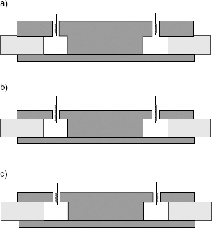
Figure 8.18 Relationship between coil length and magnetic gap length. a) Short-coil/long-gap. b) Long-coil/short-gap. c) Equal coil/gap length
Figure 8.18 shows three types of magnetic gap and coil proportions which can be used for low frequency drivers. Example a) shows a short-coil – long-gap design. This concept is perhaps the best for low distortion reproduction, because the coil remains in the gap and crossing the same number of flux lines throughout its range of travel. It is also apparent that the coil is in good thermal proximity with the large magnet assembly, so it can easily lose the heat which its resistance dissipates. The drawback to this design is predominantly cost, because of the large quantities of magnetic materials which are needed. Example b) shows the opposite approach, the long-coil – short-gap design. In this case, half of the coil is outside of the gap at any one time during its entire range of movement. This is good in terms of linearity of motion with drive signal, but it is bad in terms of efficiency and heat loss from the voice coil. The efficiency is poor because only a proportion of the energy put into the coil is acting on the magnetic flux lines crossing the gap, due to the fact that much of the coil always remains out of the magnetic gap. It is poor in terms of heat dissipation both because only half of the coil is surrounded by metal, to conduct the heat away, and, compared to the design shown in a), because there is less metal to do the conducting. However, less magnetic materials are used, so cost of production can be considerably reduced. In the cases of examples a) and b) the linearity can be excellent, but example a) tends to have the slight advantage.
In example c) the coil and gap are the same length. Production costs can be kept low, and efficiency can be kept high, but it can be appreciated that almost as soon as the coil begins to move, it begins to leave the gap. Once it begins to move out of the gap, less turns of the coil are influenced directly by the magnetic flux lines crossing the gap, although the fringing effect which extends beyond the gap will ameliorate the effect of the abrupt movement out of the gap. The result of this motion is that as more current is applied to the coil, it has less proportional effect as a driving force. The driving force is therefore not linear in its relationship to the drive current, so the acoustic output will be compressed in relation to the electrical input, and harmonic distortion will also be generated. For high quality music reproduction these effects would be disastrous, but they can be highly desirable in their effect on the sound of electric or electronic musical instruments, and even some amplified acoustic instruments, blues harmonica being one obvious example.
It is also essential in the design and construction of loudspeakers for high fidelity sound reproduction that the cones behave as closely as possible to pure pistons, or that any break-up which does exist decouples sections of the cone in order to control the directivity at higher frequencies. Normally, for high fidelity drive units, either strong, heavy, straight sided cones are used (where the weight is also useful for lowering the resonant frequency), or deep profile cone shapes can be applied. If more sensitivity and an extended high frequency response are required, a lighter weight curvilinear cone shape can be employed. These forms are as shown in Figure 8.19. The latter shape facilitates the decoupling of the outer regions of the cone at high frequencies, leaving the central area and the dome as the principle radiating areas, thus improving the control of the directivity whilst still preventing the break-up modes from circulating around the cone. At low frequencies, a straight sided, light-weight, shallow angle cone would not be desirable for high fidelity use, because it would lack the stiffness to act as a good piston. However, a straight sided, light-weight cone may be exactly appropriate for some musical instruments, where the extra sensitivity gives more volume per watt of amplifier power, and the colouration from the reduced stiffness can enhance the tonal response. Cone depth (apex angle) can also be chosen to move resonances into desirable regions. Light, shallow cones can exhibit rising, peaky, mid-range responses, which can be excellent for electric guitar amplification, despite being awful for high fidelity purposes.
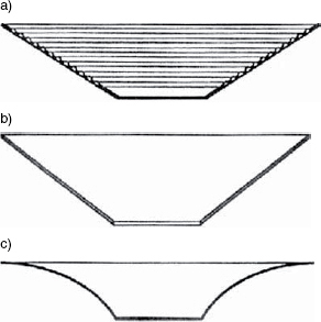
Figure 8.19 Cone profiles – they each serve best for different purposes. a) Ribbed, straight-sided – thickness and ribbing employed to increase rigidity. b) Deep, straight-sided – smaller apex angle employed to increase rigidity. c) Curvilinear – curved profile employed to aid decoupling of outer region of cone
What is more, high fidelity loudspeakers are generally intended to be used ‘sensibly’, but musical instrument loudspeakers may be purposely overloaded on many occasions to achieve certain sounds. For this reason, the suspension systems, as well as the voice-coil/magnetic-gap designs, may be used to limit the cone movements and offer some degree of self-protection from overload. Inevitably, this means the use of nonlinear suspensions, which add characteristic sound qualities that would be impossible to accept in a world of high fidelity, yet they may also add further characteristic tone qualities of a desirable nature to a musical instrument loudspeaker. In fact, once all of these ‘defects’ have come together in the right balance of qualities and quantities to produce their own, classic sounds, it can be very difficult for the drive unit designers to ‘improve’ the construction without losing the magic sound. Their sound can be something very difficult to define in technical terms, but the musicians can recognise even the slightest change from the original item. The Celestion company, for example, who produced 12 inch loudspeakers for the classic Vox (blue chassis) and Marshall (silver chassis) guitar amplifiers of the 1960s have had to find sources of exactly the same materials in order to make the same loudspeakers 40 years later. No amount of research and engineering or computer analysis has been able to achieve the same sounds from different designs. Conversely, their current high fidelity products are considered to be much superior to their products of the 1960 and 1970s, and none of the older designs remain in production.
8.6.1 Cabinet designs
In the glory days of amateur high fidelity, when almost all recordings were in mono, an enormous quantity of ‘patent’ cabinet designs were written about. Before the advent of stereo gave a whole new dimension to the spaciousness of the reproduction, many strange loudspeaker designs were offered in an attempt to bring more life to the reproduction, and to generally enhance the sensation of ‘being there’. Clearly, by the very fact that they were designed to enhance the reproduction, they could not, strictly speaking, be called high fidelity, but many of the designers claimed otherwise. Their point of view was that if the designs gave a greater sensation of being at the performance, then that in itself was a greater fidelity to the overall musical experience, even if it was not provable by objective measurement. The fact that many, current, portable music players have ‘stereo enhance’ and ‘super maxi bass’ facilities on them would seem to prove their case, at least when listening for pure pleasure is the goal, and when the basic reproduction is not the best that hi-fi stereo can offer. And it must also be said that many, modern, domestic surround systems are more likely to produce a pleasant sensation rather than anything which could be claimed to be a lifelike reality.
As stereophonic domestic music reproduction began to reach much better standards, in the late 1960s, many of the eccentric designs which had previously been offered began to disappear. In stereo, where the spacial enhancement was much less necessary, the strange designs only proved to be sources of annoying colouration, and the fact that they were not capable of producing true high fidelity became very apparent. However, not long after they had begun to fade from the hi-fi scene, some of them, such as the Karlson Coupler, from the 1950s, shown in Figure 8.20, began to be re-discovered by the makers of musical instrument amplifiers. In this new guise, where the concept of fidelity did not exist, the strange cabinets could freely and justifiably contribute their special sound enhancement characteristics to the realm of sound production. The original claim for the Karlson enclosure was that it de-tuned the normal resonance of the rear radiation path, making it responsive over a broad band, but objective measurement could largely only show that it produced response irregularities, and little else. It was also recommended for use with full-range loudspeakers, but it is hard to see how severe colouration could be avoided due to resonances and reflexions in the cavity in front of the drive unit. It is unimaginable to be listening to modern day CDs via such an absurd ‘design’, yet in the 1970s it made a big come-back as a popular and successful bass guitar loudspeaker, where its own sound was deemed to be very favourable, and such enclosures continue to be used to this day for instrument amplifiers.
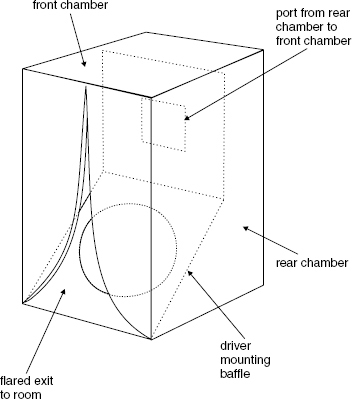
Figure 8.20 The Karlson Coupler, from the early 1950s
It is therefore very difficult to give specific guidelines for the design of cabinets for musical instrument amplification, because what sounds good is good; although it might be good for some players and their particular instruments but not good for others. It is also difficult to give target responses for overall performance, because good musical sounds, at their production stage, do not follow many set rules. Designers may well also break the accepted hi-fi standards when it comes to wiring the drive units in the cabinets, such as wiring woofers in series, specifically to reduce the damping and enhance the resonances and colouration. This idea may be further extended by using valve amplifiers without any negative feedback on the output stage. This raises the output impedance, and reduces the damping still further. Undersized output transformers may also be employed, to give rise to saturation and ‘overdrive’ effects at high levels. In fact, guitar amplifiers and loudspeakers are crafted more by artistry than by science, but so is the music which they help to create.
Summary
The recording chain from the musicians to the music buying public consists of five very different links. At each stage, the demands on the loudspeakers are different, and even if a perfect loudspeaker did exist, the circumstances of its application would render it non-optimal in many situations where specialised needs exist. Although the fundamental requirements are the same for the reproduction loudspeakers, the specific balance of characteristics can change to quite a large degree—very much so in terms of physical size. However, once we enter the world of musical instrument amplification, many of even the fundamental requirements change drastically, and what can be an absolute taboo for reproduction can be highly desirable for sound production, such as using 12 inch (300 mm) loudspeakers up to 6 or 7 kHz, for example. This not only goes for the loudspeaker drive units themselves, but also for the cabinets, the wiring, and the design of the amplifier output stages.
References
1 Newell, P., ‘Recording Studio Design’, Appendix 1, Focal Press, Oxford, UK (2003)
2 Walker, R., ‘The Selection of Loudspeakers for BBC Radio & Music’, Proceedings of the Institute of Acoustics, Vol 26, Part 8, pp 93-106, Reproduced Sound 20 conference, Oxford, UK (2004)
Bibliography
1 Colloms, M., ‘High Performance Loudspeakers’, 6th Edition, John Wiley & Sons, Chichester, UK (2005)
2 Fletcher, H., Munson, W.A., ‘Loudness: Its Definition, Measurement and Calculation’, Journal of the Acoustical Society of America, Vol 5, p 82, (October 1933)
3 Robinson, D.W., Dadson, R.S., ‘A Redetermination of the Equal-Loudness Relations for Pure tones’, Journal of Applied Physics, Vol 7, p 156, UK (May 1956)
4 ISO226, ‘Normal Equal-Loudness Level Contours’, International Standards Organisation, (1987)