
Chapter 11
Low frequency and transient response dilemmas
11.1 The great low frequency deception
Recording industry publications often contain advertisements proclaiming the true and lifelike responses of ‘accurate’ small monitor systems. If only from the sheer quantity of such advertising, it is entirely reasonable that many people would be led to believe that accurate low frequency reproduction from small boxes at quite high monitoring levels was an easily achievable goal, but the reality is rather different. At realistic listening levels for recording studio or mastering use, the low frequency response of small loudspeakers cannot be as accurate in terms of frequency response and transient response as that of a good large system, flush mounted in the front wall of a well-controlled room. The laws of physics simply will not allow it.
Various techniques can be used to flatten and extend the low frequency pressure amplitude of loudspeakers in small-to-medium-sized cabinets, but what so many people are unaware of is the degree to which these methods of response extension can distort the time responses of the systems, and mask considerable amounts of the low-level detail which a complex musical signal may contain. The magnitude of the problem is clearly depicted in Figure 11.1, from which it can be seen that of the 38 specimens tested, when the time, frequency and pressure responses are viewed together, no two out of the 38 plots look the same. It can also be added, without fear of contradiction, that no two loudspeakers sound the same, either. Using these loudspeakers as monitoring references therefore is more a question of interpretation rather than anything absolute.
The variability between these ‘reference’ loudspeakers is made all the more alarming when one considers two further points. Firstly, that all the measurements shown in Figure 11.1 were made in the same position in the same, large (611 m3) anechoic chamber. Obviously, when one uses these loudspeakers in typical control rooms or domestic rooms, the responses will be further adulterated. Secondly, it must be appreciated that amongst the 38 examples are some very fine loudspeakers, in fact all were submitted for test by manufacturers who were proud of what they had achieved, and all were presented as professional music-monitoring loudspeakers. Therefore, as these loudspeakers represent ‘the higher end’ of loudspeaker production, it is lamentable to think how poor the responses can be at the lower end of the market. Furthermore, it should also be obvious that if these plots represent the best that such famous manufacturers can do, then we are not dealing with any problems that can be easily solved. So, perhaps we should now look at the implication of what the plots represent, and analyse the problems step by step.
11.1.1 The air spring
Moving coil loudspeakers in boxes are volume-velocity sources. The acoustic output is the product of the area and the velocity of the diaphragm, so, for any given output, either a large volume of air can be moved slowly, or a small volume of air can be moved quickly. Let us say that, for a given SPL, the diaphragm of a 15 inch (380 mm) woofer in a 500 litre box moved 2 mm peak to peak. With an effective diaphragm radius of 61/2 inches, which is about 160 mm, (we do not count the surrounds as part of the radiating area), the radiation area would be 80,000 mm2. Moving 2 mm peak to peak means moving 1 mm from rest to the peak in either direction, so the unidirectional displacement would be 80,000 × 1mm3 or 80,000 mm3. This is equal to 0.08 litres, so the static pressure in a 500 litre box would be compressed (if the cone went inwards) by 0.08 litres, or by one part in 6250 of the original volume.
For the same SPL, a 6 inch (150mm) loudspeaker in a 10 litre box would still need to move the same amount of air 80,000 m3. However, with an effective piston radius of only 21/2 inches, or 65 mm, the cone travel would need to be about 12 mm peak to peak, or 6 mm in either direction, so it would also need to travel six times faster than the cone of the 15 inch loudspeaker, (i.e. 6 mm instead of 1 mm in the same period of time for any given frequency). What is more, the displacement of 80,000mm3 (0.08 litres) in a box of only ten litres would represent a pressure change in the box of one part in 125 of the original volume, compared to one part in 6250 in the 500 litre box. The air compression inside the box would therefore be 50 times greater than that in the 500 litre box, and there are several consequences of these differences.
Anybody who has tried to compress the air in a bicycle pump with their finger over the outlet will realise that air makes an effective spring. They will also realise that the more the air is compressed, the more it resists the applied force, and the bicycle pump can rarely be compressed much more than about half way. The force needed to compress the air by each subsequent cubic centimetre increases with the compression, so the process is not linear. In the case of the 15 inch and 61/2 inch cones referred to above, the cone in the small box would have a much harder job to compress the air by 1/125th of its volume than the cone in the large box, which only needs to compress the air by 1/6250th part in our previous example. (Cone size is irrelevant, here – only the volume displacement matters.) Large boxes therefore tend to produce lower distortion at low frequencies, because the non-linear air compression is proportionally less. The concept is shown diagrammatically in Figure 11.2.
The non-linearity of the air spring can perhaps also be better understood when one considers that it would take an infinite force to compress 1 litre of air to zero volume, yet it would take only a moderate force in the opposite direction to rarefy it to 2 litres. The forces needed for a given change in air volume in each direction (in this case ±1 litre) are thus not equal, so the restoring forces applied by the air on the compression and rarefaction half cycles of the cone movement are also not equal. The non-linear air-spring forces thus vary not only with the degree of displacement, but also with the direction of the displacement. Changing air temperatures inside the boxes also add more complications of their own, and waste-heat from the voice coils when the loudspeakers are being driven by a musical signal ensures that the temperature of the air will change during use. Therefore, for any given SPL, loudspeakers in small boxes tend to produce more distortion than similar loudspeakers in larger boxes.
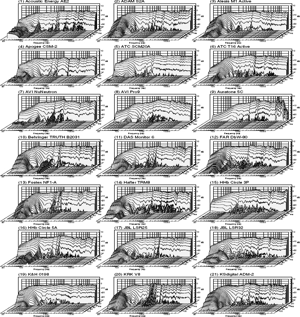
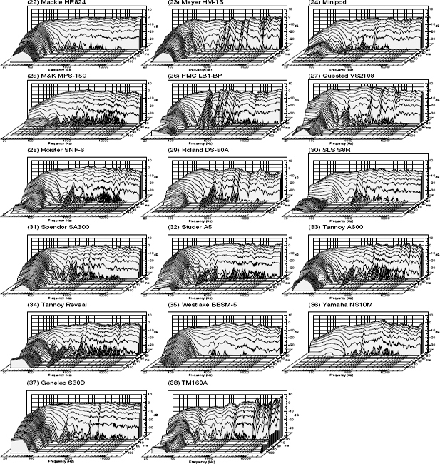
Figure 11.1 Waterfall plots of the anechoic responses of 38 loudspeakers
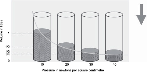
Figure 11.2 Boyle's law
Each pressure change of 10 newtons produces progressively less change in the volume of the gas. The process is therefore not linear, and can give rise to harmonic distortion
From this it can be seen that the more that a gas is compressed, the more it will resist further compression. The line passing through the cylinders is a curve, not a straight line, and this gives rise to the non-linear distortion (principally harmonic distortion) due to the back-loading on the diaphragm of a low frequency driver. In a big box, the relative compression is less, so for any given displacement the non-linear distortion due to the effect of the air spring will also be less
11.1.2 Size, weight and sensitivity
The main controlling factor for the extension of the low frequency response of a loudspeaker system is its resonant frequency, because the low frequency response of any conventional loudspeaker system will begin to fall off quite rapidly below the resonant frequency. There are systems which drive the loudspeakers well below resonance, with the application of electronic compensation, but they can run into problems of cone excursion limitations, and are not in widespread use. The resonance is a function of the stiffness of the air spring formed by the air inside the box, coupled with the moving mass of the loudspeaker cone/coil assembly. The fact that the air inside a small box presents a stiffer spring than the air in a larger box, (because it is proportionally compressed more for any given volume displacement) means that it will raise the resonant frequency of any driver mounted in it, compared to the same driver in a larger box (i.e. loaded by a softer spring). The only way to counter this effect, and to lower the resonant frequency to that of the same driver in a larger box, is to increase the mass of the cone/coil assembly. [Imagine a guitar string; if it is tightened, the pitch will increase. Maintaining the same tension, the only way to lower the note is to thicken the string, i.e. make it heavier.]
The problem that one now encounters is that to move the heavier cone, in order to displace it by the same amount as a lighter cone in a larger box, more work must be done, so more power will be needed from the amplifier. The sensitivity of a heavy cone in a small box is therefore less (for the same resonant frequency and bass extension) than for a lighter cone in a larger box. If the sensitivity is to be maintained in a smaller box, by using the same weight of cone and coil, then inevitably the resonant frequency will be forced upwards. So, as the box size decreases, either the bass extension or the sensitivity (or both) will be reduced. The only way to maintain the bass extension and the sensitivity is to increase the size of the box or the size of the magnets.
Larger boxes often tend to use larger drive units. A large diaphragm will tend to be heavier than a smaller one, and the large diaphragm may also need to be heavier to maintain its rigidity, as discussed in Section 7.2.2. This would suggest a lower sensitivity in free air, but larger drive units often also have larger magnet systems, which can easily restore the sensitivity, and a larger radiating area, in itself, increased the radiation efficiency, as was discussed in Section 7.2.2. Nevertheless, in small boxes, the greater pressure changes may require stiffer, heavier cones, in order not to deform under high pressure loads, so the efficiency can again be caused to reduce. Once more, a bigger magnet could be an answer, but it may not be a simple task to use a bigger magnet because it could seriously obstruct the free air movement behind the cone, and it could reduce the internal volume of the box, hence further stiffening the spring and again raising the resonant frequency, which could only be offset by making the cone assembly even heavier. If this were the case, the extra weight of the cone would have to be compensated for by using more power to drive it, and because putting in more power means that it would probably need a bigger (and heavier) voice coil to take the extra power, it could therefore need even more power to restore the output. So, now it should be becoming obvious that there are just so many things which conspire against the extended low-frequency performance of small boxes. There is no way out – we just keep going round in circles.
Let us now consider two actual loudspeakers of similar frequency range but very different size. A small loudspeaker such a the ATC SCM10 would need to be driven by almost 200 watts in order to give the same SPL at one metre as the double 15 inch (380 mm) woofered UREI 815 receiving one watt of input. The two loudspeakers are shown in Figure 8.11. As has just been discussed, reducing the box size demands that either the low frequency response will be reduced, or the sensitivity will be reduced. High sensitivity and good low frequency extension can only be achieved in large boxes. If the ATC seeks to achieve a good low frequency extension in a small box, then the sensitivity must be low; the air-spring physics dictates that this must be so. The ATC SCM10 has a box volume of about 10 litres; the UREI 815 contains almost 500 litres. Given that they cover the same frequency range, the sensitivity difference of about 22 dB is the result – hence the ATC needing almost 200 watts to sound as loud as the UREI receiving one watt.
11.1.3 Further consequences of small size
When small cones move far and fast, they also tend to produce more Doppler distortion (or frequency modulation), and this problem is often exacerbated by the small woofers being used up to higher frequencies than the large woofers, which can make the Doppler distortion more noticeable. The high frequencies are being radiated from a diaphragm which is moving backwards and forwards with the low frequency signals. (For more about Doppler distortion see the Glossary.)
Long cone excursions also mean more movement in the cone suspension systems (the surrounds and the spiders), which also tend to be non-linear in nature as cone excursions increase. That is, the restoring forces are rarely uniform with distance travelled. This tends to give rise to higher levels of intermodulation and harmonic distortion than would be experienced from larger cones of similar quality, moving over shorter distances. The larger movements also require greater movement through the static magnetic field of the magnet system, which tends to give rise to greater flux distortion and, even more audible, non-linear Bl profile distortions.
Furthermore, the reduced sensitivity of the smaller boxes means that more heat is expended in the voice coils compared to that produced in the voice coils of larger loudspeakers for the same output SPLs. This problem is even further aggravated by the fact that the smaller loudspeakers have greater problems in dissipating the heat, because there is less air surrounding them in the smaller boxes. This can lead to thermal compression, as the hotter the voice coil gets, the more its resistance increases, so the less power it can draw from the amplifier for any given output voltage. The resulting power compression produces yet more distortion products, so it can clearly be seen that the distortion mechanisms acting on small loudspeakers are far greater than those acting on similarly engineered large loudspeakers. And even that is not all; small cones rapidly punching thought the air can produce turbulence, which can be a source of strange noises due to the shearing of the air at the edges of the cone. There are thus many reasons why large-coned drivers moving over short distances tend to produce less distortion than smaller ones, of similar quality, moving over larger distances. All of these reasons militate against the low frequency performance of small loudspeakers.
11.2 Commercial solutions
The commercial pressures on loudspeaker manufactures tend to come from people who are largely ignorant of these problems. The typical customers demand more output of a wider bandwidth from ever smaller boxes, so loudspeaker manufactures try to rise to the challenge. One example of a technique used to augment the low frequency output is to use a reflex loaded cabinet, (as described in Chapter 3) with one or more tuning ports. In these systems, the mass of air inside the ports resonates with the spring which is created by the air trapped within the cabinet. If the resonant frequency is chosen to be just below where the driver response begins to roll-off, then the overall response can be extended. The resonance in the tuning ports begins to radiate sound just where the drivers begins to lose their output, and so the overall response can be extended downwards.
The effective extension of the low frequency response by means of reflex loading also increases the loading on the rear of the driver as resonance is approached. This helps to limit the cone movement and to protect the drivers from overload. Unfortunately though, once the frequencies pass below resonance, the air merely pumps in and out through the ports, and all control of the cone movement is lost. In many active monitor systems, electrical high-pass filters are used to sharply reduce the input power to the drivers at frequencies below the cabinet resonance frequency. This enables higher acoustic output from the loudspeaker systems within their intended bandwidth of use, without the risk of overload and mechanical failure due to high levels of programme below the resonance. By such means, a flat pressure amplitude response can be obtained to a lower frequency than with a sealed box of the same size, and the maximum SPL can be increased (typically 3–4 dB for similar sized boxes) without risking drive unit failure, but there is a price to be paid for these gains. The phase response will be compromised, and hence the uniformity of the time (transient) response will tend to be lost.
11.2.1 The time penalty
It must be understood that a resonant system can neither start nor stop instantly. The time response of reflex loaded loudspeakers therefore tends to be longer than that of similar sealed box versions, which means that transients will be smeared in time: the impulse response will be longer. Moreover, the effect of the electrical high-pass filters is to further extend the impulse response, because the electrical filters are also resonant (tuned) circuits. In general, the steeper the filter slope for any given frequency, the longer it will ring. More effective protection therefore tends to lead to greater transient smearing. Figure 11.3 shows the low frequency decay of a sealed box loudspeaker, with its attendant low frequency roll off. Figure 11.4 shows the low frequency response of an electrically protected reflex cabinet of somewhat similar size. Clearly the response shown in Figure 11.4 is flatter until a lower frequency, but a flat frequency response is not the be-all and end-all of loudspeaker performance. Note how the response between 20 Hz and 100 Hz has been caused to ring on, long after the higher frequencies have decayed.
Figure 11.5 shows the corresponding step-function responses, and Figure 11.6 the acoustic source plots. These plots clearly show the time response of the reflex cabinets to be significantly inferior to the sealed boxes. The low frequencies from the reflex enclosure arrive later (as can be seen from Figure 11.6), and take longer to decay (as can be seen from the decay tails in Figure 11.5), which both compromise the ‘punch’ in the low frequency sound. Figure 11.7 compares the two plots of Figure 11.6 with the acoustic source plot of a large, wide-band, flush-mounted studio loudspeaker system in a well-controlled room. From this comparison it should be obvious why the NS10M (and Auratone 5C before it) earned a reputation as a punchy little ‘big’ monitor.
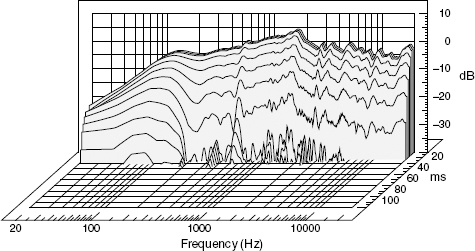
Figure 11.3 Waterfall plot of a small, sealed-box loudspeaker (NS10M)
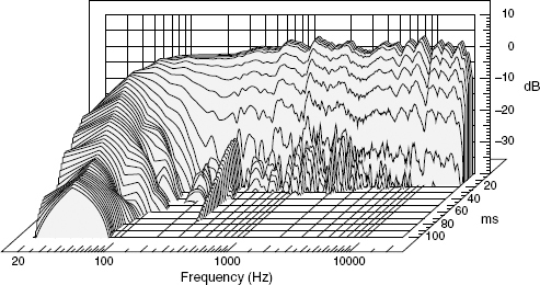
Figure 11.4 Waterfall plot of a small reflex (ported) enclosure of similar size to the loudspeaker whose response is shown in Figure 11.3
A sealed box cabinet will exhibit a 12 dB per octave roll-off below resonance, but a reflex enclosure will exhibit a 24 dB per octave roll-off when the port output becomes out of phase with the driver output. As the system roll-offs are often further steepened by the addition of electrical protection filters below the system resonance, sixth, and even eighth order roll-offs (36 dB and 48 dB per octave, respectively) are quite common. With such protection, some small systems can produce high output SPLs at relatively low frequencies, but the time (i.e. transient) accuracy of the responses may be very poor. We will return to this topic in the next sections of this chapter.
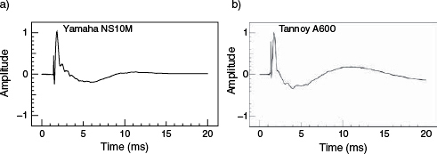
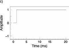
Figure 11.5 Step function responses corresponding to the waterfall plots shown in Figures 11.3 and 11.4, compared to the electrical input signal shown in (c). Note how rapidly the NS10 (a) returns to a flat line on the zero amplitude level
Inevitably, the different resonances of the different systems will produce musical colourations of different characters. This may not be a serious problem for use in domestic listening, but such inconsistency of colouration does little to help the confidence of the users in recording studios. If a mix sounds different when played on each system, then how does one know which loudspeaker is most right, or when the musical balance of the mix is correct? The resonances of the sealed boxes tend to be better controlled, and are usually much more highly damped than their reflex-loaded counterparts. This leaves the magnitude of the frequency response of sealed boxes as their predominating audible characteristic, but it is usually the time responses of reflex enclosures (related to the ‘phase’ part of the frequency response) which give rise to their different sonic characters. There is considerable evidence to suggest that the many years of use of the Auratone 5C and Yamaha NS10Ms as mixing monitors has been due to their rapid response decays. It can be seen from their response plots (Numbers 9 and 36 in Figure 11.1) that all the frequencies decay at an equal rate – none can be seen to be hanging on after the other frequencies have disappeared.
A simple roll-off in the low frequency response of a loudspeaker used for mixing is in itself not a great problem, because any wrong decisions about a balance can usually be corrected by equalisation at a later date, such as during mastering. As previously stated in other chapters, an error in the time response, such as that added by tuning port and filter resonances, can lead to misjudgements especially between the percussive and tonal low frequency instruments, such as bass drums and bass guitars, whose relative levels cannot be adjusted once they have been mixed together. The time response errors of the loudspeakers will have led to erroneous mixing decisions which cannot be unscrambled. The concept will be treated in a more definitive manner in Section 11.7.
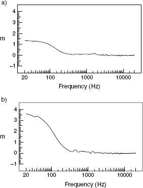
Figure 11.6 Acoustic source plots corresponding to the waterfall plots shown in Figures 11.3 and 11.4
In these plots the low frequency response delay is shown in terms of from how many metres behind the loudspeakers the low frequencies are apparently emanating. As each metre corresponds to about 3 milliseconds, it can be appreciated how the low frequencies from behind the sealed box (a) arrive much more ‘tightly’ with the rest of the frequencies than they do in the case from the reflex cabinet
11.2.2 The transient trade-off
A problem therefore exits in terms of how we can achieve flat, uncoloured, wide-band listening at relatively high sound pressure levels from ten-litre boxes. At the moment, basically, the answer is that we cannot do it. Just as there is a trade-off between low frequency extension, low frequency sensitivity/efficiency (see Glossary) and box size; there is also a trade-off between low frequency SPL, bass extension, and transient accuracy if bass reflex loading and electrical protection are resorted to in an attempt to defeat the box size limitations. In effect, the bass extension is gained at the expense of transient accuracy.
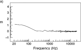
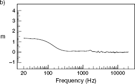
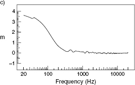
Figure 11.7 Acoustic source plots of Figure 11.6 compared to the acoustic source plot of a large, flush-mounted, studio monitor loudspeaker. a) A 700 L, wide-range, flush-mounted studio monitor loudspeaker. b) A Yamaha NS10M. c) A popular, small, reflex-loaded, close-field loudspeaker system. Note how the response of the NS10M mimics that of the large monitor loudspeaker system. There is therefore little wonder that the NS10M has a reputation for having a ‘rock and roll punch’
We therefore have a state of affairs whereby, at low SPLs, good low frequency extension can be achieved from small boxes, but the non-linearity of the internal air-spring can lead to high distortion when the cone excursions, and hence the high degrees of internal pressure changes, become significant. Suspension and magnet system non-linearities can add further problems, and remember also that in a small box there often exists the problem of how to get rid of the heat from the voice coil. Thermal overload and burnout are always a problem at high SPLs due to the high power necessary to overcome the limitations of the poor system efficiency. Larger, higher-sensitivity systems not only produce less heat for any given SPL, but also are much better at dissipating it. They thus win on both counts.
From the waterfall plots of Figures 11.3 and 11.4 it can be seen that, whatever the box type, the decay is never instantaneous. There is always a slope to the time representation, which in these plots is depicted by the time ‘slices’. One can imagine the slope of the plot in Figure 11.3 continuing below the ‘floor’ formed by the frequency and time axes, with the lines of the ‘waterfall’ continuing to cascade down. The question has often been asked whether the electrical flattening of the low frequency response would inevitably lengthen the time response, even with the sealed boxes – effectively extending the response on the time scale as the level was brought up from below the ‘floor’ on the amplitude (vertical) scale. In truth, the tendency is for the flattening of the amplitude response to shorten the time response (i.e. steepen the slope) by means of its correction of the phase response errors which are associated with the roll-off. This means that a large or small sealed box, equalised or not, would still exhibit a much faster time response than a reflex enclosure. Figure 11.8 shows the comparative effect.
Unfortunately, the type of equalisation shown in Figure 11.8 is not a practical option, because even at very low sound pressure levels, the excursion limits of a small drive unit would be exceeded at the lowest frequencies, and the drive-power levels would double every time that an extra 3 dB of boost was applied. Figure 11.8 only serves to show how, in principle, corrective equalisation would beneficial to the entire time/frequency/phase response.
It seems reasonable that the more extended bass response of reflex enclosures may well be valuable to ‘vibe’ the musicians during the recording process, where concentration is more on achieving a good performance rather than necessarily looking at the subtleties of each sound. However, during the mixing process, another, more critical view is required, and hence perhaps a different set of loudspeakers. At the mastering stage, the requirements for sonic transparency can become even more critical, and hence we have arrived at the sort of differentiation of uses described at length in Chapter 8.
There are those who say that very fast time responses are not necessary from loudspeakers, because their decay times are considerably shorter than many of the rooms in which most of them will be used. However, what they fail to realise is that the small loudspeakers are usually being used in the close-field, which is normally considered to be within the critical distance where the direct sound and room sound are equal in level. It therefore follows that if one is listening in the close-field, the responses of the loudspeakers will predominate in the total response. Indeed, this is one of the principal reasons for the use of close-field listening. The room decay will therefore not totally mask the loudspeaker decay, except in rooms which are so live that the close field extends only a matter of centimetres from the loudspeakers, but such rooms would hardly be appropriate for monitoring.
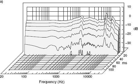
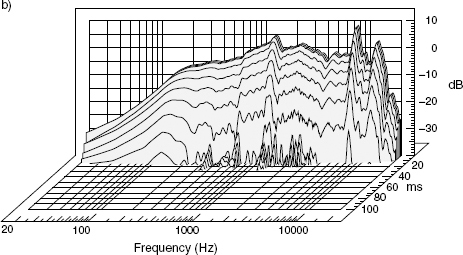
Figure 11.8 Time vs. frequency – the effect of equalisation on a sealed box loudspeaker. a) Waterfall plot showing the effect on the time response of electrically flattening the response of an Auratone 5C. Although the response is now flatter down to a lower frequency than the reflex enclosure shown in Figure 11.4, the time response has not been extended – the decay is much more rapid. Unfortunately, such equalisation is not a practical solution because the loudspeaker would overload even at low SPLs. Compare this plot with the unequalised response shown in (b), from which it can be seen that the time response has not been lengthened in the slightest by the corrective equalisation
11.3 The evolution of the desk-top monitor
It came as a bit of a shock during interviews with some highly respected recording personal to find not only how little they knew about loudspeakers, but also how little they cared about knowing what was going on inside the boxes. They seemed only to be interested in whether they worked, or not, for their own decision-making during recording or mixing sessions. In effect, it seems that they have largely given up trying to understand a subject which usually appears to be cloaked in so much mystery. The problem with this is that it provides very little feedback to the loudspeaker designers, and the trend towards aggressive marketing of the products also does little to increase the breadth of understanding of the users.
Somewhat disturbingly, even the designers of many professional loudspeaker system are under the influence of powerful marketing pressures. When they receive instructions from their paymasters to design a new loudspeaker, sound quality can be as low as fourth or fifth on the list of design priorities. Things such as to be 100 euros a pair cheaper than the perceived competition, an eye-catching design that will look good in advertisements, comparable size to a competitor, and to be louder than the nearest competing models are often typically seen to be more important than absolute sound quality by the largely all-powerful marketing/sales people, even in a supposedly professional recording industry.
However, despite this, mastering engineers, recording engineers, producers and musicians have been able to find some common paths, which, even if they have not been clearly marked by technical guidelines, have nevertheless been leaving some clear sonic footprints. Look, for example at Figure 11.9. How many users of Auratones and NS10s have ever realised that they possessed such similar frequency responses, (at least below 6 kHz) or how different their ‘inverted V’ anechoic frequency responses were from most other loudspeakers? The waterfall plots shown in Figure 11.10 (which show pressure amplitude against time against frequency) are also very similar, as are the step function responses shown in Figure 11.11. These plots help to explain why such a large number of recording engineers and producers moved to the NS10 as a louder and deeper replacement for their trusted Auratone 5Cs. The NS10 basically gave them more SPL and more bass than the Auratones, but the general characteristics of the sound remained the same. The reasons why only became apparent about 20 years after the switch had taken place by the judgement of ears, alone1.
The plots in Figure 11.9 are anechoic chamber responses, and it is clear that in the frequency domain they are not flat with frequency. Technically, they seem wrong, but sonically, at least for achieving a musical balance between instruments, many users find them to be right when used in their typical console-top locations, the effect of which on the pressure response was shown in Figure 8.12.
Let us consider the implications of Figure 8.12(a), shown again, here, as Figure 11.12. The solid line shows the predicted response of a loudspeaker such as an NS10M in a free-field (as in an anechoic chamber). The shape is not unlike the measured anechoic responses of the NS10M and the Auratone 5C, as were shown in Figure 11.9. The broken line shows the predicted response when such a loudspeaker is flush mounted in a wall. When one considers that the NS10M was originally designed as a bookshelf loudspeaker, the logic behind its anechoic response should now be clearly apparent. In fact, if sited next to any large reflective surface, such as the top surface of a large mixing console when placed on its meter bridge, the response would also tend towards that of the broken line. Figure 11.13 shows the actual response of an NS10M on a meter bridge in a typical recording environment. Obviously the desk (console) tops cause many response irregularities, but, the general tendency towards an overall response flatness is also very apparent in Figure 11.13. The low frequency response has clearly been augmented, and what is more it has been augmented in a non-resonant manner that does not affect the rate of decay of the low frequencies.
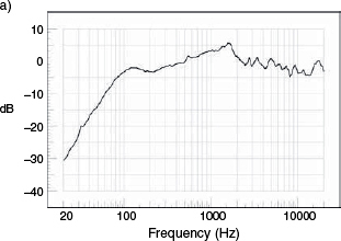
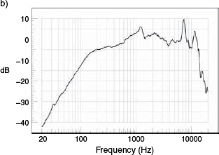
Figure 11.9 Comparisons of pressure amplitude responses of the NS10M and the Auratone 5C loudspeakers. a) NS10 anechoic frequency response plot. b) Auratone 5C anechoic frequency response plot. Note the general similarity of the frequency responses (apart from the peak at 8 kHz in the Auratone's response). The fact that they are not flat is also worthy of note
The great significance of this is that if a loudspeaker which had a flat anechoic response were to be similarly positioned, it would also be subjected to the same type of response modifications, and so would tend to produce an excess of low frequencies. This is the reason why many active loudspeakers have bass frequency adjustment switches, with recommended settings for different mounting conditions. With passively crossed-over loudspeakers, this flexibility in response correction is only usually achievable by the use of external equalisers, but it is seldom a practical solution. Low frequency response controls can be incorporated into an active design for a few cents, but a dedicated equaliser with the sonic transparency necessary for high quality monitoring may be vastly more expensive than the loudspeakers with which they are being used. This tends to discourage their use. Obviously, the use of a cheaper equaliser, with its own sonic character, would be an absurd choice if accurate monitoring were the goal. Passively crossed-over loudspeakers therefore tend to be best chosen with responses appropriate for their conditions of mounting, but a large proportion of the people involved in the recording world seem not to understand this rather important point.
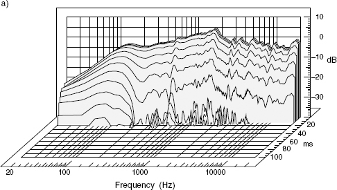
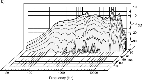
Figure 11.10 Comparison of the waterfall plots of the NS10M and the Auratone 5C loudspeakers. a) Waterfall plot of NS10M. b) Waterfall plot of Auratone 5C. By 20 milliseconds after the wideband excitation has ceased, the response at almost all frequencies has decayed below the −40 dB level. This is not the case with most small reflex loudspeakers, of which the plot of Figure 11.4 is more typical
The upshot of this is that loudspeakers get located in positions that are physically practical for working, but which may not be conducive to optimising the flatness of the low frequency response, and usually no measures are subsequently taken to correct the overall response. A small bookshelf loudspeaker, for example, will be acceptably flat, in wideband terms, when mounted on a meter bridge of a suitably sized mixing console, but the consequent comb-filtering due to the desk-top reflexions will reduce the sonic openness and transparency. (The effect of the reflexions can be seen in the irregularity of the response shown in Figure 11.13). These latter two aspects could be restored by positioning the loudspeakers behind the console, on pedestals, but then the low frequency reinforcement would be lost and the bass response would fall off more rapidly. Neither situation is therefore ideal. In the case of pedestal mounting, because the low frequency roll-off is a result of the lack of loading on the bass driver, it could be equalised by a suitably sonically neutral equaliser. [Note that this is not a room response problem, which could not be properly corrected by means of equalisation, but rather it is a loudspeaker air-loading problem, which can legitimately be equalised]. The equaliser would, in this case, correct the loudspeaker response in terms of both amplitude and phase, but unfortunately it would also reduce the headroom, so overloads would be likely at lower than normal volume levels. This is therefore not perceived to be a useful solution.
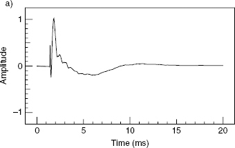
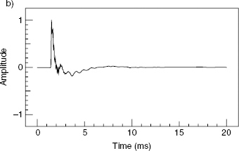
Figure 11.11 Comparison of the step-function responses of the NS10M and Auratone 5C loudspeakers. a) NS10M step function. b) Auratone 5C step function. By 8 milliseconds after the impulsive excitation, the responses have decayed to a flat line. Again, this is not typical of most loudspeakers of which, once again, the step-function response shown in Figure 11.5(b) is perhaps more typical
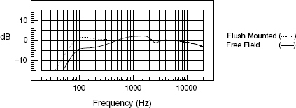
Figure 11.12 Response of an idealised loudspeaker, of similar size to an NS10M, under different conditions of mounting
The solid line shows the free-field response, and the dotted line shows the expected response if flush-mounted
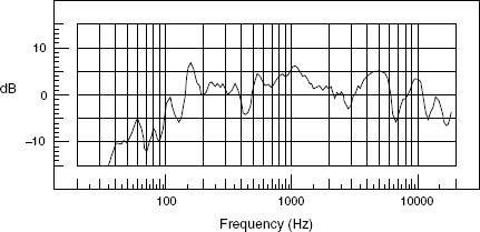
Figure 11.13 Response of a Yamaha NS10M loudspeaker on top of a mixing console meter bridge in a typical, small control room
Note the general tendency towards an overall flat response. The irregularities are desk-top reflexions, which would tend to similarly affect the responses of any loudspeakers so mounted
From this discussion it should be apparent that a loudspeaker mounted on the meter bridge of a mixing console, in a control room, could not be expected to perform similarly when placed on pedestals in a mastering room. So, this is one clear example of why mastering engineers may need different loudspeakers to the ones used in recording studios – they use them differently. What is more, it must be fully understood that loudspeakers which are to be mounted on pedestals tend to need a flatter anechoic low frequency response than loudspeakers which will be mounted in walls, next to walls, or on meter bridges. A loudspeaker with a fixed, passive crossover and with a flat anechoic frequency response is therefore not suitable for meter bridge mounting.
11.4 The great time deception
The problems discussed so far in this chapter would appear to be at the root of the frequent observation by mastering engineers that the recordings from the studios with less-experienced personnel frequently display incorrect balances between the bass instruments. If a loudspeaker exhibits a resonant low frequency response, it will add this resonance to the response of the instrumental sounds that it is reproducing. This may be of little significance to a resonant instrument like a bass guitar, but it may very distinctly alter the character of a tight, fast-decaying, percussive bass drum sound. The added resonant energy could mislead the mixing personnel into believing that the bass drum was louder in the mix than was actually the case. They would hence balance the instruments with the bass drum lower than it should be with respect to the bass guitar. When it comes to the mastering stage, little can be done to rectify the situation, because the equalisers or compressors usually cannot act on the bass drum without also acting on the bass guitar. The only solution may be to go back to the studio and do another mix with more bass drum, and incur whatever extra expenses and wasted time that may be involved.
Conversely, if a mix was done on loudspeakers with fast, low-frequency decays, albeit deficient in bass extention, the situation may not be so bad. If the instruments were balanced between themselves, a simple equalisation process (taking off whatever low frequency had been added due to the lack of bass on the mixing loudspeakers) could return the overall response to that which the recording staff thought that they had at the time of mixing. But it is the errors in the loudspeakers’ time responses which are the great deceivers in so many cases, and the mixing errors which they lead people to make are often unable to be corrected by any currently known signal processing device.
It still seems to be the case that too many loudspeaker manufactures who make products specifically aimed at the music recording market are paying too much attention to the flattening of the pressure amplitude of the frequency response and too little attention to the shortening of the time responses. This could, at least in part, be down to the fact that the anechoic response flatness sells loudspeakers by looking good in brochures, whereas a short time response does little to sell the loudspeakers because 99% + of the users are unaware that a time response problem even exists. This is a pity, because we now have the evidence available to show how important the fast decay of a time response is to the sonic neutrality of a system2.
11.5 Resonant tails and one-note bass
Figure 11.14 shows the frequency responses of ten different small loudspeakers, all ostensibly designed for use as small monitors in recording studios3. It can be seen how the responses below 200 Hz are all quite different. Numbers 1 and 2 are sealed boxes, which roll off naturally at 12 dB per octave. Number 1 is a larger box than Number 2, so it typically exhibits a flatter response to a lower frequency before the roll-off begins. The eight subsequent plots all show the responses of loudspeakers which have used different acoustic or electro-acoustic means to attempt to maintain the flatness of the response to lower frequencies than would be achievable if the boxes had been sealed. Number 10 exhibits a response not unlike Number 1, albeit with a steeper roll-off, but in a rather smaller box than that of Number 1.
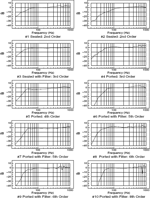
Figure 11.14 Low frequency responses of ten small, monitoring loudspeakers
Figure 11.15 shows another series of plots. These show the responses of six of the loudspeakers shown in Figure 11.14, but after excitation with a burst of four cycles of 60 Hz. The ‘order’ referred to in the captions below each of the plots relates to the overall rate of low frequency roll-off: each ‘order’ represents 6 dB per octave. Whilst there is nothing in Figure 11.14 to suggest that there could be any significant problem with the means that have been used to extend the flatness of the on-axis responses, Figure 11.15 begins to cast doubt on their validity. Note what happens as the box resonances are used to extend the low frequency flatness, and the electrical filters are applied in order to prevent over-excursion of the cones at frequencies below those of the box resonances. Number 1, a simple sealed box, shows a relatively straightforward decay at 60 Hz. But look at the ported enclosures, Numbers 5 and 7. The port tunings are not high Q, so their resonances are rather broad. This means that they can be excited by other frequencies which are reasonably close to their own resonant frequencies. The four cycles of 60 Hz are sufficient to excite the nearby port resonances, and it can be seen that as the 60 Hz excitation (at the top of the plots) decays, the electro-acoustical resonances continue to ring on. In effect, the decay of the excitation note shifts in frequency. In the cases of Numbers 8 and 9, double resonance can be seen to continue, with the initial excitation frequency bifurcating into separate resonant decays. If the excitation was a musical signal, then these resonances may not relate to the musical input. They may even be very discordant.
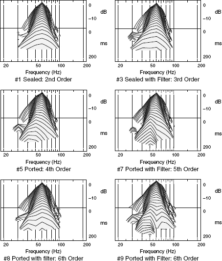
Figure 11.15 Waterfall plots of 4 cycles of a 60 Hz tone reproduced by six different loudspeakers
Of course, this can also happen in ‘boomy’ rooms, where room resonances are excited at frequencies nearby the original musical input. Some concert halls or performance stages are notorious for their ‘out of tune’ decays, which can be quite noticeable and undesirable during acoustic performances. In the cases of large, often multi-purpose rooms, the problems can be difficult to treat, due to the sheer, physical scale of the treatments, but in loudspeakers the problems are surely the result of either ignorance or inappropriate engineering design. Clean-sounding bass is hardly likely to be heard from loudspeakers which are generating their own low-frequency signatures.
11.6 The masking of detail
Another aspect of loudspeaker resonances is their tendency to mask detail in the signal. Figure 11.16 shows representations of the reproduction of a modulated noise signal. This was a pseudorandom noise with a bandwidth from 35 Hz to 70 Hz, modulated by a 10 Hz sine wave. The process was not unlike that which is used to measure speech intelligibility in voice evacuation systems (Speech Transmission Indices – STI and RASTI). In these plots, the shallower the modulation depth, the more the loudspeaker is likely to mask low frequency detail – or bass articulation as it may be referred to. The sealed box, with the second order roll-off, shows a modulation depth of around 32 dB (from 50 dB, down to 18 dB). The sealed box with an electrical protection filter (Number 3) reduces this to about 26 dB. By the time we get to the ported enclosure with the second order electrical protection filter, the modulation depth is down to about 14 dBs.
As the boxes become progressively more tuned and protected, the detail in low level signals can become progressively more lost. Once again, larger, sealed boxes perform much better.
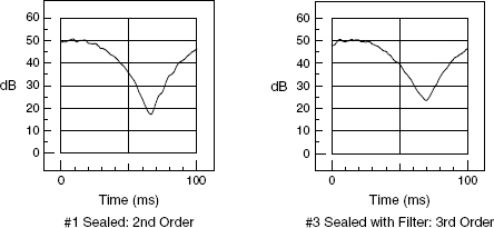
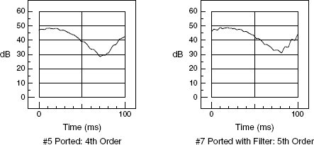
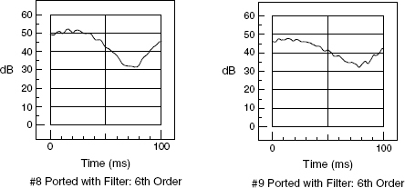
Figure 11.16 Averaged, convolved, modulated noise via six different loudspeakers
11.7 Theoretical equalisation and excess phase
Figure 11.17 shows the waterfall plots of the anechoic, on-axis responses of the same ten loudspeakers represented in Figure 11.14. They are all boxes of reasonably similar size. It can be seen that the low frequency resonances tend to increase in their decay time as the order of roll-off increases. Due to the general irregularity of the frequency responses, it is hard to accurately compare one response with another. Nevertheless, it should be easy to appreciate that each loudspeaker would be likely to lead mixing personnel to make different level and equalisation decisions with respect to the low frequency instruments in their musical mixes. So, in terms of references, they are clearly not compatible. The big question is, to what degree would the mixing misjudgements made on each loudspeaker be correctable?
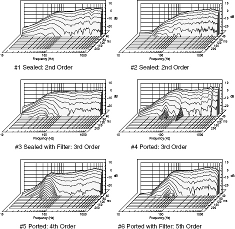
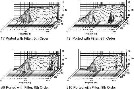
Figure 11.17 Waterfall plots of the same anechoic responses as shown in Figure 11.14
If people make different equalisation decisions at the mixing stage, then it should be possible to reverse them at the mastering stage if the decisions were global, that is, if extra bass was added to most low frequency instruments, or a little extra top was added. However, as was discussed in Section 11.4, if people have been led into equalisation or level decisions due to time response irregularities in the monitors, then those decisions are idiosyncratic to those monitors only, and may not relate well to the balance as heard in the mastering rooms. For the purposes of a research paper for a conference on acoustics, an attempt was made to ‘do what the mastering engineer would do’, by trying to equalise the response of the ten loudspeakers represented in Figure 11.17, and to try to see what was left in the response if they were all equalised to a common flatness3. Figure 11.18 shows that the results after the minimum phase portions of the frequency responses (the parts which are correctable in their phase responses as they are corrected in their amplitude responses) were ‘normalised’ by a digital computer. The idea behind this being that if all of the loudspeaker responses could be equalised to be flat, then the mixes done on all of them should subsequently be equalisable back to flat.
All of the upper traces of the ten plots shown in Figure 11.18 can be seen to be more or less equal, but the rates of decay have not been made uniform. Although the top line of the response of Number 3 is very similar to the top line of Number 8, the continuing resonance of loudspeaker Number 8 would undoubtedly lead to a more smeared, coloured, resonant sound in the bass response, and a probable perception of more bass, all due to time domain artefacts which have no solution in the frequency domain (i.e. by equalisers). No matter how flat the frequency responses of these loudspeakers can be made, the fact remains that their time response discrepancies would still lead to different mixing decisions. So, the implication, here, is that the loudspeakers which can be equalised flat in the frequency domain, without any significant hang-over in the time domain, should tend to lead mixing personnel into subsequently equalisable mixes. Judgemental errors made on loudspeakers which show resonant hangover, even after frequency response flattening, would tend to need to be re-mixed. In other words, given non-perfect loudspeakers, the ones which can be equalised closer to ‘perfection’ in both the time and frequency domains will tend to lead to more correctable mixes at the mastering stage.
11.8 Modulation transfer-function and a new type of frequency response plot
Fashions and marketing can have a huge influence on the loudspeaker buying public. This is especially worrying when the loudspeakers will not simply be used for the enjoyment of listening to music, but rather will be used, supposedly, to try to mix to some reference standard. If we don't use some at least reasonably standard conditions for music mixing, then what is there for a ‘high-fidelity’ domestic systems to be faithful to? In the Concise Oxford Dictionary, ‘fidelity’ is defined as ‘strict conformity to truth or fact; exact correspondence to the original’. But how can one conform in the home if the original sources of references are so variable? Taste, of course, comes in to this question, but so many of the tonal balance difference between music recordings in the shops are due to the wide variability of monitoring conditions. Something more revealing than the frequency response graphs has long been needed, and the MTF concept, introduced in Chapters 7 and 11, can be used to give much more insight into the potential sonic accuracy of different loudspeakers.
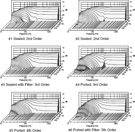
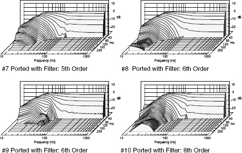
Figure 11.18 Waterfall plots of the excess-phase responses of the loudspeaker responses shown in Figure 11.17
Traditionally we have relied on the modulus of the frequency response (commonly referred to as simply the frequency response) as the standard of reference, but it should be clear from Figure 11.1 that even two loudspeakers with similar ‘top lines’ on the waterfall plots can hardly be expected to sound the same if the remainder of the decaying responses are so difference. Something more was needed to define the low frequency responses, so research was undertaken to try to adopt Speech Transmission Index (STI) techniques to look at the ability of loudspeakers to convey the full information content of the signals4. The STI is a means of calculating the voice modulation carrying the message through the general background noise. The idea proposed for the research was to use the concept of a typical modulation transfer function (MTF) calculation to determine how much detail could be carried on a low frequency signal without being blurred by resonances or distortions. To investigate this, the impulse responses of the loudspeakers were convolved with a modulated noise signal; a pseudo-random noise with a bandwidth of about 35 to 70 Hz, modulated by a 10 Hz sine wave. The results are shown in Figure 11.19, three of which are taken from the same group of results shown in Figure 11.16.
A sealed box exhibits a second order roll-off (12 dB/oct) below the resonant frequency of the system. Adding a first order, high-pass electrical protection filter yields a third order roll-off (18 dB/oct). A ported enclosure typically shows a fourth order (24 dB/oct) roll-off below resonance, and adding a second order protection filter results in a sixth order (36 dB/oct) roll-off. As can be seen from Figure 11.19, as the order of roll-off increases, the modulation depth reduces. In the cases shown, the depth varies from about 28 dB for the simple sealed box to only about 14 dB for the sixth order ported system. This indicates that bass detail is being lost in the ported systems, especially the ones with the added electrical protection filters. Nevertheless, although this shows what is happening, it still does not provide and easily describable accuracy measure. What was needed was a means by which to demonstrate not only the flatness of the response but also the accuracy with which the detail in the overall signal was being preserved.
Obviously, the modulation depth of the 20 to 30 Hz region of a loudspeaker whose response is already 40 dB down by those frequencies is not going to play much part in the subjective assessment of the sound, so a way had to be found to cross-correlate the modulation accuracy with the useful response of each system. A level of 85 dB SPL was chosen as a typical listening level, then the loudspeaker responses were convolved with an inverse of the minimal audible field curve (MAF) from the typical Robinson-Dadson curves for the sensitivity of human hearing – as shown in Figure 8.4 – similar to the well-known Fletcher-Munson curves. This yielded a compromise between response flatness and modulation accuracy. The plots of Figure 11.20 show the resultant MTF curves for the same four loudspeakers as in Figure 11.19. The MTF (vertical) scale is marked from 0 to 1. Zero would represent a response with no relation to the input signal, and 1 would represent perfect reproduction. The graphs are therefore plots of reproduction accuracy versus frequency. They are not frequency response plots; however, from them it can be seen which loudspeakers keep the highest MTF accuracy down to the lowest frequencies, so they are, in effect, low frequency quality response plots.
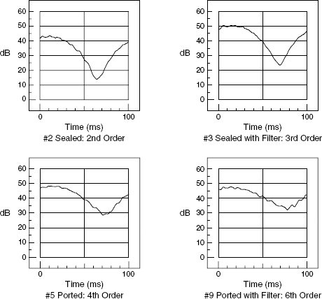
Figure 11.19 Averaged, convolved, modulated noise responses for the four example loudspeakers. It can be seen how as the order of low frequency roll-off increases, the modulation depth decreases. In other words, the information content in the signal decreases
Whilst the ‘frequency response’ plots of Figure 11.14 would suggest that the ported enclosure with the fourth order roll-off would be a much better monitor loudspeaker than the simple sealed box shown in plot Number 2, the plots of Figure 11.20 show that the small sealed box maintains a response accuracy, in terms of detail in the sound, down to a lower frequency than the fourth order ported box. In these plots, the total area below the curve is effectively a measure of response quality, whereas in Figure 11.14, the area below the curve only represents level; irrespective of whether that level is of anything connected with the music, or not, as shown by the extraneous resonant frequencies in Figure 11.15, which only serve to swamp the detail in the musical signal.
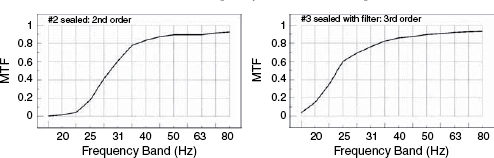
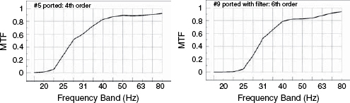
Figure 11.20 MTF results for the four example loudspeakers at a level of 85 dB SPL and incorporating compensation for minimum audible field (MAF)
Of course, for anybody buying a loudspeaker from the advertising brochures, the response of the ported fourth order enclosure in Figure 11.14 would seem to greatly improve upon the response of the simple sealed box in the same figure. Even typical in-room response measurements on a spectrum analyser would tend to support that case, yet the results in Figure 11.20 would tell a rather different story, with the accuracy of reproduction, (looked at from a broader perspective than simply the sound pressure level) favouring the simple sealed box. The sixth order ported cabinet, which shows an almost similarly extended ‘frequency response’ in Figure 11.14, comes off much worse in Figure 11.20, suggesting that it produced ‘artificial’ bass, which would not be consistent with the concept of accurate reproduction.
This system of low frequency response assessment is the subject of continuing research. The whole point of the exercise is to try to define which loudspeakers are monitoring the musical signals which are being delivered to them, and which ones are ‘inventing’ their output. As previously stated, a ‘truthful’ loudspeaker, even if it is short on overall bass level, will tend to give rise to mixes which can be corrected at the mastering stage, or even by the tone controls on domestic hi-fi systems. Conversely, a loudspeaker which shows a poor MTF response, no matter how flat its ‘frequency response’ may appear, may well give rise to mixes which are the results of deceptions in the time domain, or the ‘smudging’ of the fine detail in the sounds being reproduced. Such loudspeakers are likely to give rise to mixes which are not correctable by means of equalisation in the later stages of production, and lost detail is something that simply will not be heard. Obviously, no judgements can be made about things which can not be heard, and so artistic opportunities may be lost. Loudspeakers with poor MTFs are scrambling the message, whereas a loudspeaker with a good MTF but a low-frequency roll-off is simply reducing the level of the message at those frequencies, hence the possibility of a correction by subsequent low frequency equalisation of the mix.
11.9 Summing-up
In this chapter it has been demonstrated how the fundamental principles of electro-acoustics dictate that loudspeaker cabinets and low frequency drive units need to be large if extended low frequency responses are to be achieved with good system sensitivity and low distortion. It is possible to trade size for sensitivity, low-frequency extension for transient accuracy, or sensitivity for low frequency extension, but it is not possible to simultaneously maximise the performance in terms of low frequency extension, low distortion, high system sensitivity and fast transient response except in large boxes. Furthermore, it has also been shown how fine detail in the sound may be lost when resonant systems are used to extend the low frequency responses or protect drivers from over-excursion.
Also, in general, loudspeakers with lower order low-frequency roll-offs tend to offer more precise transient accuracy than higher order designs. In terms of response accuracy it is always beneficial to extend the low frequency response as far as possible, but whilst minimising the ultimate slope of roll-off. If this can only be done at suitable listening levels from small cabinets by means of employing resonant cabinets, it means that they can never achieve the overall low frequency response accuracy of well-designed large cabinets, because only large cabinets can exhibit low order roll-offs and high SPLs at very low frequencies. Furthermore, it has been shown that mixes which have been carried out using loudspeakers with low-order roll-offs and high SPLs are more readily equalisable at a later date if the overall frequency response is deemed to be inappropriate for the music. Conversely, bass drum/bass guitar balances deemed to be incorrect after having been mixed on resonant loudspeaker systems show a tendency towards being less correctable due to simultaneous time and frequency domain errors.
Well-designed larger loudspeaker boxes will win on almost all aspects of reproduction, which is why the more reputable mastering engineers tend to avoid relying on small loudspeakers when an accurate, overall assessment of a recording is required.
Always remember the incontrovertible truth: size is important!
References
1 Newell, P. R., Holland, K. R., Newell, J. P., ‘The Yamaha NS10M: Twenty Years a Reference Monitor. Why?’ Proceedings of the Institute of Acoustics, Vol 23, Part 8, pp 29–40; Reproduced Sound 17, Stratford- upon-Avon, UK (2001)
2 Newell, P. R., Holland, K. R., Mapp, P., ‘The Perception of the Reception of a Deception’, Proceedings of the Institute of Acoustics, Vol 24, Part 8, Reproduced Sound 18, Stratford- upon-Avon, UK (2002)
3 Holland, K. R., Newell, P. R., Mapp, P., ‘Steady State and Transient Loudspeaker Frequency Responses’. Proceedings of the Institute of Acoustics, Vol 25, Part 8, Reproduced Sound 19, Oxford, UK (2003)
4 Holland, K. R., Newell, P. R., Mapp, P., ‘Modulation Transfer Functions - a Measure of Loudspeaker Performance’. Proceedings of the Institute of Acoustics, Vol 26, Part 8, pp 107–115; Reproduced Sound 20, Oxford UK, (2004) Copies of the above papers can be obtained from the Institute of Acoustics, (UK), Tel. +44 1727 848195, Fax, +44 1727 850553 or email [email protected] The full set of response plots can also be obtained from Reflexion Arts, S.L., Tel. +34 986 481155, Fax +34 986 413412, or by e-mail, [email protected]