
Chapter 5
Patterns of residual covariance structure
Abstract
Chapter 5 concentrates on a linear regression approach on longitudinal data in which the structure of the residual variance–covariance matrix is specified while the covariance matrix for the random effects is left unspecified. A number of residual variance–covariance pattern models are exhibited, including those applied either in situations where repeated measurements are equally spaced or in the analysis of longitudinal data with irregular time intervals. Next, strategies to select an appropriate residual variance–covariance structure are summarized. Scaling techniques for the time factor are then displayed. An overview is provided for the definition of a classification factor, with a number of basic coding schemes being introduced. The design matrices for the time factor and for its interaction with another classification factor are also delineated. This is followed by the computational procedures of least squares means, the local contrasts, and local tests, respectively. Lastly, an empirical illustration is provided for displaying how to apply the linear regression model specifying a residual variance–covariance pattern.
Keywords
Classification factor
least squares means
local contrasts
local tests
residual variance–covariance matrix
unequal time intervals
In longitudinal data analysis, the application of linear mixed models helps the researcher find statistically efficient and consistent parameter estimates and generate unbiased predictions on the time trend of an outcome variable. By specifying the subject-specific random effects, intraindividual correlation is accounted for, thereby resulting in conditional independence of within-subject random errors. With the specification of the G matrix, the variance–covariance matrix for random errors is routinely simplified as σ2I. Sometimes, for analytic convenience, the researcher can also specify the structure of the R matrix in linear regression models while leaving the G matrix unspecified. Such a design in modeling longitudinal processes becomes necessary when the application of the random-effects approach does not yield a valid marginal model for the data or when within-subject variability is large compared to the between-subjects variance component. The linear regression model specifying the covariance structure for within-subject random errors is written as
Although it appears classical in form, the specification of the above equation differs from that of general linear models. In the presence of intraindividual correlation in longitudinal data, the vector  is assumed to follow a multivariate normal distribution with mean 0 and an ni × ni covariance matrix Ri, given by
where  is a correlation parameter, and
  is the ni × ni matrix of , describing the correlation pattern within subject i.
When the subject-specific random effects are unspecified, the error variance–covariance matrix  contains nonzero off-diagonal elements given a specified , thereby primarily accounting for intraindividual correlation. Consequently, observations for the same subject can be assumed to be conditionally independent in the estimation of model parameters. Empirically, the researcher can select an appropriate covariance structure from a variety of covariance pattern models designed over the years by statisticians, mathematicians, and economists. Although it does not directly specify the subject’s effect, such linear regression modeling on repeated measurements is generally viewed as a family of linear mixed models with its capacity to account for intraindividual correlation and between-subjects heterogeneity. In patterning the error covariance structure in regression modeling, the time factor must be specified as a classification factor, taking a number of discrete levels to reflect the repeated effects.
In this chapter, I first introduce a number of residual variance–covariance pattern models used either in situations where repeated measurements are equally spaced or in the analysis of longitudinal data with irregular time intervals. Next, strategies to select an appropriate residual covariance structure are described. Scaling techniques for the time factor are then summarized and displayed. As the effect of time on the response variable is frequently examined with other theoretically relevant covariates, I provide an overview for the general definition of a classification factor in statistical modeling and then delineate a number of basic coding schemes to specify a classification factor. I also describe the construction of the design matrices for the time factor and for its interaction with another classification factor. This is followed by a section that concerns the computational procedures of least squares means, the local contrasts, and local tests, respectively. Lastly, an empirical illustration is provided for the application of linear regression models, specifying the residual variance–covariance patterns in longitudinal data analysis.
5.1. Residual covariance pattern models with equal spacing
Intraindividual correlation in longitudinal data often follows distinctive patterns. These recognizable patterns have enabled statisticians and mathematicians to design a variety of variance–covariance pattern models to reflect intraindividual correlation. In this section, I focus on the description of the residual variance–covariance pattern models applied to analyze longitudinal data with equal time intervals. For illustrative convenience and simplicity, all these covariance pattern structures are presented given four equally spaced time points.
5.1.1. Compound symmetry (CS)
In Chapter 3, I described the covariance structure for the random intercept model. Specifically, if  is considered to be the only random effect in a linear mixed model, variance of the between-subjects random effects is constant throughout all time points and so is covariance between two subject-specific observations. Such a covariance structure is referred to as compound symmetry (CS). In longitudinal data analysis, the CS covariance structure can also be specified for the R-sided matrix.
Let  be the constant variance in mean μ across repeated measurements of the response and
  be the constant and positive covariance between any two successive observations. Given four equally spaced time points, the residual CS covariance structure can be written as
 (5.1)
(5.1)where  , as defined previously, is the residual variance–covariance matrix for within-subject repeated measurements.
Given the intimate association between covariance and correlation, Equation (5.1) can be expressed in terms of a constant correlation coefficient by factoring out, written as
 (5.2)
(5.2)The variance–covariance structure of CS is the simplest and the most parsimonious pattern model designed for longitudinal analysis. This model includes only two variance parameters, and . If longitudinal data follow the pattern of constant variance and constant covariance across all time points, intraindividual correlation is addressed by the specification of . Given this type of data, a linear regression model including a residual variance–covariance matrix of CS can yield statistically efficient and consistent parameter estimates. In some clinical experimental designs, where repeated measurements are narrowly spaced with equal distance, the use of CS in longitudinal analysis is effective. In most occasions, however, the hypothesis of CS on residuals is too strong to specify the R-sided covariance matrix in linear regression models. In the vast majority of longitudinal data, particularly those from observational surveys, intraindividual correlation is not constant over time without the specification of the between-subjects random effects. As a result, the CS covariance structure is empirically much less applied than the other more complex pattern models.
5.1.2. Unstructured pattern (UN)
Like the unspecified variance–covariance structure for the  -sided matrix, the residual variance–covariance structure can be left unspecified. By leaving all variance and covariance elements unconstrained, the unstructured residual covariance pattern is the most elaborated, detailed, and arbitrary covariance structure among all the pattern models. Given a symmetric, positive-definite covariance structure, the R matrix with the unspecified variance–covariance pattern at four time points is given by
 (5.3)
(5.3)Equation (5.3) indicates that the unstructured variance–covariance pattern model parameterizes all the diagonal and half off-diagonal elements in the R matrix. The number of the variance and covariance parameters can then be easily counted by the equation
 (5.4)
(5.4)where  is the number of the variance–covariance parameters given the UN structure. In the equation, the component
  is the number of covariance elements, and therefore, the total number of the UN parameters is the sum of
  covariance elements plus n variance parameters.
The major advantage of the unstructured covariance pattern model is that the researcher does not need to make an assumption on the association between repeated measurements of the response for the same subject. In certain circumstances, this advantage provides some analytic convenience in specifying a linear regression model when longitudinal data do not follow a regular pattern of change over time in the response.
There are some distinctive disadvantages in the UN pattern model. First, the number of variance–covariance parameters grows exponentially given an increased number of time points. Given four time points, the total number of variance and covariance parameters is 10; when five time points are considered, the researcher needs to specify 15 variance–covariance parameters; when n is increased to 6, = 21. With a large number of repeated measurements, the use of the UN pattern model can result in overparameterization of the regression model, thereby causing statistical instability in parameter estimates. Second, the application of the UN pattern model requires a large sample size when the number of time points is large. Therefore, it is inappropriate to use the UN pattern model in the analysis of longitudinal data from a randomized clinical controlled trial with a small sample size. The unstructured residual variance–covariance pattern is effective only when the designed number of time points is relatively low or the sample size is sufficiently large.
5.1.3. Autoregressive structures – AR(1) and ARH(1)
The CS and UN variance–covariance structures represent two extreme scenarios for modeling the pattern of intraindividual correlation. Empirically, neither of them has seen frequent applications in creating a linear regression model on longitudinal data. By specifying a single covariance parameter, the CS structure may ignore massive variations in the pattern of change over time, thereby resulting in bias in the parameter estimates and the model fit. In contrast, the unstructured covariance structure relaxes the assumption on the covariance pattern, and consequently, potentially too many variance–covariance parameters may be specified for the regression. As indicated earlier, in the analysis of longitudinal data with a small sample size, the use of the UN pattern model leads to the loss of precision in the parameter estimates.
In modeling residual variance–covariance patterns on the continuous response data, statisticians were enlightened by the approach economists had used to model time series data. Essentially, time series and longitudinal data differ markedly in many aspects, such as the number of observations (in time series data, there is often only a single case) and the number of repeated measurements (longitudinal data generally are associated with a limited number of time points whereas time series data can entail a large number of repetitive occasions). The two approaches, however, share some common characteristics given the presence of distinctive, recognizable patterns in repeated measurements. For example, repeated measurements of the response for the same subject are generally positively correlated, and such positive correlation usually decays over time, which applies to both time series and longitudinal data. Such an autoregressive characteristic has made it possible for the researcher to specify only a few parameters for modeling covariance structures.
Among various autoregressive residual structures, the first-order autoregressive pattern model is perhaps the most frequently used approach in patterning the residual variance–covariance matrix in longitudinal data analysis. In the literature of repeated measures analyses, the first-order autoregressive pattern is referred to as AR(1). The AR(1) variance–covariance model is an extension of the CS structure, written as
 (5.5)
(5.5)Equation (5.5) displays that the AR(1) covariance pattern model assumes a constant variance term across all time points () and a decaying effect of within- subject correlation over time ( ; j = 1, …, n − 1). This pattern is called the first order because it assumes autoregressive processes to depend only on the residual term at the previous time point. Given this hypothesis, the AR(1) pattern model specifies only two parameters, and
  , to address intraindividual correlation. In many empirical analyses, experimental or observational, this convenient, parsimonious covariance model proves highly effective in capturing the pattern of intraindividual correlation. Correspondingly, the AR(1) covariance structure has become one of the most popular pattern models in longitudinal data analysis.
Given its simplicity, the two-parameter AR(1) model is valuable when observations are equally spaced and intraindividual correlation does not change dramatically over time. In some situations, this simple model is not flexible enough to reflect heterogeneous change over time in correlation of repeated measurements. Accordingly, scientists have also advanced a number of refined autoregressive structures for addressing more complex residual covariance patterns. The most direct extension of the AR(1) model is to assume dependence of autoregressive processes on two previous residual terms, referred to as the second-order autoregressive pattern, or AR(2).
Among the other more flexible autoregressive covariance patterns, one popular structure is the heterogeneous first-order autoregressive mode, also referred to as ARH(1). Given four time points, the ARH(1) is given by
 (5.6)
(5.6)where the variance between repeated measurements of the response changes over time, written as  (here j = 1, …, n), and
  is the square root of , the standard deviation. Given the additional variance parameters in the ARH(1) structure, more complex covariance of two within-subject errors is accommodated, thereby providing a more flexible pattern model than AR(1). The ARH(1) pattern model specifies n variance and 1 correlation parameters.
5.1.4. Toeplitz structures – TOEP and TOEPH
In longitudinal data analysis, another popular residual variance–covariance pattern model is the Toeplitz, also referred to as TOEP. The specification of this covariance model is based on the hypothesis that the pairs of within-subject errors separated by a common lag have the same correlation. Given four time points, the TOEP pattern model is
 (5.7)
(5.7)As shown in the above equation, the TOEP covariance pattern model specifies n variance–covariance parameters, one for the constant variance and n − 1 for correlation. This structure has a tremendous resemblance to the AR(1) pattern model, except the specification of correlation is  , rather than
  , where
  represents the unit of distance between two repeated measurements. Compared to AR(1), the TOEP model is less restrictive given the specification of , and therefore, this pattern can be used to capture more complex covariance variations. Furthermore, TOEP specifies n covariance parameters whereas AR(1) only has two. In some randomized controlled clinical trials, the TOEP model has been found to better represent the autoregressive residual structures of given simulated data than the AR(1) (Ahn et al., 2000; Overall et al., 1999). In the analysis of longitudinal data with a large number of time points, however, the application of the TOEP pattern model is not appropriate.
Like the extension of AR(1) to ARH(1), the TOEP pattern model can be modified to accommodate heterogeneous variance over time, referred to as the heterogeneous Toeplitz or TOEPH. The TOEPH model is given by
 (5.8)
(5.8)In Equation (5.8), the variance of within-subject errors is assumed to vary over time, so that the TOEPH is less restrictive in modeling the pattern of intraindividual correlation than the TOEP structure. The TOEPH model, however, specifies 2n − 1 covariance parameters, thereby being inappropriate for use when the sample size is small.
In the literature of longitudinal data analysis, there are many more autoregressive residual pattern models available to model residual covariance for data with equal intervals. In some special situations, the residual variance–covariance structure is specified in the presence of the between-subjects random effects to reflect high variability in the pattern of intraindividual correlation. The reader interested in other covariate structures given equally spaced time intervals is referred to Fitzmaurice et al. (2004), Littell et al. (2006), SAS (2012), and Verbeke and Molenberghs (2000).
5.2. Residual covariance pattern models with unequal time intervals
The four residual variance–covariance pattern models described in Section 5.1 are used in longitudinal data analysis when the time points are equally spaced. In many longitudinal data, repeated measurements are not designed to have equal intervals, or some subjects may enter a follow-up survey after a specified interview date due to sickness, migration, or some other reasons. In these circumstances, the use of the aforementioned residual variance–covariance models is not feasible. Fortunately, statisticians have developed a variety of spatial covariance pattern models for handling unequal spacing in repeated measurements.
In this section, four residual covariance pattern models for longitudinal data with unequal time intervals are described: the spatial power, the spatial exponential, the spatial Gaussian, and a hybrid. The creation of these variance– covariance pattern models is based on the assumption that intraindividual correlations are positively decreasing functions of distance  where
where  and
and  (
( ).
).
5.2.1. Spatial power model – SP(POW)
Let be the Euclidean distance between the  th and the
  th vectors of coordinates at the location of the observation in space. Given the assumption of a constant variance and a time-decaying positive correlation among repeated measurements for the same subject, the spatial power covariance pattern model, or SP(POW), is given by
 (5.9)
(5.9)Equation (5.9) displays that the spatial power covariance model is an adaptation of the first-order autoregressive covariance structure to situations where time points are unequally spaced. In the spatial power covariance structure, unequal spacing is measured by the Euclidean distance , defined as the absolute difference between two actual time points. As intraindividual correlation in Equation (5.9) is expressed as a common correlation coefficient to the power of , the spatial power covariance pattern model, like AR(1), specifies a positively decreasing correlation over time. Although it introduces the calculation of for a given coordinate, the SP(POW) residual covariance model specifies only two parameters, and , just like the first-order autoregressive covariance model. The reader might readily recognize that the AR(1) model can be regarded as a special case of the spatial power covariance structure with the value of being constant across all time points.
In SAS, the residual spatial power covariance structure is included in the PROC MIXED procedure, with the option TYPE = SP(POW)(c-list) in the REPEATED statement. In this option, “c” in the last parentheses is the number of coordinates of the observations used to calculate the distances and “list” indicates the names of the variables for the coordinates.
5.2.2. Spatial exponential model – SP(EXP)
A more flexible spatial covariance structure is the spatial exponential covariance model or SP(EXP), which assumes intraindividual correlations to be exponentially decreasing functions of distance . Given the assumption of an exponential function on the delaying correlation over time, the spatial exponential covariance structure is an extension of the spatial power covariance model, given by
 (5.10)
In Equation (5.10), the term  reflects exponential decreases over time in intraindividual correlation. Given the formulation, the spatial exponential covariance pattern model specifies a unique pattern of change over time in correlation among repeated measurements of the response; that is, intraindividual correlation declines at an exponential rate. This variance–covariance structure is useful in situations where the value of is high so that the spatial power covariance pattern model is not flexible enough to reflect sharp decreases over time in intraindividual correlation. While structurally more complex than the spatial power pattern model, the spatial exponential covariance structure also has two covariance parameters, and . In the SAS PROC MIXED procedure, the residual spatial exponential covariance pattern model can be selected by the option “TYPE = SP(EXP)(c-list)” in the REPEATED statement.
5.2.3. Spatial Gaussian model – SP(GAU)
Sometimes, correlation among repeated measurements of the response, unequally spaced, declines over time so sharply that even the spatial exponential covariance structure cannot capture the pattern of change in intraindividual correlation. In these situations, one can use a spatial covariance pattern model reflecting the accelerated exponential decrease in intraindividual correlation. One of the covariance structures that can capture this pattern is the spatial Gaussian pattern model, or SP(GAU), written as
 (5.11)
In the spatial Gaussian covariance pattern model, correlation among repeated measurements of the response for the same subject declines sharply over time but does not eventually reduce to zero. As  unless
  ,
,  . Therefore, the residual spatial Gaussian covariance structure specifies a declining pattern over time in intraindividual correlation at a greater decreasing rate than both the spatial power and the spatial exponential covariance structures. Mathematically, the most important qualitative difference between the Gaussian and the exponential correlation functions is their behaviors near u = 0 where u is the unit of change in continuous time T. While the exponential model is continuous but not differentiable at u = 0, the Gaussian model is infinitely differentiable (Diggle et al., 2002). In the SAS PROC MIXED procedure, the residual spatial Gaussian covariance structure can be selected for use by the option “TYPE = SP(GAU)(c-list)” in the REPEATED statement.
5.2.4. Hybrid residual covariance model
In longitudinal data analysis, researchers have occasionally combined two covariance structures to model a unique residual variance–covariance pattern, referred to as the hybrid covariance model. The two-component hybrid covariance structure can be written as
where  and
and  are two variance–covariance matrices with specific structures.
The specification of a hybrid variance–covariance structure should be based on empirical evidence of a unique covariance pattern that cannot be dealt with by any single pattern model. The specified hybrid covariance structure should be statistically assessed with certain statistical criterion on the model fit. For example, the two variance–covariance structures in Equation (5.12), and , can be particularly specified as follows:

and

where  ,
,  are the variances and
  ,
,  are the correlation coefficients for the first and the second covariance components, respectively.
As can be easily recognized, corresponds to the CS and to the spatial power pattern models. Therefore, this particular hybrid covariance structure specifies four variance–covariance parameters: , , , and . Given this hybrid structure, the total variance for subject i at time point j can be written as
where  is the total variance of the continuous response at time point j, which corresponds to the diagonal elements in the hybrid variance–covariance matrix. After some simple algebra, the total variance equals the sum of the autoregressive variance (), the variance across subjects (
 ), and the variance of residuals (
 ), as displayed in Fitzmaurice et al. (2004). Likewise, the covariance and correlation between two observations can be written as

Therefore, in this hybrid covariance structure, both the between-subjects random effects and within-subject serial correlation are taken into account.
In longitudinal data analysis, there are other possible combinations to derive a useful hybrid covariance structure. With the availability of so many one-component covariance pattern models for selection, in most situations intraindividual correlation can be adequately accounted for by carefully selecting an appropriate single-component residual variance–covariance structure. Therefore, in empirical studies, the approach of constructing a hybrid residual variance–covariance matrix has rarely been applied.
5.3. Comparison of covariance structures
The above two sections introduce a variety of residual variance–covariance pattern models used to address intraindividual correlation. With so many covariance structures displayed, the reader, after learning the definition and the attached features for each of them, might raise more questions about their applications in different situations. Given a topic of interest and the availability of a longitudinal dataset, what are the criteria for selecting an appropriate residual variance–covariance structure before formally conducting a longitudinal data analysis? Selection of a covariance structure that is too simple leads to the loss of precision in parameter estimates; in contrast, choosing a covariance pattern that is too complex can result in the loss of statistical efficiency and parsimony. Misspecification of a residual variance–covariance pattern model can cause bias in parameter estimates and linear predictions. Indeed, selection of an appropriate residual variance–covariance pattern model is an important part of longitudinal data analysis.
In empirical studies, the first step for selecting an appropriate variance–covariance pattern model is to check whether time intervals are designed to be equally or unequally spaced and if designed to be equally spaced, whether there are substantial cases of late entries in data collection. For example, if the time points in a longitudinal study are designed to be equally spaced but there is a substantial number of late entries in follow-ups, the selection of the AR(1) or the TOEP variance–covariance structure will be inappropriate. In these situations, the researcher needs to select a spatial or a hybrid covariance pattern model to handle intraindividual correlation of repeated measurements with different distances across time points.
As indicated earlier, there is an ample variety of residual variance–covariance pattern models available to fit a longitudinal data structure with either equal or unequal time intervals. To check which covariance structure fits the data best, the most basic perspective is to plot the change in covariance and correlation of residuals over lag between two time points for the same subject (Littell et al., 2006). This graphical approach can visually display whether the variance is constant or varies across time points, thereby providing important information for the selection of an appropriate covariance pattern. For example, in many empirical studies, the application of this graphical approach has helped investigators identify a constant variance and a decaying correlation over time in residuals (Fitzmaurice et al., 2004; Littell et al., 2006). This finding thus provides evidence to evade the use of the conservative unstructured covariance model.
While various graphical methods have proved useful for visually displaying the pattern of change over time in residuals, some numeric tests often need to be applied to analytically support and verify the statistical significance of the variance–covariance plots. The popular analytic approach in this regard is to use the information criteria of model fit for comparing the statistical significance of two or more residual variance–covariance structures. The basic information criterion is the likelihood ratio test, and in the context of residual covariance structures, it is defined as the difference in the −2 log-likelihood ratio score between two nested variance–covariance models. There are some pairs of covariance pattern models that can be viewed as nested. Both CS and the AR(1) models are special cases of the TOEP covariance structure, and therefore, each of the CS and AR(1) pattern models can be regarded as nested within the TOEP. Using the same rationale, CS is nested within the AR(1) structure.
Let  be the more general covariance pattern model for a pair of variance–covariance structures and
  be the simpler structure of the pair that is nested within . For comparing which model is appropriate for use, the null and alternative hypotheses are given by the following:
  versus
  . The likelihood ratio test can be applied to compare the maximized restricted log-likelihoods between two linear models using the two covariance models, respectively, given by
where  is the maximized restricted log-likelihood for the linear model, including the nested variance–covariance pattern, and
  is the same statistic for the full model. The likelihood ratio statistic is asymptotically distributed as
  with the degrees of freedom being the difference in the number of variance–covariance parameters between the two models. Given a preselected α, statistical testing can be performed by checking the p-value associated with the value of
  .
.
The hypothesis testing on the nonnegative variance is on the boundary of the parameter space, and therefore, the classical likelihood ratio test is not valid. Instead, some one-sided testing statistics should be used to compare two variance–covariance pattern models (Verbeke and Molenberghs, 2003). For large samples, the asymptotic null distribution of the likelihood ratio statistic can be approximated as a 50:50 mixture of two chi-square distributions with a variety of mixture distributions, as described in Chapter 4. Approximately, the researcher might want to perform a one-tail test for the significance test of the likelihood ratio statistic, using 2α, rather than  itself, as the critical value of the probability distribution given a value of α.
There are several modifications to the −2 log-likelihood statistic such as Akaike’s information criterion (AIC), the Bayesian information criterion (BIC), and the corrected version of the AIC (AICC). AIC is defined as
where  is the number of variance and covariance parameters. Compared to the classical likelihood ratio statistic, AIC specifies a penalty term that is associated with the number of variance and covariance parameters. Given this addition, the variety of variance–covariance structures may have different penalties. For example, the penalty for the CS and the AR(1) pattern models is a function of two terms given two variance/covariance parameters ( and ), whereas for the unstructured covariance structure the penalty is a function of
  terms. A slightly modified version of AIC is the AICC statistic. As it generally behaves similarly to AIC, the detailed specification of AICC is not elaborated in this text.
The BIC is another popular information criterion for comparison of two variance–covariance structures. Compared to AIC, BIC accounts for a greater penalty, given by
where N is the number of subjects. Clearly, the first component on the right of Equation (5.15) measures the classical model fit and the second serves as a penalty for including additional parameters. Compared to AIC, the BIC specifies a much greater penalty given an additional covariance parameter.
All the above information criteria follow the “less is better” principle. Therefore, in linear regression models, a residual variance–covariance pattern model with a significantly lower value of a given information criterion statistic is preferred. Occasionally, these information criteria can produce contradictory results. Guerin and Stroup (2000) recommend that, after comparing the information criteria by using the SAS PROC MIXED procedure, AIC is the model-fitting criterion of choice when Type I error control is the highest concern; if the loss of power is the priority, BIC is the better information criterion to compare two residual variance–covariance pattern models. Fitzmaurice et al. (2004) contend, however, that it is inappropriate to use BIC to compare the residual variance–covariance pattern models because it takes the risk of selecting a model that is too simple.
5.4. Scaling of time as a classification factor
When a residual covariance structure is adequately selected in creating a linear regression model, intraindividual correlation is taken into account. In this application, the time factor must be taken as a classification factor to reflect repeated effects. Broadly, a classification factor refers to a variable with two or more qualitative levels. Dichotomous variables are sometimes regarded as an independent variable category, particularly since the regression coefficient, the standard error, and the p-value for a dichotomous variable can be interpreted and statistically tested directly. For a classification factor taking more than two levels, however, just examining the results of the multivariate regression does not provide an entire answer to its effect on the outcome because this factor includes a subset in the covariate vector where complex associations may exist. Therefore, examining the effect of the discrete time factor requires a more complex statistical procedure than by treating time as a continuous variable.
This section is focused on the description of the classification factor taking more than two levels. As in longitudinal data analysis the examination of the time’s effect is often combined with another qualitative factor; general schemes for scaling the classification factor are introduced first, followed by the specification of the time factor in particular.
5.4.1. Scaling approaches for classification factors
When a classification factor with K levels (K > 2) is used as a predictor in regression models, first this factor needs to be classified into K mutually exclusive levels or groups. An appropriate value should be assigned to each level or group. There is a variety of ways to code those K levels, with each approach depending on the researcher’s perspective to compare contrasts. In this section, I describe four basic coding schemes: reference coding, effect coding, ordinal coding, and general linear model (GLM) coding. These four schemes are routinely used in longitudinal data analysis.
For analytic convenience, let X be a classification factor with four levels, with values 1, 2, 3, and 4, respectively. Correspondingly, four design matrices are created containing elements X1, X2, X3, and X4, respectively, to designate group membership for each individual. Table 5.1 displays the design matrices for the aforementioned four coding schemes.
Table 5.1
Coding Schemes for Classification Factor X
| Group in X | Design Matrix | |||
| X1 | X2 | X3 | X4 | |
| Reference Coding | ||||
| 1 | 1 | 0 | 0 | – |
| 2 | 0 | 1 | 0 | – |
| 3 | 0 | 0 | 1 | – |
| 4 | 0 | 0 | 0 | – |
| Effect Coding | ||||
| 1 | 1 | 0 | 0 | – |
| 2 | 0 | 1 | 0 | – |
| 3 | 0 | 0 | 1 | – |
| 4 | −1 | −1 | −1 | – |
| Ordinal Coding | ||||
| 1 | 0 | 0 | 0 | – |
| 2 | 1 | 0 | 0 | – |
| 3 | 1 | 1 | 0 | – |
| 4 | 1 | 1 | 1 | – |
| GLM Coding | ||||
| 1 | 1 | 0 | 0 | 0 |
| 2 | 0 | 1 | 0 | 0 |
| 3 | 0 | 0 | 1 | 0 |
| 4 | 0 | 0 | 0 | 1 |

In Table 5.1, the first panel displays the scheme for reference coding, also referred to as binary coding. This coding scheme is straightforward to apply and easy to understand, therefore serving as the most popular approach for coding a classification factor. Briefly, reference coding creates K − 1 dichotomous variables, with the remaining level or group as the reference. In Table 5.1, level 4 is used as the reference, and therefore, three dichotomous variables are created for the three nonreference levels. Specifically, the first three columns in the design matrix, X1, X2, and X3, are three dummy variables indicating group membership of the nonreference levels. If an individual belongs to level 1, his or her group membership is defined as X1 = 1, X2 = 0, and X3 = 0. If this person is identified as a member of level 2, the group membership is given by X1 = 0, X2 = 1, and X3 = 0. For an individual in level 3, the three columns are coded as X1 = 0, X2 = 0, and X3 = 1. With respect to the reference level, level 4, all three dichotomous variables are coded 0. Therefore, the fourth dummy variable, X4, needs not to be created for identifying the membership of the reference group. Within the construct of this coding scheme, the estimated regression coefficient of X1, X2, or X3 estimates the main effect of each nonreference group relative to the effect of the reference level. In the context of linear mixed models, a regression coefficient estimate of 10 for X1 indicates that members in group 1 are expected to have a response score that is 10 points higher than those in level 4, other covariates being equal. Furthermore, the difference between two of those estimated regression coefficients displays the main effect of one nonreference membership relative to the other. The significance test of this difference will be described in the next section.
The second panel in Table 5.1 presents the scheme for effect coding. This coding scheme is analogous to reference coding, except for the code for the reference group. Three dichotomous variables are created for the three nonreference levels, 1, 2, and 3, in the same fashion as reference coding. For the reference group, all three dichotomous variables are coded −1, instead of 0. Therefore, the fourth dummy variable, X4, does not need to be specified in effect coding, either. Given this coding scheme, the estimated regression coefficient of X1, X2, or X3 estimates the difference in the main effect of each nonreference group relative to the average effect of all four levels. Consider the above example in the context of effect coding: a regression coefficient estimate of 10 for X1 indicates an average person in group 1 to have a response score that is 10 points higher than is expected for the entire population.
The third coding scheme presented in Table 5.1 is ordinal coding. Under this coding scheme, all three dummy variables are coded 0 for the membership of level 1, used as a control level. With one level up, the value of 1 is added to the membership code successively; as a result, a member in level 4 is assigned to value 1 for each of X1, X2, or X3. Like the above two coding schemes, the fourth dummy variable, X4, does not need to be created in ordinal coding. The estimated regression coefficient of X1, X2, or X3, using ordinal coding, displays the effect difference between two successive levels. For example, a regression coefficient estimate of 10 for X1 indicates that members in group 1 are expected to have the response score that is 10 points higher than those in level 4, other covariates being equal.
The last coding scheme is used in general linear models, and is therefore also applied in linear mixed models, as its name suggests. It is the only coding scheme presented in Table 5.1 that requires a code for the fourth dummy variable. Codes for the first three design matrices are analogous to the reference or effect coding scheme, with the value 1 assigned to a member of the fourth level. Using this coding scheme, the main effect for each of the first three dummy variables presents the effect difference between a nonreference group and the reference level. Operationally, the GLM coding scheme is a reference-cell coding, deriving exactly the same estimates of the main effects as the reference coding. The significance test of the difference in the regression coefficient between two nonreference levels needs to be performed with local tests, as described in the next section.
There are some more complicated coding schemes applied in various regression models, such as orthogonal contrast coding and polynomial coding. The orthogonal contrast coding is widely used in sociological and economic studies to test some specific uncorrelated hypotheses by creating uncorrelated variables for a qualitative factor. Statisticians and mathematicians have also developed a number of mathematically oriented orthogonalization schemes to account for multicollinearity inherent in a particular classification factor and the resulting statistical instability. For more details concerning those complex coding schemes, the interested reader is referred to Davis (2010), Hardy and Reynolds (2004), and SAS (2012).
5.4.2. Coding schemes of time as a classification factor
In longitudinal data analysis, the GLM coding scheme is usually applied to specify the time factor when it is used as a classification factor. Researchers are often interested in examining the trajectory of individuals for the outcome variable associated with another classification factor such as treatment, marital status, or age group. Given the specification of the interaction between two classification factors, the GLM coding scheme needs to be extended to reflect the cross effects of the two factors.
Suppose that time is specified as having four classified levels, scaled T1, T2, T3, and T4, respectively. Given this specification, suppose that I want to examine its cross or interaction effects with marital status, a dichotomous variable with M1 = currently married and M2 = else. Table 5.2 presents the coding schemes of the main effects for the two factors.
Table 5.2
GLM Coding Schemes for the Main Effects of Marital Status and Time
| Group in M and T | Marital Status | Time as a Classification Factor | |||||
| M | T | M1 | M2 | T1 | T2 | T3 | T4 |
| 1 | 1 | 1 | 0 | 1 | 0 | 0 | 0 |
| 1 | 2 | 1 | 0 | 0 | 1 | 0 | 0 |
| 1 | 3 | 1 | 0 | 0 | 0 | 1 | 0 |
| 1 | 4 | 1 | 0 | 0 | 0 | 0 | 1 |
| 2 | 1 | 0 | 1 | 1 | 0 | 0 | 0 |
| 2 | 2 | 0 | 1 | 0 | 1 | 0 | 0 |
| 2 | 3 | 0 | 1 | 0 | 0 | 1 | 0 |
| 2 | 4 | 0 | 1 | 0 | 0 | 0 | 1 |

In Table 5.2, the first two columns specify the group membership for marital status (M) and time (T). The third and the fourth columns are the design matrix for the main effect of marital status containing elements M1 and M2. Similarly, columns 5 through 8 are the design matrix for the time factor containing elements T1, T2, T3, and T4, respectively. These design matrices are created to define the group membership for each observation. For example, if an individual at time 1 is currently married, his or her group membership at this time point is defined as M1 = 1, M2 = 0, and T1 = 1, T2 = 0, T3 = 0, T4 = 0. Likewise, if a person is identified as currently not married at the third time point, the group membership is indicated by M1 = 0, M2 = 1, and T1 = 0, T2 = 0, T3 = 1, T4 = 0. The regression coefficient of each element in M or in T indicates the main effect of a relevant group on the response variable. For example, in the context of linear mixed models, a regression coefficient estimate of 10 for M1 indicates that currently married persons are expected to have a response score that is 10 points higher than those currently not married, other covariates being equal. Given the inclusion of the interaction term between the time factor and marital status, the interpretation of the main effect is different.
The design matrices for the interaction effects between marital status and the time factor can be created by combining the elements in M and T, with the expanded specifications as displayed in Table 5.3.
Table 5.3
GLM Coding Schemes for the Interaction Effects of Marital Status and Time
| Group in M and T | M × T | ||||||||
| M | T | M1T1 | M1T2 | M1T3 | M1T4 | M2T1 | M2T2 | M2T3 | M2T4 |
| 1 | 1 | 1 | 0 | 0 | 0 | 0 | 0 | 0 | 0 |
| 1 | 2 | 0 | 1 | 0 | 0 | 0 | 0 | 0 | 0 |
| 1 | 3 | 0 | 0 | 1 | 0 | 0 | 0 | 0 | 0 |
| 1 | 4 | 0 | 0 | 0 | 1 | 0 | 0 | 0 | 0 |
| 2 | 1 | 0 | 0 | 0 | 0 | 1 | 0 | 0 | 0 |
| 2 | 2 | 0 | 0 | 0 | 0 | 0 | 1 | 0 | 0 |
| 2 | 3 | 0 | 0 | 0 | 0 | 0 | 0 | 1 | 0 |
| 2 | 4 | 0 | 0 | 0 | 0 | 0 | 0 | 0 | 1 |

Table 5.3 displays all combinations of levels in M and T. In the context of linear regression models using time as a classification factor, there is a regression coefficient corresponding to each element in the M × T design matrix. If the overall effect of a covariate is examined, the main and the interaction effects need to be combined. For example, to assess the overall effect of current marriage at the third time point, the group membership should be specified as M1 = 1, T3 = 1, and M1T3 = 1 while all other elements are scaled zero.
5.5. Least squares means, local contrasts, and local tests
In modeling normal longitudinal data, intraindividual correlation can be accounted for by including an appropriate residual variance–covariance matrix while leaving the between-subjects random effects unspecified. The simplicity of this approach leads to the convenience that the response score can be easily predicted by combining the regression coefficient estimates and the value of covariates, in the same fashion as applied in general linear models. Statistical testing on group differences in linear predictions can be performed by a linear combination of the fixed-effects parameters, referred to as local tests. In this section, I provide a brief description on least squares means, local contrasts, and local tests.
5.5.1. Least squares means
The computation of least squares means starts with the construction of a design matrix or a row vector for covariates with the GLM coding, containing specific values for the time factor and one or more other covariates. The design matrix or the row vector is referred to as the  matrix or vector, as briefly described in Chapter 3. As indicated earlier, a combination of the fixed-effects vector and the matrix derives robust linear predictions on the longitudinal outcomes.
For example, by constructing a specific row vector , a population marginal mean can be predicted. The specification of the vector defines which population the estimates or predictions refer to. The researcher can set a given element in to one, which corresponds to a level of interest in a classification factor, and all other elements of the factor as 0. Consequently, the sum of the Xs within any classification effect is one. At the same time, the control variables can be set at mean values to represent a general population, as regularly applied in linear predictions. Consequently, corresponding to the specified values of covariates, the marginal means for a population or a population subgroup can be predicted over a balanced population. In the literature of general linear modeling, such predicted marginal means are referred to as least squares means.
By using matrix notations, each least square mean can be expressed in terms of  where
where  contains estimates of the fixed-effects parameters from maximum likelihood estimate or the restricted maximum likelihood (REML) estimator. The variance–covariance matrix of the least square means can be approximated by
 (5.16)
Equation (5.16), also presented in Chapter 3, indicates that the estimation of the variance for least squares means is based on the R estimate from the maximum likelihood or the REML estimator. Therefore, without the application of shrinkage, the variance of least squares means differs from the variance of the best linear unbiased predictors (BLUPs). As defined, the square root of  yields the standard error approximate for least square means. Given the standard error approximate, an approximate t test can be performed on the null hypothesis that
  .
.
yields the standard error approximate for least square means. Given the standard error approximate, an approximate t test can be performed on the null hypothesis that 5.5.2. Local contrasts and local tests
By constructing the design matrix given a specific coding scheme, local contrasts and local tests can be performed using a linear combination of the fixed-effects parameters. Given the assumption of normality for the two effect components,  and
and  , the coefficient matrix of the BLUP equation, expressed in Equation (4.34), can be expressed as
 (5.17)
where G and R are defined previously.
Let  and
and  be the detailed expression of X and Z. Using the notations, McLean et al. (1991) provide a summary for a variety of the important properties of the BLUP solution for linear mixed models, and some of these properties are displayed below.
1. The set of the linear functions  is the best linear unbiased estimate (BLUE) of the set of estimable linear functions, .
2.  .
.
.3.  is BLUP of
  provided that is estimable.
4. The covariance matrix of is defined as  .
.
.5. Likewise,  .
.
.6.  .
.
.7.  .
.
.8.  .
.
9.  .
.
The above properties highlight the applicability of BLUE and BLUP solutions in linear mixed models. Based on these equations, local contrasts, which can be specified as a specific vector or matrix, can be tested as the differences in least squares means. In other words, the linear combination  is a generalized least squares estimate of
  as long as is estimable (McLean et al., 1991). Correspondingly, the variance of can be written as
 (5.18)
Given the above specifications, statistical tests on the local contrast for a pair of least squares means can be performed according to a selected inference space (McLean et al., 1991). Let  and
and  . The inference space then corresponds to the choice of . When
  , the inference applies to the entire population the sample represents, referred to as the broad inference space. When
  , the inference applies only to the observed levels of the random effects, referred to as the narrow inference space. Between these two types, the broad inference space is the more appropriate, applicable specification for longitudinal data analysis.
With the specification of a particular inference space, local tests can be performed by using the F test statistic described in Chapter 3. In this test, the null hypothesis is given by
In longitudinal data analysis, the researcher can specify a series of matrices or vectors to conduct local tests at different time points. Each is associated with a unique set of the fixed effects and, if necessary, the random effects. If two vectors are specified, the F test should have two numerator degrees of freedom. Given the tremendous flexibility in specification of the matrices or vectors, the least squares means and the local test approaches can be applied for both linear mixed models with the specified random effects and linear regression models, including a residual variance–covariance matrix.
5.6. Empirical illustrations: estimation of two linear regression models
In this section, I follow the analyses conducted in Chapter 4 by creating linear regression models, including an appropriate residual variance–covariance structure. Accordingly, time is specified as a classification factor with a series of discrete levels. The two longitudinal datasets described previously continue to be used in the illustration: one on the effectiveness of acupuncture treatment on posttraumatic stress disorder (PTSD) and one concerning the effect of marital status on an older person’s disability severity score.
5.6.1. Linear regression model on effectiveness of acupuncture treatment on PCL score
The first example uses the same model specification and the covariate definitions as described in Chapter 4, with the only modification being the strategy for handling intraindividual correlation. The time factor, named TIME, is now specified as a classification factor with four discrete levels: 0 = baseline survey, 1 = 4-week follow-up, 2 = 8-week follow-up, 3 = 12-week follow-up.
I use the same linear model on PCL_SUM by replacing the specified random effects with a selected residual variance–covariance pattern structure. Therefore, the first step in this analysis is to select an appropriate residual covariance pattern model from a number of theoretically relevant candidates. As time intervals are equally spaced in the data of the DHCC Acupuncture Treatment study, I propose to choose the most feasible residual covariance structure from three variance– covariance pattern models: CS, AR(1), and TOEP. While the CS and TOEP models represent the most parsimonious and the most general models among the three, respectively, the AR(1) structure is perhaps the most frequently used covariance structure in longitudinal data analysis. The following SAS Program displays the code to create three linear regression models with each including a specific residual variance–covariance matrix.
SAS Program 5.1:
. . . . . .

In SAS Program 5.1, there are a number of notable modifications as compared to SAS Program 4.1. First, the time factor is added to the CLASS statement informing SAS that time in this analysis is a classification factor. Second, the RANDOM statement is removed; instead, the REPEATED statement is added for the specification of the R matrix, with TIME identified as the repeated effect. In the REPEATED statement, the TYPE= option defines the covariance structure of the R matrix and the SUBJECT = ID option specifies the blocks of R being subjects. Additionally, the options R and RCORR request SAS to display blocks of the estimated R matrix and the correlation matrix corresponding to these blocks. In using the residual covariance pattern model in the estimation of the fixed parameters, the REML estimator is generally recommended.
The three linear regression models in SAS Program 5.1 are associated with the three residual variance–covariance structures, written as TYPE = CS, TYPE = AR(1), and TYPE = TOEP, respectively. The specification of the fixed effects is the same as in SAS Program 4.1. Consequently, three sets of the model fit statistics are produced, presented in the following SAS output.
SAS Program Output 5.1:
Fit Statistics with CS

Fit Statistics with AR(1)

Fit Statistics with TOEP

The above output displays that in this analysis, CS fits the data well. As the most parsimonious, simplest covariance structure among the three candidates, CS derives the smallest values in all four information criteria statistics. According to the statistical principle that less is better in terms of these fit statistics, the CS covariance structure should be the appropriate covariance model.
Given the selection of CS to account for intraindividual correlation, next I perform the formal analysis on the effect of acupuncture treatment on repeated measurements of the PCL score. The least squares means approach is applied to predict the PCL score for each treatment group and at each time point, from which the pattern of change over time in the PCL score and its group differences can be plotted. With time specified as a classification factor, local tests are performed to test the statistical significance of the between-group contrasts at each time point. Below is the SAS program for this step.
SAS Program 5.2:
. . . . . .

In SAS Program 5.2, the first part was described previously. The TREAT(REF = “0”) and the TIME(REF = “0”) options tell SAS to use TREAT = 0 and TIME = 0 as the respective reference levels for the two classification factors. Without this option, SAS designates the largest level to be the reference as default. The LSMEANS statement tells SAS to compute the least squares means of the fixed effects for the two treatment groups (TREAT) at all four time points (TIME) and for each treatment by time combination (TREAT × TIME). The least squares means thus derived can be viewed as the predicted margins over a hypothetical balanced population. The variance of each least squares mean is approximated by using Equation (5.16). The ESTIMATE statement is used to perform local tests on each treatment contrast at each time point by constructing a series of vectors. For example, for the treatment contrast in PCL_SUM at the second time point, I construct two vectors in the second ESTIMATE statement: (1 −1) for the TREAT vector and (1 0 0 0 −1) for the TREAT × TIME vector. In this SAS procedure, the reference level is located as the last element of the vector, and therefore, the treatment contrast at baseline is written as (1 −1) for the TREAT vector and (0 0 0 1 0 0 0 −1) for the TREAT × TIME vector.
In this analytic step, the CONTRAST statement can also be used to perform local tests, which yields exactly the same test results in this context. In the PROC MIXED procedure, the only difference between those two statements is that in the ESTIMATE statement only the one-row vectors can be constructed, whereas in the CONTRAST statement more complex vectors or matrices can be specified. The ODS OUTPUT statement is used to save the least squares means to a SAS temporary dataset LSMEANS. Finally, the PROC SGPLOT procedure is applied to plot the predicted pattern of change over time in the PCL score and its group differences.
SAS Program 5.2 generates a complete set of analytic results on the model fit information, the variance and covariance estimates, the fixed effects, least squares means, the local test results on a series of treatment contrasts in the PCL score, and the model-based time plots of trends. I first display the estimated residual correlation matrix and the covariance parameter estimates.
SAS Program Output 5.2a:

SAS Program Output 5.2a presents the residual correlation matrix and the estimates of the two covariance parameters in the CS covariance pattern model, and . Given the longitudinal data, the common correlation coefficient is estimated at 0.6625, suggesting a high level of intraindividual correlation. The two covariance parameter estimates are 59.70 for and 117.20 for . Therefore, the CS residual variance/covariance pattern model explains a significant portion of the total variance, thereby highlighting the importance of accounting for intraindividual correlation in longitudinal data analysis.
Next, the analytic results on the fixed effects are displayed, with the first panel presenting the solution for the fixed effects and the second the results for the Type 3 tests.
SAS Program Output 5.2b:
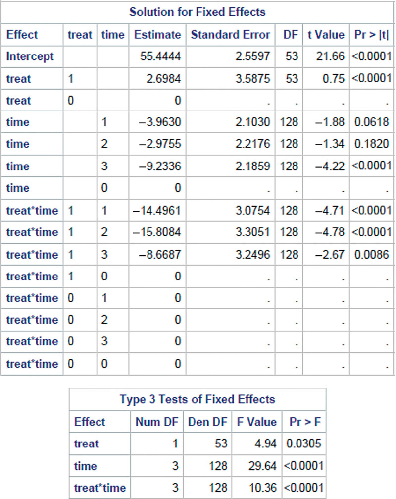
SAS Program output 5.2b presents the fixed-effect estimates of TREAT, TIME, and their interaction in the linear model on the PCL score. Given the statistical significance of the interaction term, the main effects of TREAT and TIME are both regarded as statistically meaningful. Therefore, all the fixed-effect estimates are statistically significant. (In reality, acupuncture treatment cannot have an actual effect on the PCL score at baseline; the issue about the main effect of treatment will be discussed in Chapter 7.) The Type 3 tests of the fixed effects provide further evidence that the overall fixed effects of treatment, time, and their interactions are all statistically significant (TREAT: F = 4.94, p = 0.0305; TIME: F = 29.64, p < 0.0001; TREAT by TIME: F = 10.36, p < 0.0001). The intercept, 55.44, is the population estimate of the mean PCL score at baseline for those in the control group, as the control group and the baseline time are each used as the reference level in specifying the two classification factors.
Given the specified interaction between time and treatment, it is difficult to generate the pattern of change over time in the PCL score from the fixed effects, let alone the difference between the two treatment groups. This lack of interpretability in the fixed effects is the reason why the least squares means are often computed to display the trajectory of individuals in the response variable. The following two output tables display the results of the least squares means and of the local tests.
SAS Program Output 5.2c:


The least square means, presented in the first panel and all statistically significant, display a much sharper decline in the PCL score among those receiving acupuncture treatment than among those in the control group. The mean PCL score of the treated patients drops from 58.14 at baseline to 39.68 at 1-month follow-up, and this dropped PCL then remains almost unchanged at 2-month follow-up (39.36) and at 3-month follow-up (40.24). In contrast, among those in the control group, the PCL score only declines slightly, from 55.44 at baseline to 51.48 at 1-month follow-up, 52.47 at 2-month follow-up, and 46.21 at 3-month follow-up. The results of the local tests on the group differences in the PCL score are presented in the second table. At baseline, the PCL difference between the two treatment groups, 2.70, is not statistically significant (t = −0.75, p = 0.4533), as can be anticipated from a randomized controlled trial design (the acupunctural treatment is not implemented until after the baseline time). The differences at the second and third time points, −11.80 and −13.11, respectively, are statistically significant (at the second time: t = −3.19, p = 0.0018; at the third time: t = −3.37, p = 0.0010), thereby suggesting that the acupuncture treatment significantly reduces PTSD symptom severity. At the last time point, the difference in the PCL score between the two treatment groups is not statistically significant (t = −1.55, p = 0.1224).
Lastly, the predicted PCL scores are plotted to display the time trends in the PCL score for the two treatment groups. Figure 5.1 displays two PCL trajectory curves for those who receive acupuncture treatment and those in the control group, respectively.

Figure 5.1 Time Trends of Predicted PCL Score: Acupunctural Treatment Versus Control
The plots in Fig. 5.1 display the strong impact acupuncture treatment has on reduction in PTSD symptom severity. During the first month after treatment, a patient who has received acupuncture treatment is expected to experience a much sharper decline in the PCL score than his or her counterpart in the control group, which is statistically meaningful. After the first month, this reduced severity score stabilizes throughout the rest of the observation period. The above model-based time plots of trends are strikingly similar to those in Fig. 4.2, suggesting that the two approaches handling intraindividual correlation, by specifying the between-subjects random effects and including a residual covariance matrix, generate very close results on the time trend and its group difference.
5.6.2. Linear regression model on marital status and disability severity among older Americans
In the second example, I perform the same type of analysis specified in Chapter 4 but using a different perspective to handle intraindividual correlation. The same AHEAD data of six waves are used (1998, 2000, 2002, 2004, 2006, and 2008), with the research objective remaining on the effect of marital status on the ADL count and its changing pattern over time. The dependent variable, ADL_COUNT, includes five activities of daily living: dress, bath/shower, eat, walk across time, and get in/out of bed. Other than the time factor, the covariates include the time-varying covariate married (1 = currently married and 0 = else) and three centered control variables (Age_mean, Educ_mean, and Female_mean). With the use of a residual variance–covariance matrix to account for intraindividual correlation, time is specified as a classification factor with six discrete levels (T = 0, 1, 2, 3, 4, and 5).
As indicated earlier, the first step in performing this type of analysis is to select an appropriate residual variance–covariance structure. As time intervals in the AHEAD survey, starting from 1998, are roughly equally spaced, I continue to use CS, AR(1), and TOEP as the three candidates for the selection of an appropriate covariance structure. Below is the SAS program for the three linear models, including three covariance patterns.
SAS Program 5.3:
. . . . . .

In SAS Program 5.3, there are a number of distinctive modifications as compared to SAS Program 4.3a. First, the time factor is specified as a classification factor, included in the CLASS statement with using TIME = 0 as the reference level. Second, the REPEATED statement replaces the RANDOM statement to specify three residual variance–covariance structures, CS, AR(1), and TOEP, respectively. The SUBJECT = HHIDPN option specifies the blocks of the R matrix. The options R and RCORR are interpreted previously. The three sets of model fit statistics are presented below.
SAS Program Output 5.3:
Fit Statistics with CS

Fit Statistics with AR(1)

Fit Statistics with TOEP

It can be concluded from SAS Program Output 5.3 that the TOEP covariance pattern model fits the AHEAD longitudinal data best, as each of its fit statistics has the smallest value among the three regression models. Given the selection of the TOEP covariance pattern model, the least squares means of the ADL count are computed at each time point and for those currently married and those currently not married, respectively. In the least square predictions, values of the three control variables are held constant at sample means to adjust for potential confounding effects. Significance tests of the ADL contrasts between the two marital status groups are performed by the ESTIMATE statement in the PROC MIXED procedure. Lastly, the predicted ADL counts at the six time points are plotted to display the time trend in the ADL count among older Americans and its difference between those currently married and those currently not married. The following is the SAS program for these analytic steps.
SAS Program 5.4:
. . . . . .

SAS Program 5.4 follows the same steps as those of SAS Program 5.2, except for a different set of variables, the extension of time points, and the use of a different residual variance–covariance structure. The PLOTS = ALL option, added to the PROC MIXED statement, tells SAS to produce all the plots appropriate for the analysis given a large sample size of the AHEAD longitudinal data. First, the TOEP covariance parameter estimates are displayed.
SAS Program Output 5.4a:

As indicated in Section 5.1, there are n residual variance–covariance parameters in the TOEP variance–covariance structure. Therefore, there are altogether six covariance parameters, including the variance of residuals. The five covariance parameters are estimated as 1.27 for TOEP(2), 0.93 for TOEP(3), 0.85 for TOEP(4), 1.01 for TOEP(5), and 1.52 for TOEP(6), all statistically significant (p < 0.0001). The variance estimate of residuals, assumed to be constant throughout the entire period of time, is 2.01, also statistically significant (p < 0.0001). As the selected covariance structure in this analysis, the TOEP residual variance–covariance pattern model is shown to explain a considerable portion of the total variance in residuals.
Next, the analytic results of the regression model, including solutions for the fixed effects and the Type 3 tests, are reported in Output 5.4b.
SAS Program Output 5.4b:


SAS Program Output 5.4b displays the estimates of the fixed effects and the Type 3 test results given the inclusion of the TOEP covariance matrix. The fixed-effect estimates are consistent with those presented in Table 4.3. Given the currently not married being used as the reference, the fixed effect of marital status, time-varying, is negatively associated with the ADL count, and therefore, those currently married are expected to have a lower ADL count than those currently not married, other covariates being equal. This fixed main effect of marital status, however, is not statistically significant ( ). All the regression coefficients of the discrete time factor are statistically significant (p < 0.0001) and so are those of the interaction terms, except for the interaction at the fifth time point (TIME = 4). The fixed main effects of time, combined, display an increasing trend over time in the ADL count among those currently not married. The regression coefficients of the three control variables are identical or very close to those reported in Table 4.2 (βage = 0.07, p < 0.0001; βedu = −0.06, p < 0.0001; βfemale = 0.30, p < 0.0001). Finally, the Type 3 tests of the fixed effects summarize the overall statistical significance of the fixed effects, suggesting that all the fixed effects, including that of the interaction term, are statistically significant.
The next output table displays the least squares means, classified by the two marital status groups and at the six time points.
SAS Program Output 5.4c:


The table for the least squares means presents that for both the currently married and the currently not married, the ADL count increases steadily over time, after adjusting for the confounding effects of the three control variables. At each time point, those currently married are expected to have a considerably lower ADL count than those currently not married, thereby suggesting a strong effect of current marriage on reduction in disability severity among older Americans. Results of the statistical significance tests on the ADL contrasts are presented next.
SAS Program Output 5.4d:

The results of the local tests suggest that the ADL contrasts between those currently married and those currently not married are statistically significant at all the time points except the baseline and the fifth points (Time = 0 and Time = 4). Unlike the case in randomized controlled clinical trials, the contrast at baseline is theoretically meaningful in the analysis of longitudinal data from observational surveys (Fitzmaurice et al., 2004) although in this analysis the baseline contrast is not statistically significant (this issue will be further discussed in Chapter 7).
Figure 5.2 graphically demonstrates longitudinal trajectories of the ADL count and the differences between those currently married and those currently not married.

Figure 5.2 Time Trends of Predicted ADL Score for Currently Married Versus Not Married
In Fig. 5.2, the blue and the red curves display the time trends for those currently married and those currently not married, respectively, with the straight lines from linear predictions taking time as a continuous variable. The two yellow curves describe the time trend in the entire population, assuming a balanced design. For both marital status groups, the ADL count increases over time, consistent with the pattern generally observed. Furthermore, the graph displays distinct separations between the curves associated with the two marital status groups, after adjusting for the confounding effects of age, education, and gender.
Least squares means can also be computed in the random intercept or the random coefficient model. Specifically, the least squares means can be computed given specified values of exact times. For example, such predictions can be calculated at the six time points for the two marital status groups by adding the specification of least squares means to SAS Program 4.3, as shown in the following SAS Program.
SAS Program 5.5:
. . . . . .

SAS Program 5.5 specifies a linear random coefficient model. In a series of LSMEANS statements, SAS is informed to compute the least squares means at six exact times by each marital status group. As in the random coefficient model time is a continuous variable. The ADL count can be predicted at as many time points as desired (e.g., at times 0, 0.1, 0.2, …, 4.9, 5.0), thereby yielding an approximately continuous time trend curve. As only the linear component of the time factor is considered in this linear random coefficient model, the least squares means of the ADL count are linearly associated with time, as displayed in Fig. 5.3.

Figure 5.3 Time Trends of Predicted ADL Score for Currently Married Versus Not Married: Random Coefficient Model
Figure 5.3 displays that for those currently married or those currently not married, the predicted ADL count is linearly associated with time. With the specification of the interaction term between time and marital status, the two straight lines have different slopes, other covariates being equal.
5.7. Summary
This chapter introduces a unique perspective in modeling normal longitudinal data, in which intraindividual correlation is accounted for by including a selected residual variance–covariance matrix, rather than by specifying the random effects. In this approach, the time factor must be specified as a classification factor with a series of discrete levels. A number of popular variance–covariance pattern models are described, with the strengths and limitations of each being discussed. These covariance pattern models can be divided into two categories: the covariance structures with time intervals equally spaced and the covariance pattern models with unequally spaced time intervals. Based on the description of various variance–covariance pattern models, I delineate the standard and the statistical methods to select an appropriate variance–covariance structure in residuals. In this chapter, the construction of the scaling matrices is also described for both the time factor and its interaction with another classification factor. It is sometimes difficult to generate a pattern of change over time directly from a combination of the time’s effects and its interactions with other classification factors. Therefore, I delineate the approach of least squares means extensively that are used as linear predictions of longitudinal trajectories for a hypothetically balanced population.
There are a number of distinctive advantages to using this modeling perspective in longitudinal data analysis. Essentially, this approach is a natural extension of repeated measures analysis of variance that specifies covariates as categorical and the dependent variable as continuous, and therefore, it is straightforward to interpret the analytic results. Given the tremendous simplicity and convenience by simply including a residual covariance pattern matrix, the researcher does not have to specify the subject-specific random effects, often with complex structures. The major disadvantage of using this perspective is that the analytic results do not often directly yield a pattern of change over time in the response variable as time is specified as a qualitative factor. In different situations, the linear mixed model specifying the random effects and the linear regression, including a residual covariance structure, are associated with their respective strengths and limitations. In biomedical research, a researcher’s interest is primarily in the effectiveness of a medical treatment or medication on disease, and therefore, the shape of the longitudinal trajectory of the outcome is not of direct concern. In such cases, the approach described in this chapter is popular and has been widely applied given its simplicity and convenience. Social researchers and demographers are generally more interested in the long-term time trend of a social, behavioral, or a health-related phenomenon. Large-scale survey data are generally used and time intervals are wide. In those situations, linear mixed models, in which time is a continuous variable, may be more useful in generating a long-term time trend, thereby providing important policy implications.
..................Content has been hidden....................
You can't read the all page of ebook, please click here login for view all page.