11.1. Overview of multinomial logistic regression model

$\text{Log}\left(\frac{P_{ik}}{P_{i\left(K+1\right)}}\right)={X^{\prime }}_i{\beta }_k,k=\mathrm{1,...},K\text{,}$

(11.1)

$P_{ik}=\mathrm{Pr}(Y_i=k\left|X_i\right.)={\left[1+\sum _{l=1}^K\exp ({X^{\prime }}_i{\beta }_l)\right]}^{-1}\exp ({X^{\prime }}_i{\beta }_k)\text{.}$

(11.2)

$P_{i\left(K+1\right)}=\mathrm{Pr}(Y_i=K+1\left|X_i\right.)={\left[1+\sum _{l=1}^K\exp ({X^{\prime }}_i{\beta }_l)\right]}^{-1}\text{.}$

(11.3)

$L=\prod _{i=1}^N{(P_{i1})}^{Y_{i1}}{P_{i2}}^{Y_{i2}}\mathrm{...}{\left[P_{i(K+1)}\right]}^{Y_{i(K+1)}}\text{,}$

(11.4)

$l=\sum _{i=1}^N\sum _{k=1}^{K+1}{Y}_{ik}\hspace{0.17em}\log (P_{ik}).$

(11.5)

Maximizing Equation (11.5) requires that this log-likelihood function be differentiated with respect to β using the standard procedures described in Chapter 8. In the construct of the multinomial logit regression model, the score statistic, mathematically defined as the first partial derivative of the log-likelihood function with respect to β and denoted by $\tilde{U}(\beta )$, is

$\begin{array}{c}\tilde{U}(\beta )=\frac{\partial l}{\partial \beta }=\sum _{i=1}^N\sum _{k=1}^{K+1}\frac{Y_{ik}}{P_{ik}}\frac{\partial P_{ik}}{\partial \beta }\\ =\sum _{i=1}^N\sum _{k=1}^{K+1}{Y}_{ik}\left[X_{ik}-\text{E}(X_i)\right],\end{array}$

(11.6)

$\text{E}(X_i)={\left[1+\sum _{l=1}^K\exp ({X^{\prime }}_i{\beta }_l)\right]}^{-1}\left[1+\sum _{l=1}^K\exp ({X^{\prime }}_i{\beta }_l)\right]X_i\text{.}$

$\begin{array}{c}\frac{{\partial }^{2}l}{\partial \beta \partial {\beta }^{\prime }}=\sum _{i=1}^N\sum _{k=1}^{K+1}\frac{Y_{ik}}{P_{ik}}\left[\frac{{\partial }^2{P}_{ik}}{\partial \beta \partial {\beta }^{\prime }}-\frac{1}{P_{ik}}\frac{\partial P_{ik}}{\partial \beta }\frac{\partial P_{ik}}{\partial {\beta }^{\prime }}\right]\\ =-\sum _{i=1}^N\sum _{k=1}^{K+1}{P}_{ik}\left[X_{ik}-\text{E}(X_i)\right]\hspace{0.17em}{\left[X_{ik}-\text{E}(X_i)\right]}^{\prime }.\end{array}$

(11.7)

As defined, the negative of the expectation of the second derivatives with respect to β of the log-likelihood function is the Fisher information, denoted by I(β). Given the expectation of the score to be zero, the Fisher information matrix yields the estimated variances and covariances of $\tilde{U}(\beta )$.

$\tilde{U}(\beta )=\frac{\partial l}{\partial \beta }=0\text{.}$

(11.8)

The previous procedure is the formalization of the maximum likelihood estimator in GLM given the link function specified as the multinomial logit. For a large sample, $\widehat{\beta }$ is the unique solution of $\tilde{U}(\beta )=0$, and therefore, $\widehat{\beta }$ is consistent for β and distributed as multivariate normal, denoted by

$\widehat{\beta }\sim \text{N}\left[0\text{,}\widehat{I}{\left(\beta \right)}^{-1}\right]\text{,}$

(11.9)

where $\widehat{I}(\beta )$ is the observed Fisher information matrix

$I(\widehat{\beta })=-\left(\frac{{\partial }^{2}l(\widehat{\beta })}{\partial \widehat{\beta }\partial {\widehat{\beta }}^{\prime }}\right)\text{.}$

The previous equations do not specify a random component as the residual term is simply integrated out in the estimation of a general multinomial logit model. Such a modeling approach is based on the so-called independence from irrelevant alternatives (IIA) hypothesis (Amemiya, 1985; McFadden, 1974). This fixed-effects specification can usher in some specification problems given the multivariate nature of a multinomial response. In view of the constraint that a set of choice probabilities always sum up to unity, an increase in one probability implies corresponding variations in one or more of the others, thereby implying dependence in a set of log odds. The invalid hypothesis of independence in random errors does not necessarily result in biased regression coefficients given the statistical property that the asymptotic process $\sqrt{n}(\widehat{\beta }-{\beta }_0)$, where ${\beta }_0$ is the true parameter vector, tends to converge in probability to a normal vector with mean 0 and the covariance matrix $I^{-1}(\widehat{\beta }\text{,}t)$ for large samples. When used to predict marginalized probabilities, however, this fixed-effects logit perspective on the multinomial data does not yield robust and consistent estimators, as will be shown in the succeeding texts.

11.2. Mixed-effects multinomial logit models and nonlinear predictions

$\begin{array}{c}{P}_{ijk}=\mathrm{Pr}(Y_{ij}=k\left|X_{ij}\right.)={\left[1+\sum _{l=1}^K\exp ({X^{\prime }}_{ij}{\beta }_l+b_{il})\right]}^{-1}\exp ({X^{\prime }}_{ij}{\beta }_k+b_{ik})\\ \\ ={\left[1+\sum _{l=1}^K\exp ({X^{\prime }}_{ij}{\beta }_l)\exp (b_{il})\right]}^{-1}\exp ({X^{\prime }}_{ij}{\beta }_k)\exp (b_{ik}),\end{array}$

(11.10)

where X_ij is the M × 1 covariate vector for subject i at time point j, including, in the context of longitudinal analysis, a time variable or a set of time polynomials. Likewise, β_k is the M × 1 vector of unknown regression parameters to be estimated, and b_ik is the between-subjects random effect on the kth logit component, assumed to be distributed as $\text{N}(\text{0,}{\sigma }_{b_k}^2)$. The probability P_ij(K+1) is the reference or residual probability, as indicated earlier.

$\begin{array}{c}{P}_{ijk}=\mathrm{Pr}(Y_{ij}=k\left|X_{ij}\right.)={\left[1+\sum _{l=1}^K\exp ({X^{\prime }}_{ij}{\beta }_l+b_{il}+{\varepsilon }_{ijl})\right]}^{-1}\exp ({X^{\prime }}_{ij}{\beta }_k+b_{ik}+{\varepsilon }_{ijk})\\ ={\left[1+\sum _{l=1}^K\exp ({X^{\prime }}_{ij}{\beta }_l)\exp (b_{il}+{\varepsilon }_{ijl})\right]}^{-1}\exp ({X^{\prime }}_{ij}{\beta }_k)\exp (b_{ik}+{\varepsilon }_{ijk}),\end{array}$

(11.11)

where ${\varepsilon }_{ijk}$ is the within-subject random disturbance distributed as $\text{N}(\text{0,}{\sigma }_{{\varepsilon }_{ijk}}^2)$.

$\log \left(\frac{P_{ijk}}{P_{ij\left(K+1\right)}}\right)={X^{\prime }}_{ij}{\beta }_k+b_{ik}+{\varepsilon }_{ijk}\text{,}\text{where}k=\text{1,}\mathrm{...}\text{,}K\text{.}$

(11.12)

Given the approximates of ${\sigma }_{{\varepsilon }_{ijk}}^2$, the probability that Y_ij = k (k = 1, …, K) for person i at time point j can be predicted by retransforming the linear predictor specified in Equation (11.12), given by

$\begin{array}{l}{\widehat{P}}_{ijk}={\left[1+\sum _{l=1}^K\text{exp}({X^{\prime }}_{ij}{\widehat{\beta }}_l){\widehat{\Phi }}_{ijl}\right]}^{-1}\text{exp}({X^{\prime }}_{ij}{\widehat{\beta }}_k){\widehat{\Phi }}_{ijk}\text{,}\\ \text{for}k=\text{1,}\mathrm{...}\text{,}K;l=\text{1,}\mathrm{...}\text{,}K,\end{array}$

(11.13)

where ${\widehat{\Phi }}_{ijk}=\exp (b_{ik}+{\varepsilon }_{ijk})$ is the estimated multiplicative random effect variable for subject i at time point j on response level k (k = 1, …, K). Given the definition of a lognormal distribution, the expectation of the posterior predictive distribution for the random variable is

$\text{E}({\Phi }_{ijk}\left|b_{ik}\right.)=\exp \left(\frac{{\sigma }_{b_{ik}}^2+{\sigma }_{{\varepsilon }_{ijk}}^2}{2}\right)\text{,}$

$\mathrm{var}({\Phi }_{ijk}\left|b_{ik}\right.)=\exp \left[2\left({\sigma }_{b_{ik}}^2+{\sigma }_{{\varepsilon }_{ijk}}^2\right)-\exp \left({\sigma }_{b_{ik}}^2+{\sigma }_{{\varepsilon }_{ijk}}^2\right)\right]\text{.}$

In the literature of statistics and econometrics, Equation (11.13) is defined as the inverse link function of the mixed-effects multinomial logit model, with the random components parameterized by two variance terms. The positive skewness of the lognormal distribution mandates that the expectation of Φ_ijk is greater than unity, with equality holding if and only if ${\sigma }_{b_{ik}}^2={\sigma }_{{\varepsilon }_{ijk}}^2=0$. Obviously, as is the case in the mixed-effects binary logit model, only using the fixed effects does not yield an unbiased prediction of a given probability marginalized at X_ij, even if the true value of β is known. Conditionally on β_k, the vectors of variances for the between-subjects effects and for the within-subject random errors with K levels, written as V_i(O) and V_ij(E), respectively, contain values ${\left\{{\sigma }_{b_{i1}}^2,\mathrm{...},{\sigma }_{b_{iK}}^2\right\}}^{\prime }$ and ${\left\{{\sigma }_{{\varepsilon }_{ij1}}^2,\mathrm{...},{\sigma }_{{\varepsilon }_{ijK}}^2\right\}}^{\prime }$, with the latter varying over different time points. The relative size of ${\left\{{\sigma }_{b_{i1}}^2,\mathrm{...},{\sigma }_{b_{iK}}^2\right\}}^{\prime }$ determines whether within-subjects random errors can be left unspecified in the prediction of K + 1 probabilities at a series of time points. As ${\sigma }_{{\varepsilon }_{ijk}}^2$ depends on the mean logit given the specification of the variance function, the variance of the joint random variable is not constant across time points, even with the specification of CS for the covariance structure of the between-subjects random effects.

$\begin{array}{c}{P}_{ijk}=\mathrm{Pr}(Y_{ij}=k\left|X_{ij}\right.)={\left[1+\sum _{l=1}^K\exp ({X^{\prime }}_{ij}{\beta }_l+{Z^{\prime }}_{ij}{b}_{il}+{\varepsilon }_{ijl})\right]}^{-1}\exp ({X^{\prime }}_{ij}{\beta }_k+{Z^{\prime }}_{ij}{b}_{ik}+{\varepsilon }_{ijk})\\ ={\left[1+\sum _{l=1}^K\exp ({X^{\prime }}_{ij}{\beta }_l)\exp ({Z^{\prime }}_{ij}{b}_{il}+{\varepsilon }_{ijl})\right]}^{-1}\exp ({X^{\prime }}_{ij}{\beta }_k)\exp ({Z^{\prime }}_{ij}{b}_{ik}+{\varepsilon }_{ijk}),\end{array}$

(11.14)

$\text{E}({\Phi }_{ijk}\left|b_{ik}\right.)=\exp \left(\frac{Z_{ij}{G}_k{Z^{\prime }}_{ij}+{\sigma }_{{\varepsilon }_{ijk}}^2}{2}\right)\text{,}$

(11.15)

$\mathrm{var}({\Phi }_{ijk}\left|b_{ik}\right.)=\exp \left[2(Z_{ij}{G}_k{Z^{\prime }}_{ij}+{\sigma }_{{\varepsilon }_{ijk}}^2)-\exp (Z_{ij}{G}_k{Z^{\prime }}_{ij}+{\sigma }_{{\varepsilon }_{ijk}}^2)\right]\text{.}$

(11.16)

If ${\widehat{\Phi }}_{ijk}$ and X_ij are replaced with $\text{E}\left({\Phi }_{ijk}\right)$ and X₀, respectively, Equation (11.13) predicts the marginal probability for a group of subjects with covariates valued at X₀, with individual probabilities within the group randomly scattered around the marginalized probability. The relationship between the subject-specific and the marginal probabilities has been well documented in the literature of nonlinear longitudinal data analysis (Diggle et al., 2002; Molenberghs and Verbeke, 2010) and is discussed in Chapter 10. Because the expected value of ${\widehat{\Phi }}_{ijk}$ is greater than unity, it is inappropriate to overlook this retransformed random variable in a prediction of a marginal probability unless ${\sigma }_{b_{ik}}^2={\sigma }_{{\varepsilon }_{ijk}}^2=0$ (Molenberghs and Verbeke, 2010). The specification of the marginal probability function based on the conditional perspective is useful for the derivation of interpretable results, nonlinear predictions, and demonstration of longitudinal trajectories of the response probabilities in the application of the mixed-effects multinomial logit model, as will be displayed later in the chapter.

11.3. Estimation of fixed and random effects

Let θ be the vector of parameters with elements β and $V\left(O\right)$. Then, for subject i, the likelihood function in the mixed-effects multinomial logit model can be written as a joint probability, given by

$L\left(Y_i\left|\theta \right.\right)=\prod _{j=1}^{n_i}\prod _{k=1}^{K+1}{\left(P_{ijk}\right)}^{Y_{ijk}}\text{,}$

(11.17)

where Y_ik is 1 if the ith observation falls in response level k at time point j and is 0 if otherwise, and Y_i is the n_i × 1 response vector for subject i containing elements Y_ik. For k = 1, …, K, P_ijk is defined by Equation (11.11) or Equation (11.14), depending on the specification of the between-subjects random effects, random intercept, or random coefficient. The estimation of P_k+1 relies on the estimates of other probabilities in the same set, given by ${\widehat{P}}_{K+1}=1-{\widehat{P}}_1-\mathrm{...}-{\widehat{P}}_K$.

$l(Y_i\left|\theta \right.)=\sum _{j=1}^{n_i}\sum _{k=1}^{K+1}{Y}_{ijk}\log (P_{ijk}).$

(11.18)

$\text{E}\left(P_{ijk}\left|\theta \right.\right)={\int \text{g}}^{-1}\left[{X^{\prime }}_{ij}{\beta }_k+\log \left({\Phi }_{ijk}\right)\right]\text{d}F\left({\Phi }_{ij}\right)\text{,}$

(11.19)

where the error distributional function F is the cumulative density function, and ${\Phi }_{ij}$ is a vector of multiplicative random variables containing elements ${\left\{{\Phi }_{ij1},\mathrm{...},{\Phi }_{ijK}\right\}}^{\prime }$. In this integration, the differential term is written as dF(Φ_ij) instead of dF(Φ_ijk) because the prediction of the probability P_ijk involves all logit components. The term V_i(e) is not particularly specified in θ because within-subject random errors are considered to be embedded in the fixed effects in the multinomial logit regression model, thereby being integrated out (Amemiya, 1985; Zeger et al., 1988). If both ${\sigma }_{b_{ik}}^2$ and ${\sigma }_{{\varepsilon }_{ijk}}^2$ are sizable, the predicted probability ${\widehat{P}}_{ijk}$ can deviate markedly from the estimator ${\text{g}}^{-1}({X^{\prime }}_{ij}{\widehat{\beta }}_k)$. Because F is not a cumulative normal function, ${\widehat{P}}_{ijk}$ is often not ${\text{g}}^{-1}({X^{\prime }}_{ij}{\widehat{\beta }}_k)$, thereby indicating the importance of retransforming the random components in the mixed-effects multinomial logit model. Whether $\text{E}(P_{ijk}\left|\theta \right.)>g^{-1}({X^{\prime }}_{ij}{\widehat{\beta }}_k)$ or $\text{E}(P_{ijk}\left|\theta \right.)<g^{-1}({X^{\prime }}_{ij}{\widehat{\beta }}_k)$ depends on the relative size of Φ_ijk in Φ_ij.

$\frac{\partial \hspace{0.17em}l}{\partial \theta }=\sum _{i=1}^N{\text{g}}^{-1}(Y_i)\left[\frac{\partial \hspace{0.17em}\text{g}(Y_i)}{\partial \theta }\right]=0\text{.}$

(11.20)

$I\left(\theta \right)=\text{E}\left(-\frac{{\partial }^{2}l}{\partial \theta \partial {\theta }^{\prime }}\right)=\sum _{i=1}^N{\text{g}}^{-2}(Y_i)\frac{\partial \text{g}\left(Y_i\right)}{\partial \theta }{\left[\frac{\partial \text{g}(Y)}{\partial \theta }\right]}^{\prime }\text{.}$

(11.21)

11.4. Approximation of variance–covariance matrix on probabilities

Let $\widehat{\mathcal{L}}$ be a random vector of the predicted logit components ${(\widehat{\mathcal{L}}={\widehat{\mathcal{L}}}_1,{\widehat{\mathcal{L}}}_2,\mathrm{...},{\widehat{\mathcal{L}}}_K)}^{\prime }$ from Equation (11.12) with mean η and variance–covariance matrix $V(\widehat{\mathcal{L}})$, and $\widehat{P}={\text{g}}^{-1}(\widehat{\mathcal{L}})$ is a transform of $\widehat{\mathcal{L}}$, as defined by Equation (11.13), where g is the logit link function and g⁻¹ is its inverse function. For large samples, the first-order Taylor series expansion of ${\text{g}}^{-1}(\widehat{\mathcal{L}})$ yields approximation of mean

$\text{E}\left[{\text{g}}^{-1}(\widehat{\mathcal{L}})\right]\approx {\text{g}}^{-1}(\eta )\text{,}$

(11.22)

and the variance–covariance matrix $\widehat{V}(\widehat{P})$

$V\left[g^{-1}(\widehat{\mathcal{L}})\right]\approx {\left[\frac{\partial g^{-1}(\widehat{\mathcal{L}})}{\partial \widehat{\mathcal{L}}}\left|\widehat{\mathcal{L}}=\eta \right.\right]}^{\prime }\Sigma (\widehat{\mathcal{L}})\left[\frac{\partial g^{-1}(\widehat{\mathcal{L}})}{\partial \widehat{\mathcal{L}}}\left|\widehat{\mathcal{L}}=\eta \right.\right]\text{,}$

(11.23)

$\frac{\partial g^{-1}(\widehat{\mathcal{L}})}{\partial \widehat{\mathcal{L}}}=\left[\frac{\partial g_1^{-1}(\widehat{\mathcal{L}})}{\partial \widehat{\mathcal{L}}},\frac{\partial g_2^{-1}(\widehat{\mathcal{L}})}{\partial \widehat{\mathcal{L}}},\mathrm{...}\right]\text{,}$

$\Sigma (\widehat{\mathcal{L}})=\left(\begin{array}{l}\mathrm{var}({\widehat{\mathcal{L}}}_1)\text{cov}({\widehat{\mathcal{L}}}_1\text{,}{\widehat{\mathcal{L}}}_2)\cdot \cdot \cdot \mathrm{cov}({\widehat{\mathcal{L}}}_1\text{,}{\widehat{\mathcal{L}}}_K)\\ \\ \mathrm{var}({\widehat{\mathcal{L}}}_2)\cdot \cdot \cdot \mathrm{cov}({\widehat{\mathcal{L}}}_2\text{,}{\widehat{\mathcal{L}}}_K)\\ \\ \ddots \\ \mathrm{var}({\widehat{\mathcal{L}}}_K)\end{array}\right)\text{.}$

In Equation (11.23), the matrix $V\left[{\text{g}}^{-1}(\widehat{\mathcal{L}})\right]$ is the approximate of the variance–covariance matrix V(P) for large samples. The square roots of the diagonal elements in this variance–covariance matrix yield the standard errors of the predicted probabilities contained in the vector $\widehat{P}$ given $\widehat{\beta }$ and $\widehat{V}(\widehat{O})$. As a result, the confidence interval for the predicted probability ${\widehat{P}}_{ijk}$ can be easily computed.

The delta method depends on the validity of the Taylor series approximation, and therefore, some caution must be exercised before its adequacy is verified with simulation. In the context of the multinomial logit model, the application of the Taylor series expansion is well justified to approximate P and V(P) because ${\text{g}}^{-1}(\widehat{\mathcal{L}})$ is a smooth nonlinear function of $\widehat{\mathcal{L}}$. Consequently, the previous procedure usually provides a robust, one-on-one standard error estimator (Stuart and Ord, 1994). As indicated in Chapter 8, bootstrapping is sometimes applied to estimate the standard errors of nonlinear predictions. The bootstrap procedure, however, generates less efficient, robust approximates than a retransformation approach with known elements in $\Sigma (\widehat{\mathcal{L}})$ for the mixed-effects multinomial logit model because it is based on the assumption that the off-diagonal elements in $V(\widehat{\mathcal{L}})$ are all zero (Follmann, 1994). If the elements in $V(\widehat{\mathcal{L}})$ are unobtainable empirically, some covariance structure in the multinomial distribution needs to be assumed for the application of the bootstrap.

Because a subject’s probability is not empirically observable at a specific time point, the multinomial logit function does not have observed values on the logit components. Consequently, the variance–covariance matrix for the predicted logit is not empirically obtainable. Nevertheless, an approximation approach can be used to obtain an estimate of the matrix with K logit components by extending the perspective described in Chapter 10. First, fit a mixed-effects multinomial logit model with all covariates rescaled to be centered at some selected values. Second, use the squared standard error of each intercept estimate plus the corresponding variance of the between-subjects random effect as the variance for each of the K logit components. Third, take the off-diagonal elements in $\widehat{V}(\widehat{\mathcal{L}})$ as the estimate of covariance between each pair of the logit intercept estimates. The rationale for this approximation is that if covariates are rescaled to be centered at specified values, the intercepts represent the group-specific means of the logit components, and therefore, the local variance–covariance matrix for the estimated intercepts plus the corresponding between-subjects random effects can be considered the approximates of the variance–covariance matrix for the mean logit function. While it is computationally tedious, in Section 11.6 a detailed procedure of this approximation method will be described empirically.

11.5. Conditional effects of covariates on probability scale

As applied for the mixed-effects binary logit model, the discrete probability change approach (Long, 1997) can be applied to compute the conditional effect of a given covariate on the probabilities of a multinomial response. For illustrative convenience, in the following presentation, the subscripts ij in the notation of probability P_ijk are again temporarily removed from the mathematical expressions. That is, P_ijk is replaced with $P_k\left|X_0\right.$, indicating the probability of falling in the kth response level for a typical subject with covariate vector X₀ that includes the value of time at time point j.

Consider the continuous covariate first. Let X₀ be the vector containing the selected values of a set of covariates, including a time factor, and X_0r represents the vector containing the selected values of the covariates except for a specific continuous variable X_m. It follows that $({\widehat{P}}_k\left|X_0\right.)$ represents the marginalized estimate of $({\widehat{P}}_k\left|X\right.)$ when all the covariates are scaled at some purposefully selected values, with the value of X_m scaled as its sample mean. Likewise, let $({\widehat{P}}_k\left|{\overline{X}}_m+1\text{,}{X}_{0r}\right.)$ be another marginalized estimate of $({\widehat{P}}_k\left|X\right.)$ when X_m is scaled at one unit greater than its sample mean and other covariates are fixed at previously selected values. Then, the difference between $({\widehat{P}}_k\left|{\overline{X}}_m+1\text{,}{X}_{0r}\right.)$ and $({\widehat{P}}_k\left|X_0\right.)$ is defined as the conditional effect of covariate X_m on the probability of the response level k marginalized at the selected values of the covariates. Such a conditional effect is denoted by $∆{\widehat{P}}_{km}$, given by

$∆{\widehat{P}}_{km}=\frac{\text{exp}\left[{\widehat{\beta }}_{km}({\overline{X}}_m+1)+{X^{\prime }}_{0r}\hspace{0.17em}{\widehat{\beta }}_{kr}\right]{\widehat{\Phi }}_k}{1+\sum _{l=1}^K\text{exp}\left[{\widehat{\beta }}_{lm}({\overline{X}}_m+1)+{X^{\prime }}_{0r}\hspace{0.17em}{\widehat{\beta }}_{lr}\right]{\widehat{\Phi }}_l}-\frac{\text{exp}({X^{\prime }}_0\hspace{0.17em}{\widehat{\beta }}_k){\widehat{\Phi }}_k}{1+\sum _{l=1}^K\text{exp}({X^{\prime }}_0\hspace{0.17em}{\widehat{\beta }}_l){\widehat{\Phi }}_l}\text{,}$

(11.24)

where ${\widehat{\beta }}_{km}$ is the regression coefficient of X_m on the kth response level, and ${\widehat{\beta }}_{kr}$ is the (M − 1) × 1 vector of the unknown regression parameters for the covariates contained in X_0r.

If the index variable X_m is a dichotomous variable, the 0–1 change in that covariate should be specified. Accordingly, the conditional effect of X_m on the probability of the response level k is written as (11.25)

Given the mathematical constraints that a set of the probabilities for (K + 1) response categories always sum up to unity and the corresponding set of a covariate’s conditional effects must sum up to zero, the conditional effect of a covariate on the probability of the (K + 1)th level is defined as $∆{\widehat{P}}_{K+1,x_m}=-(∆{\widehat{P}}_{1x_j}+\mathrm{....}+∆{\widehat{P}}_{K{x}_j})$. In view of the restrictive conditions on the multinomial response, all the conditional effects of a given covariate on a set of probabilities should be considered statistically significant if any one of them is statistically significant, other covariates being equal (Liu and Engel, 2012). In other words, if the conditional effect of the covariate on one of the K log odds is statistically significant, the face values for the entire set of the conditional effects should be accepted.

Specifically, statistical significance of the conditional effect on the probability scale can be tested by using the Wald chi-square statistic, denoted by ${\chi }_{\text{W,}k}^2$ (Klein and Moeschberger, 2003; Liu, 2012), as also indicated in Chapter 10. In the context of mixed-effects multinomial logit models, let ${\widehat{P}}_{k0}$ represent $({\widehat{P}}_k\left|X_0\right.)$ and ${\widehat{P}}_{k1}$ stand for $({\widehat{P}}_k\left|{\overline{X}}_m+1\text{,}{X}_{0r}\right.)$. The following equation is then defined from the delta method:

${\chi }_{\text{W,}k}^2\approx \frac{{({\widehat{P}}_{k1}-{\widehat{P}}_{k0})}^2}{\widehat{V}({\widehat{P}}_{k0})+\widehat{V}({\widehat{P}}_{k1})-2\mathrm{cov}({\widehat{P}}_{k0}{\widehat{P}}_{k1})},k=1\text{,}\mathrm{...}\text{,}K\text{,}$

(11.26)

As extended from the binary to the multinomial response, Equation (11.26) bears a tremendous resemblance to Equation (10.29). Also analogous to the binary perspective, Equation (11.26) can be simplified as the two predicted probabilities, ${\widehat{P}}_{k0}$ and ${\widehat{P}}_{k1}$, are computed from the same parameter estimates and where all but one covariate have exactly the same values. Therefore, the two random variables P_k0 and P_K1 should follow the same probability distribution. Consequently, Equation (11.26) can reduce to

${\chi }_{\text{W},k}^2\approx \frac{{({\widehat{P}}_{k1}-{\widehat{P}}_{k0})}^2}{\widehat{V}({\widehat{P}}_{k0})+\widehat{V}({\widehat{P}}_{k1})-2\sqrt{\widehat{V}({\widehat{P}}_{k0})\widehat{V}({\widehat{P}}_{k1})}}\text{.}$

(11.27)

This Wald statistic is distributed asymptotically as chi-square with one degree of freedom under the null hypothesis that $({\widehat{P}}_{k1}-{\widehat{P}}_{k0})=0$. The evaluation of $∆{\widehat{P}}_{K+1}$, the residual effect in the same probability set, depends on the test results of the nonreference conditional effects. That is, if any nonreference conditional effect is significant, $∆{\widehat{P}}_{K+1}$ should be considered statistically significant; if all of the nonreference conditional effects are statistically insignificant, $∆{\widehat{P}}_{K+1}$ is not statistically significant.

11.6. Empirical illustration: marital status and longitudinal trajectories of disability and mortality among older Americans

11.6.2. Analytic steps with SAS programs

As the application of the PROC NLMIXED procedure in the SAS system requires the robust starting values of specified parameters, the PROC GLIMMIX procedure is used first to produce an initial set of parameter estimates, which are then borrowed as the robust starting values of both the fixed and the random effects to apply the PROC NLMIXED procedure. The following SAS program specifies this GLIMMIX model.

SAS Program 11.1:

In SAS Program 11.1, the outcome variable HEALTH_ST is created first given the aforementioned specification (1 = functionally disabled, 2 = dead between two successive waves, and 3 = functionally independent). Next, a multinomial logit model is constructed with the specification of a random intercept term. The options NOITPRINT and NOCLPRINT tell SAS not to print the “Iteration History” and “Class Level Information” tables. The METHOD = QUAD(QPOINTS = 1) option specifies the use of the adaptive Gaussian quadrature with a single quadrature point in each dimension of the integral within a GLMM framework. The CLASS statement specifies the classification variables used in this model, consisting of the dependent variable HEALTH_ST and a subject’s identification number HHIDPN. The predesigned residual variance–covariance structures, such as AR(1) and SP(POW), are not specified for a multinomial distribution in the PROC GLIMMIX procedure. As the probabilities for a multinomial response are not observable, variability in the response cannot be captured effectively to generate a robust variance–covariance structure. Consequently, for the mixed-effects multinomial logit model, the correlation between repeated measurements of the multinomial response for the same subject is modeled by means of the specified random effects.

In the MODEL statement, the dependent variable and the fixed effects are specified. Six covariates, described earlier, are considered in the model. The option S (or SOLUTION) requests the solution for the fixed-effects parameters. The DIST = MULTINOMIAL option specifies the distribution of the dependent variable to be multinomial. Correspondingly, the option LINK = GLOGIT specifies the link function in this specific GLMM to be generalized logit. Additionally, the COVB option asks SAS to produce the approximate variance–covariance matrix of the fixed-effects estimates, and DDFM = BW specifies the residual degrees of freedom to be divided into between-subjects and within-subjects components.

The RANDOM statement defines the Z matrix of the mixed model, as mentioned previously. In this illustration, Z contains only one element for each logit component, and correspondingly, the G matrix only includes the logit intercepts. The option SUBJECT = HHIDPN identifies the subjects in this random intercept multinomial logit model. Similarly, the GROUP = HEALTH_ST option identifies three groups by which to vary the covariance parameters.

Next, given the parameter estimates from the PROC GLIMMIX procedure, not presented, the starting values of parameters can be specified in the PROC NLMIXED procedure. The following SAS program presents code for the full random intercept multinomial logit model with time centered at four (T = time – 4, the third time point), and all other covariates centered at sample means.

SAS Program 11.2:

In the PROC NLMIXED statement, the MTHOD = GAUSS option calls for the application of the adaptive Gaussian quadrature, COV asks SAS to print the approximate covariance matrix for the parameter estimates needed for computing the standard errors of nonlinear predictions on the multinomial response, and QPOINTS = 3 tells SAS that three quadrature points be used in each dimension of the random effects. The PARMS statement specifies the starting values of the parameter estimates on two logit components, log(P₁/P₃) and log(P₂/P₃), obtained from the PROC GLIMMIX procedure. With the specification of starting values for both the fixed and the random effects, the PROC NLMIXED procedure estimates the regression coefficients of the covariates on the two logit components. The error terms u0010 and u0015 indicate the random effects on the two logit components, each of which is assumed to be multivariate normal with zero expectation. The specifications of “le-6” and “−le15” are used to approximate a range of log(P) values between minus infinity to zero. If the PARMS statement is not given, the NLMIXED procedure assigns the default value of 1.0. As indicated in Chapter 10, if the starting values are too distant from the final estimates, numerical integration techniques will not perform well for a nonlinear regression model. Additionally, without the RANDOM statement to specify the random terms u0010 and u0015 in the linear predictors, the parameter estimates and the corresponding standard errors will be identical to those from the PROC LOGISTIC or the PROC CATMOD procedure with the specification of the multinomial response.

The reduced-form BLUP and the retransformation method are based on the same random intercept multinomial logit model, eliminating variable EDUC_MEAN from statistical inference and estimation. While the BLUP predicts the probabilities for each observation (Littell et al., 2006), the group mean of the BLUPs, the so-called empirical BLUP, can be estimated by creating a scoring dataset specifying the multinomial outcome variable as missing and the independent variables as zero, with the covariates being centered at selected values corresponding to a specific population group. In the scoring data, the random effects per individual should be present, and therefore, the mean of the BLUPs with y = missing and X’s = 0 derives the predicted health probabilities for a group or an average person taking selected values of the covariates.

Below is the SAS program for the reduced-form random intercept multinomial logit model with time centered at four and the other covariates rescaled to be centered at sample means. The part for creating the scoring dataset is presented first.

SAS Program 11.3a:

In SAS Program 11.3a, a scoring dataset is created, and it is then combined with the main data through the DATA step. As a result, in the temporary dataset TP4 each subject has seven data points, six actual and one hypothetical. As the variable “t” is centered at four, the “t = 0” statement actually specifies the time factor in the scoring dataset as TIME = 4 (the third data point). As can be recognized, SAS Program 11.3a is identical to SAS Program 10.3a except the specification of a different outcome variable, HEALTH_ST.

With the creation of the scoring dataset and its combination with the main data, the reduced-form random intercept multinomial logit model can be constructed, as displayed in the following SAS program.

SAS Program 11.3b:

In the PROC NLMIXED procedure, the syntax is analogous to SAS Program 11.2 except for the removal of covariate EDUC_MEAN and the addition of the PREDICT statements to compute the BLUPs for each subject in the scoring dataset. As there are three nonlinear predictions for P₁, P₂, and P₃, respectively, three PREDICT steps are specified to predict three probabilities by using the fixed parameter estimates and the empirical Bayes estimates of the between-subjects random effects. The predicting results are then placed in three output datasets with the OUT = options (OUT1, OUT2, OUT3), and as a result, the means and the standard errors of three empirical BLUP predictions (PRED1, PRED2, PRED3) can be computed by the application of the PROC MEANS procedure.

The reduced-form fixed-effects multinomial logit model can be created by modifying SAS Program 11.3, removing the RANDOM and the PREDICT statements. Without the specification of the random intercepts, the empirical BLUP per individual cannot be produced, and therefore, the call for the PROC MEANS procedure is redundant. Below is the SAS program for this model.

SAS Program 11.4:

The previous random intercept multinomial logit models are specified just for analytic convenience and illustrative simplicity. The presentations shown in the illustration do not depend on the validity of those ad hoc models; any other more flexible mixed-effects multinomial logit models would lead to the same results concerning the statistical efficiency and coverage of the retransformation method. If a random coefficient multinomial logit model is applied, the variance–covariance structure becomes a block covariance matrix, thereby further increasing statistical complexity and the computational burden on the multinomial response. In the course of preparing this illustration, a random coefficient multinomial logit model is also created and analyzed by extending the random intercept perspective described earlier. For the reader’s reference, the model specifications and the corresponding SAS program for this random coefficient multinomial logit model are presented in Appendix D.

11.6.3. Analytic results and nonlinear predictions

Table 11.1 displays the analytic results of the three multinomial logit models described earlier. As indicated, the regression coefficients of covariates on the logit components do not provide interpretable information on the multinomial response. Therefore, in reading Table 11.1, the reader’s focus should be placed on the statistical significance of the parameter estimates and the differences in the estimates from the three models.

Table 11.1

Results of Three Multinomial Logit Models on Health States in Older Americans (N = 2000)

Explanatory Variable and Effect Type	Log (P1/P3)		Log (P2/P3)
	Parameter Est.	Standard Error	Parameter Est.	Standard Error
	Full Mixed-Effects Multinomial Logit Model
Fixed effects
Intercept	−0.938***	0.033	−1.964***	0.069
Time (centered at four)	0.152***	0.009	0.355***	0.024
Married_mean	−0.455***	0.072	0.170	0.110
Time × Married_mean	0.028	0.019	−0.066**	0.027
Age_mean	0.041***	0.006	0.183***	0.012
Educ_mean	−0.078***	0.009	−0.092***	0.013
Female_mean	0.358***	0.073	−0.409***	0.103
Random effects
Intercept	0.165***	0.030	0.413**	0.184
	Reduced Mixed-Effects Multinomial Logit Model
Fixed effects
Intercept	−0.939***	0.033	−1.965***	0.069
Time (centered at four)	0.143***	0.009	0.349***	0.025
Married_mean	−0.456***	0.071	0.169	0.110
Time × Married_mean	0.030	0.019	−0.066**	0.027
Age_mean	0.057***	0.006	0.189***	0.012
Female_mean	0.357***	0.072	−0.409***	0.102
Random effects
Intercept	0.166***	0.029	0.413**	0.188
	Reduced Fixed-Effects Multinomial Logit Model
Fixed effects
Intercept	−0.970***	0.031	−1.961***	0.051
Time (centered at four)	0.132***	0.010	0.441***	0.014
Married_mean	−0.460***	0.071	0.170	0.104
Time × Married_mean	0.030	0.021	−0.070***	0.026
Age_mean	0.117***	0.006	0.226***	0.008
Female_mean	0.360***	0.072	−0.410***	0.088

*    0.05 < p < 0.10; **0.01 < p < 0.05; ***p < 0.01.

Of the fixed effects displayed in Table 11.1, the regression coefficients of marital status on the second logit and the interaction between time and marital status on the first logit are not significant individually. Even so, given the statistical criterion about the fixed effects on a set of logit components, all the regression coefficients are viewed as statistically significant with α = 0.05. Therefore, the three multinomial logit models have the same test results on the logit coefficients. The regression coefficients of time on both logit components are positive and statistically significant. Marital status is negatively linked to the first logit component but is positively associated with the second. The regression coefficient of the interaction between time and marital status is positive on the first and is negative on the second logit component, other covariates being equal. All the three control variables yield very strong effects on the multinomial logit components. Caution must apply, however, in attempting to interpret the fixed effects substantively.

In the two random intercept multinomial logit models, the full and the reduced, the between-subjects random effects on the two logit components are 0.17 and 0.41, respectively, both statistically significant. The strong random effects indicate the importance of specifying the random effects in modeling the multinomial longitudinal data.

The analytic results derived from the reduced-form random intercept multinomial logit model are very close, some even identical, to those from the full model, both the point and the standard error estimates. Additionally, the reduced fixed-effects multinomial logit model yields close estimates of the fixed effects to those from the two mixed-effects multinomial logit models. In the application of GLMM-type models, such a similarity is not surprising given the desirable property that the asymptotic process $\sqrt{n}(\widehat{\beta }-{\beta }_0)$, where ${\beta }_0$ is the true parameter vector, tends to converge in probability to a normal vector with mean 0 and the covariance matrix $I^{-1}(\widehat{\beta }\text{,}t)$ for large samples, even in the presence of strong clustering in Y (Davidian and Giltinan, 1995; Liang and Zeger, 1986; Zeger et al., 1988; Liu and Engel, 2012). It does not mean, however, that the fixed-effects multinomial logit model can yield robust and consistent estimators for nonlinear predictions of the probabilities in the longitudinal setting, as will be shown in the succeeding texts.

The probability of each health state at each time point and the corresponding variance can be estimated by applying Equations (11.22) and (11.23), respectively. In the context of this illustration, four partial derivatives of two predicted probabilities are identified with respect to two logit components. For ${\widehat{P}}_1$, we have

$\frac{\partial {\widehat{P}}_1}{\partial {\widehat{\mathcal{L}}}_1}={\left\{{\left[1+\sum _{k=1}^2\exp ({\widehat{\mathcal{L}}}_k)\right]}^2\right\}}^{-1}\exp ({\widehat{\mathcal{L}}}_1)\left[1+\exp ({\widehat{\mathcal{L}}}_2)\right]=B_{11}\text{,}$

(11.28a)

$\frac{\partial {\widehat{P}}_1}{\partial {\widehat{\mathcal{L}}}_2}={\left\{{\left[1+\sum _{k=1}^2\exp ({\widehat{\mathcal{L}}}_k)\right]}^2\right\}}^{-1}\left[-\exp ({\widehat{\mathcal{L}}}_1)\exp ({\widehat{\mathcal{L}}}_2)\right]=B_{12}\text{.}$

(11.28b)

Likewise, the corresponding partial derivatives for ${\widehat{P}}_2$ are

$\frac{\partial {\widehat{P}}_2}{\partial {\widehat{\mathcal{L}}}_1}={\left\{{\left[1+\sum _{k=1}^2\exp ({\widehat{\mathcal{L}}}_k)\right]}^2\right\}}^{-1}\left[-\exp (\widehat{\mathcal{L}})\exp ({\widehat{\mathcal{L}}}_2)\right]=B_{21}\text{,}$

(11.28c)

$\frac{\partial {\widehat{P}}_2}{\partial {\widehat{\mathcal{L}}}_2}={\left\{{\left[1+\sum _{k=1}^2\exp ({\widehat{\mathcal{L}}}_k)\right]}^2\right\}}^{-1}\exp ({\widehat{\mathcal{L}}}_2)\left[1+\exp ({\widehat{\mathcal{L}}}_1)\right]=B_{22}\text{.}$

(11.28d)

Let

$\left[\frac{\partial {\text{g}}^{-1}(\widehat{\mathcal{L}})}{\partial \widehat{\mathcal{L}}}{\left|\hspace{0.17em}\right.}_{\mathcal{L}=\mu }\right]=B\text{,}$

where

$B=\left(\begin{array}{l}{B}_{11}{B}_{12}\\ B_{21}{B}_{22}\end{array}\right)\text{.}$

The variance–covariance matrix for the predicted probabilities ${\widehat{P}}_1$ and ${\widehat{P}}_2$ in this analysis can then be approximated by the following sandwich estimator:

$V(\widehat{P})\approx \mathrm{B\Sigma }(\widehat{\mathcal{L}})B^{\prime }\text{,}$

(11.29)

where

$\Sigma (\widehat{\mathcal{L}})=\left(\begin{array}{l}{\sigma }_{•1}^2{\sigma }_{12}\\ {\sigma }_{21}{\sigma }_{•2}^2\end{array}\right)\text{.}$

In the retransformation method, the total variance is defined as ${\sigma }_{•k}^2=\hspace{0.17em}{\sigma }_{b_k}^2+{\sigma }_{e_k}^2$, where k = 1, 2, consisting of two random components: between-subjects and within-subject. In the empirical BLUP, on the other hand, only ${\sigma }_{b_k}^2$ is included in predicting the probabilities (Littell et al., 2006).

To highlight disparities in different predicting methods, four sets of the probabilities are predicted on the three health states at six time points, using analytic results from the full random intercept multinomial logit model, the retransformation method, the empirical BLUP, and the fixed-effects multinomial logit model, respectively. Table 11.2 presents the sets of the predicted probabilities and the corresponding standard errors at six time points.

Table 11.2

Predicted Probabilities of Disability and Death at Six Time Points

Health State	Time Point
	T0 (1998)	T1 (2000)	T2 (2002)	T3 (2004)	T4 (2006)	T5 (2008)
	Predicted Probability Generated From the Full Model
Disabled	0.256	0.259	0.266	0.268	0.271	0.260
	(0.066)	(0.068)	(0.082)	(0.084)	(0.087)	(0.072)
Dead	–	0.108	0.108	0.112	0.114	0.112
		(0.064)	(0.063)	(0.065)	(0.068)	(0.066)
	Predicted Probability Generated From the Retransformation Approach
Disabled	0.257	0.258	0.266	0.268	0.271	0.260
	(0.068)	(0.070)	(0.082)	(0.084)	(0.087)	(0.072)
Dead	–	0.108	0.108	0.112	0.114	0.112
		(0.063)	(0.063)	(0.065)	(0.068)	(0.066)
	Predicted Probability Generated From BLUP
Disabled	0.248	0.253	0.259	0.259	0.246	0.249
	(0.023)	(0.025)	(0.035)	(0.037)	(0.039)	(0.027)
Dead	–	0.089	0.095	0.102	0.108	0.109
		(0.020)	(0.020)	(0.022)	(0.023)	(0.020)
	Predicted Probability Generated From the Fixed-Effects Approach
Disabled	0.251	0.250	0.250	0.250	0.250	0.253
	(0.008)	(0.007)	(0.006)	(0.007)	(0.009)	(0.009)
Dead	–	0.093	0.093	0.093	0.093	0.094
		(0.005)	(0.004)	(0.004)	(0.006)	(0.010)

Note:    The predicted probability of “not disabled” and its standard error depend on the results for the probabilities of the other two health states, therefore they are not displayed in the table.

AHEAD Longitudinal Survey (N = 2000).

In Table 11.2, the probability of disability is shown to stabilize over time at the baseline level, reflecting the result of a selection of the fittest process among this very old population (in 1998, the youngest member of the AHEAD cohort was age 75 years). Therefore, after including mortality as a competing risk in the mixed-effects logit modeling, the increasing trend over time in the probability of disability shown in Chapter 10 vanishes. This stable pattern of change agrees with the time trend of health often observed in older populations. While individually disability tends to get intensified over age, collectively survivors are those who are more physically fit than those deceased, thereby altering the population health composition dynamically. This pattern of disparity between individual aging and population health is particularly observable in the oldest old. Here, selection of individuals offsets the effect of population aging. Therefore, in studies for older persons, it is imperative to account for the selection effect in the analysis of longitudinal qualitative data. In Table 11.2, the mortality rate is also shown to be constant throughout the entire observation period, perhaps due to the same selection effect.

Given the relatively small size of the standard errors for the probabilities of disability and mortality, all the predicted probabilities displayed in Table 11.2 are considered statistically significant. The retransformation method, after one theoretically important, statistically significant predictor is removed, yields very close predictions, both the point estimates and the standard error approximates, to those from the full random intercept multinomial logit model. Therefore, in the construct of the mixed-effects multinomial logit model, the retransformation method is shown to have statistically adequate capacity for handling unobserved heterogeneity in nonlinear predictions. The empirical BLUP provides fairly close predictions at the early time points; in the last three time points, however, the predicted probabilities deviate markedly from those of the first two approaches. Furthermore, the empirical BLUP, not accounting for inherent within-subject variability, results in the severely underestimated standard errors of the nonlinear predictions. The fixed-effects multinomial logit model obviously generates the least reliable nonlinear predictions with massive deviations from the predicting results of the three mixed-effects approaches. Perhaps more significantly, the fixed-effects approach severely underestimates the standard errors of the predicted probabilities, much more seriously than the empirical BLUP. The results of the previous comparison provide very strong evidence that even though they tend to yield unbiased estimates of the fixed parameters and the corresponding standard errors, the fixed-effects nonlinear regression models does not possess the capability to analyze multinomial longitudinal data.

11.6.4. Conditional effects of marital status

As indicated earlier, the retransformation method is based on the specification of the mean logit function with the covariates rescaled to be centered at selected values. As a result, the procedure for computing the conditional effects of marital status on the health probabilities includes a large quantity of SAS programs and spreadsheets, much more so than what was applied for the mixed-effects binary logit model. Given the importance of computing the conditional effects in the analysis of multinomial longitudinal data, in this illustration I display the procedure for computing the conditional effects of marital status on the health probabilities at the fourth time point, used as an example. The time factor is specified as the number of years elapsed since the time of the 1998 survey, the fourth time point is specified as TIME = 6. Accordingly, the value of the centered time variable at this time point is specified as t = TIME – 6 = 0. The reduced-form random intercept multinomial logit model is applied to yield parameter estimates for the computation. The following SAS program displays a PROC NLMIXED procedure for fitting the reduced-form random intercept multinomial logit model, in which the centered time “t,” MARRIED, the interaction between “t” and MARRIED, AGE_MEAN, and FEMALE_MEAN are the covariates.

SAS Program 11.5:

In SAS Program 11.5, first the time variable is rescaled to be centered at six, thereby specifying the value of “t” at the fourth time point as zero. This PROC NLMIXED program is basically identical to SAS Program 11.3b, except for the replacement of MARRIED_MEAN with MARRIED. Given three response levels, two logit components are specified, log(P₁/P₃) and log(P₂/P₃), with each logit component being expressed as a linear function of the five covariates. This NLMIXED procedure yields the following analytic results.

SAS Program Output 11.1:

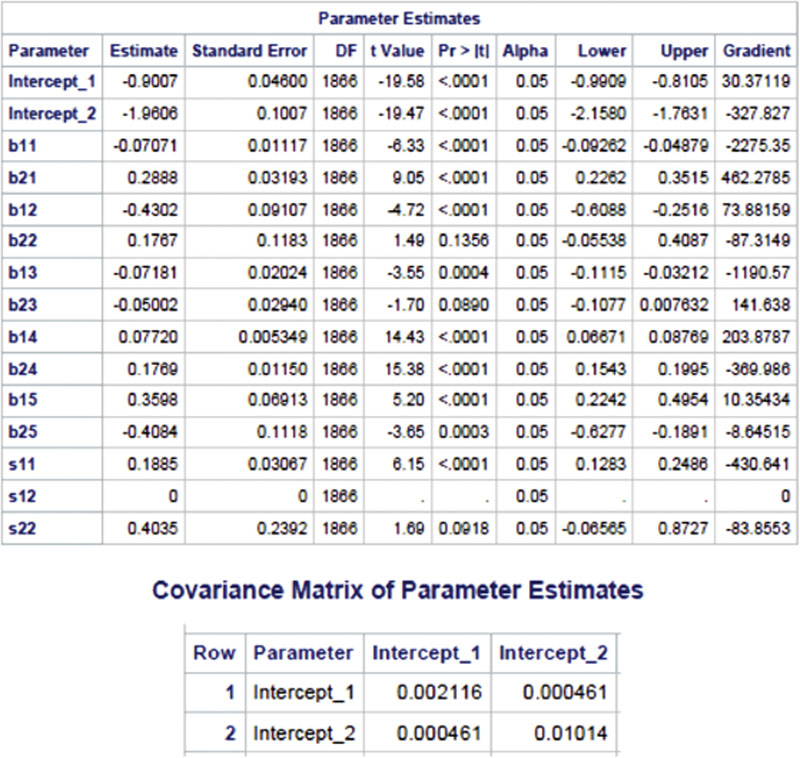
In SAS Program Output 11.1, the first table, “Parameter Estimates,” displays the estimates of the fixed and the random effects on the two logit components. For each parameter type, there are two estimates corresponding to the two logit components: log(P₁/P₂) and log(P₂/P₃), respectively. These results are consistent with those previously reported, thereby not being further interpreted. The second table, “Covariance Matrix of Parameter Estimates,” displays the local variance–covariance matrix of the intercepts on the two logit components needed to compute the variances and the covariance of the conditional effects of marital status on the health probabilities.

As indicated earlier, in the construct of the multinomial logit model, the regression coefficients of a covariate are not intuitive because they do not necessarily correspond to changes in a set of probabilities. Therefore, the estimated regression coefficients of marital status on the logit components need to be retransformed to the conditional effects on the probability scale to aid in the interpretation of the analytic results. With variable MARRIED being a dichotomous variable, Equations (11.25) and (11.27) are applied to generate the retransforms. First, using Equation (11.25) and the estimated regression coefficients reported in SAS Program Output 11.1, the baseline probability of disability and the death rate indicate the estimates for those currently not married (MARRIED = 0). In computing the probabilities at the fourth time (TIME = 6), the values of the three control variables need be held at sample means at the time point, and therefore, all five covariates are scaled at zero in the nonlinear predictions. Consequently, only the fixed and the random estimates for the intercepts need to be included for computing the two probabilities for those currently not married. Below is the computation of the two nonreference probabilities.

$\begin{array}{c}({\widehat{P}}_{10}\left|\text{time}=\right.6)=\frac{\text{exp}(-0.901)\exp \left[(0.189+0.002)/2\right]}{1+\text{exp}(-0.901)\exp \left[(0.189+0.002)/2\right]+\text{exp}(-1.961)\exp \left[(0.404+0.010)/2\right]}\\ =0\text{.254,}\end{array}$

$\begin{array}{c}({\widehat{P}}_{20}\left|\text{time}=\right.6)=\frac{\text{exp}(-1.961)\exp \left[(0.404+0.010)/2\right]}{1+\text{exp}(-0.901)\exp \left[(0.189+0.002)/2\right]+\text{exp}(-1.961)\exp \left[(0.404+0.010)/2\right]}\\ =0\text{.109,}\end{array}$

where $({\widehat{P}}_{10}\left|\text{time}=\right.6)$ is the predicted probability of disability at the fourth time, and $({\widehat{P}}_{20}\left|\text{time}=\right.6)$ is the death rate between the third and the fourth time points, for those currently not married. By definition, $({\widehat{P}}_{30}\left|\text{time}=6\right.)$, the probability of functional independence at the fourth time for those currently not married, is the residual to the sum of the two nonreference predictions, given by $({\widehat{P}}_{30}\left|\text{time}=6\right.)=1-0.254-0.109=0.637$.

Using Equations (11.28) and (11.29), the 2 × 2 variance–covariance matrix of the two predicted probabilities for those not currently married can then be computed. First, by using the analytic results reported in SAS Program Output 11.1 and Equation (11.28), the four elements in the B matrix are given by B₁₁ = 0.200, B₁₂ = B₂₁ = –0.029, and B₂₂ = 0.095, respectively. Let $V({\widehat{P}}_0\left|\text{time}=6\right.)$ denote the variance–covariance matrix for the predicted probabilities ${\widehat{P}}_1$ and ${\widehat{P}}_2$ at the fourth time point (time = 6) for those currently not married. Then, given the estimated variance–covariance matrix for the predicted multinomial logit components, the variance–covariance matrix for ${\widehat{P}}_1$ and ${\widehat{P}}_2$ at the fourth time point can be approximated by using Equation (11.29), given by

$\begin{array}{c}V({\widehat{P}}_0\left|\text{time}=6\right.)\approx \left(\begin{array}{l}0.200-0.029\\ -0.0290\text{.095}\end{array}\right)\left(\begin{array}{l}0.189+0.0020.001\\ 0.0010.404+0.010\end{array}\right){\left(\begin{array}{l}0.200-0.029\\ -0.0290\text{.095}\end{array}\right)}^{\prime }\\ =\left(\begin{array}{l}0.008-0.002\\ -0.0020\text{.004}\end{array}\right)\text{.}\end{array}$

The diagonal elements in the final matrix are the variance approximates for the two predicted probabilities at the fourth time for those currently not married, namely $\mathrm{var}({\widehat{P}}_{10}\left|\text{time}=\right.6)=0.008$ and $\mathrm{var}({\widehat{P}}_{20}\left|\text{time}=\right.6)=0.004$. Correspondingly, the square root of each variance estimate yields the approximate of the standard error for the predicted probability.

The computation for those currently married can be performed in the same fashion. First, a random intercept multinomial logit model is created by replacing the covariate MARRIED with a new variable UNMARRIED with 0 = currently married and 1 = currently not married. The SAS program for this model is exactly the same as SAS Program 11.5 except for the inclusion of UNMARRIED instead of MARRIED in covariates, and therefore, the program is not presented.

For those currently married, the predicted probability of disability at the fourth time is denoted by $({\widehat{P}}_{11}\left|\text{time}=\right.6)$ and the death rate between the third and the fourth time points is denoted by $\left({\widehat{P}}_{21}\left|\text{time}=\right.6\right)$. Following the same computational steps described earlier, the two nonreference health probabilities for those currently married are predicted as 0.262 and 0.111, respectively. As the residual estimate, the predicted probability of functional independence for those currently married at the fourth time is given by $({\widehat{P}}_{31}\left|\text{time}=6\right.)=1-0.262-0.111=0.626$. The variance estimates for the two nonreference predictions are 0.007 and 0.004, respectively. With the similarity of the computational steps described earlier, details about the computation for those currently married are not displayed. The reader might want to practice how the predicted probabilities and the $V({\widehat{P}}_1\left|\text{time}=6\right.)$ matrix are derived by following the computational steps for those currently not married.

Applying Equation (11.25), the conditional effects of marital status on the probability of disability and death rate at the fourth time are given by

$∆{\widehat{P}}_{\text{1,married}}={\widehat{P}}_{11}-{\widehat{P}}_{10}=0.262-0.276=-0.014\text{,}$

$∆{\widehat{P}}_{\text{2,married}}={\widehat{P}}_{21}-{\widehat{P}}_{20}=0.111-0.107=0.004\text{,}$

$∆{\widehat{P}}_{\text{3,married}}=-(∆{\widehat{P}}_{\text{1,married}}+∆{\widehat{P}}_{\text{2,married}})=-(-0.014+0.004)=0.010\text{.}$

Statistical significance of the conditional effects of marital status on the two nonreference predicted probabilities can be tested by using Equation (11.27). Specifically, the Wald chi-square statistics for the two conditional effects of marital status are computed as

$\begin{array}{l}{\chi }_{W\text{,}∆{\widehat{P}}_{\text{1, married}}}^2=\frac{{(0.262-0.276)}^2}{0.008+0.007-2\times \sqrt{0\text{.008}\times 0\text{.007}}}=2.963\text{,}\\ {\chi }_{W\text{,}∆{\widehat{P}}_{2,married}}^2=\frac{{(0.111-0.107)}^2}{0.004+0.004-2\times \sqrt{0\text{.004}\times 0\text{.004}}}=\mathrm{2.576.}\end{array}$

Each Wald statistic is distributed asymptotically as a chi-square with one degree of freedom under the null hypothesis. Therefore, given the Wald chi-square statistics, both the conditional effects of marital status are not statistically significant given α = 0.05. The evaluation of $∆{\widehat{P}}_3$, the residual effect, depends on the test results for the two nonreference conditional effects. Given the constraint that a set of conditional effects must sum up to zero, all three conditional effects of marital status at the fourth time point are considered statistically insignificant.

By applying the aforementioned computational procedure, the conditional effects of marital status and the corresponding variances at other time points can be predicted and computed. Table 11.3 displays the conditional effects of marital status on the probabilities of the two nonreference health states at all six time points.

Table 11.3

Conditional Effects of Current Marriage on Probabilities of Two Health States AHEAD Longitudinal Survey (N = 2000)

Functional Status	Time Point
	T0 (1998)	T1 (2000)	T2 (2002)	T3 (2004)	T4 (2006)	T5 (2008)
Disabled	−0.001	0.000	0.002	−0.013	−0.012	−0.003
	(0.030)	(0.143)	(0.017)	(2.963)	(1.032)	(9.655)
Dead	–	0.000	0.002	−0.013	−0.012	−0.003
		(0.230)	(0.698)	(2.576)	(1.096)	(0.500)

Note:    The conditional effects of marital status on the probability of functional independence depend on the testing results of the conditional effects on the probabilities of the two nonreference health states.

Table 11.3 displays that those currently married are slightly less likely than those currently not married to be functionally disabled and die. None of these conditional effects, except the one on the probability of disability at the sixth time, is statistically significant. Even that conditional effect, though statistically significant, is ignorable in analysis as it takes a value of −0.003, indicating a 0.3% difference between those currently married and those currently not married. Indeed, at the very old ages, survivors are those who are the most physically fit in the selection process, and as a result, group differences in health probabilities would gradually fade away, eventually displaying a homogeneous pattern.

The results shown in Table 11.3 provide very strong evidence that in longitudinal analysis on the multinomial response data, a strong fixed effect of a covariate on the logit scale does not necessarily translate into a strong, statistically meaningful impact on the probability scale. This is thought to be because the fixed effects on the logit scale are population-averaged without accounting for between-subjects variability, and in retransforming the fixed effects to the conditional effects on the probability scale, both between-subjects and within-subject variability is included, thereby substantially increasing the value of variance for the retransforms. Therefore, in the interpretation of the covariates’ effects on the multinomial longitudinal data, reliance on the fixed effects can result in misleading conclusions.

11.6.5. Graphical analysis on nonlinear predictions

To graphically display the statistical efficiency and coverage of different predicting approaches, Fig. 11.1 plots three sets of longitudinal trajectories on the probability of disability and the corresponding 95% confidence limits, with all covariates other than time fixed at time-specific sample means. These three sets of trajectories are derived from the retransformation method, the empirical BLUP, and the fixed-effects multinomial logit model, respectively. Each of these trajectory sets is compared to a solid growth curve and a shaded area representing an unbiased 95% confidence region from the full random intercept multinomial logit model.

In Panel a of Fig. 11.1, which compares the predicted pattern of change in the predicted probability of disability between the retransformation method and the full model, the two trajectory lines almost coincide in much of the observation period, thereby demonstrating the high efficiency and coverage of the retransformation method after a substantively important, statistically significant predictor is removed. The predicted trajectory curve in Panel b, obtained from the empirical BLUP, appears fairly close to the solid line; nevertheless, the two 95% confidence limit lines are much contracted as relative to the shaded area, highlighting the limited capability of the empirical BLUP to handle retransformation bias in nonlinear predictions. Panel c displays the predicted growth curve from the fixed-effects multinomial logit model, in which tremendous bias can be easily identified. In most time points, the dispersion of the predicted probability of disability is amiss: even the upper confidence limit of the probability is below the solid line.

Figure 11.2 plots three longitudinal trajectories of mortality and the corresponding 95% confidence limits, obtained from the retransformation method, the BLUP, and the fixed-effects multinomial logit model, respectively. The solid line and the shaded area in each panel are the growth curve and the 95% confidence region from the full random effects multinomial logit model, which are assumed to be exactly predicted for the convenience of evaluating the capacities of the three predicting methods. Panel a displays how well the retransformation method predicts the trajectory of the old-age mortality and the corresponding confidence limits, after one theoretically important, statistically significant predictor is removed. As shown in Panel b, the empirical BLUP predicts mortality fairly nicely, particularly at later time points, but the 95% confidence limits are considerably underestimated. In Panel c, the predicted trajectory curve of mortality is incorrect, with the two 95% confidence limits very narrowly scattered around the mean.

With inclusion of mortality as a competing risk, the pattern of change in the probability of disability differs tremendously from the pattern predicted by applying the mixed-effects binary logit model. As the mortality curve approximates a parallel line, the probability of disability does not display a distinctive pattern of change over time. Such an alteration in the predicted time trend provides very strong evidence that in the analysis of binary longitudinal health data among older persons, it is essential to take mortality as a competing risk; otherwise, longitudinal trajectories of health probabilities might be confounded tremendously by selection bias.

11.7. Summary