Search in book...
Toggle Font Controls
Create new playlist

Name your new playlist

Playlist description (optional)
Sign In

Email address

Password

Forgot Password?

or

Continue with Facebook

Continue with Google
Sign Up

Full Name

Email address

Confirm Email Address

Password

or

Continue with Facebook

Continue with Google

Chapter 7

Special topics on linear mixed models

Abstract

This chapter concerns several special topics in the application of linear mixed models. First, statistical models with adjustment of baseline response are described and discussed, in which the outcome variable is specified as a relative score rather than a score itself. The historical debate on the adjustment of baseline score is summarized for a two-point trend analysis. The Lord’s paradox, a classical example of the adjustment, is reviewed and discussed. The approach of adjusting the baseline response in longitudinal data analysis is then examined. Second, I present the statistical models adjusting misspecification of the normality hypothesis for the random effects, with an empirical illustration. Lastly, pattern-mixture modeling is delineated, both theoretically and with an empirical illustration. A variety of approaches are displayed to classify subjects into distinctive population groups representing profiled or heterogeneous patterns, and then followed by the specification of pattern-mixture modeling. Lastly, an empirical example is provided to display the application of pattern-mixture models in longitudinal data analysis.

Keywords

Gamma distribution

heterogeneity linear mixed model

heterogeneous population groups

Lord’s paradox

misspecification of normality hypothesis

pattern-mixture modeling

The aforementioned variety of linear mixed models has been widely applied in longitudinal data analysis. In certain situations, however, there is skepticism concerning the applicability of these models, particularly on the normality hypothesis for the distribution of the random effects. Corresponding to the raised questions, some advanced mixed-effects models have been proposed and used in longitudinal analyses. In some special occasions, those refined approaches are viewed as being preferable over the conventional linear mixed models.

In this chapter, several special topics are introduced in the analysis of normal longitudinal data. First, statistical models with adjustment of baseline response are described, in which the outcome variable is specified as a relative score rather than a score itself. Second, models adjusting misspecification of the normality hypothesis for the random effects are described and illustrated with an empirical example. Finally, I delineate pattern-mixture modeling, both theoretically and empirically.

7.1. Adjustment of baseline response in longitudinal data analysis

In longitudinal data analysis, the research focus is often on the time trend in the mean response and its differences across population subgroups of interest. The time trend reflects the pattern of change over time in the response variable originating from a specified time zero. As different population groups may have various score levels at baseline, a theoretical concern is sometimes advanced in trend analysis: Does the pattern of change over time in the mean response actually reflect an evolutionary process along the longitudinal course, or is it simply a function of the score level of the response at baseline? In analyzing longitudinal data of a randomized controlled clinical trial, there are often distinctive differences in the pattern of change over time in the health response between the treatment and the control groups. One possible argument is that if the two groups are associated with different mean scores at baseline, the subsequent differences can be the result of the discrepancies at baseline. Given such skepticism, a competing approach in longitudinal data analysis is to use the baseline response as a covariate. The rationale underlying this perspective is that by using the baseline score as a covariate, its confounding effect on the trajectory of individuals is addressed, and therefore, more reliable analytic results can be derived for the description of a time trend.

In this section, I first summarize the historical debate on the adjustment of baseline score for a two-point trend analysis. The Lord’s paradox, a classical example of the issue, is introduced and discussed. Next, the approach of adjusting the baseline response in longitudinal data analysis is examined. Lastly, I provide an empirical illustration, using the two longitudinal datasets described previously, to compare the results from different perspectives in the regard.

7.1.1. Adjustment of baseline score and the Lord’s paradox

Historically, there was much debate on the use of the baseline response as a covariate for a two-point pre–postanalysis. The argument concerns whether the baseline response should be adjusted, thereby deriving a relative change in the response at the follow-up. The classical work in this regard can be traced back to the 1960s when Lord (1967) provided an interesting example on the effect of the school diet on the students’ weights and the effect difference between boys and girls. As a typical pre–postanalysis, a student’s weight was measured twice, at the time of arrival in school and at nine months after arrival. In the example, Lord described two competing approaches to analyze the data. The first approach was to examine the change in the mean weight for boys and girls separately. Based on this approach, the mean weight was found to be identical for both sexes at the two time points. Thus, it was concluded from the results of this score change approach that on average, the school diet had no effect on the students’ weights, and there was no evidence that the diet had any differential effect on the two sexes.

The second approach Lord presented was an analysis of covariance (ANCOVA) perspective. By holding the initial weight equal for boys and girls, the regression lines displayed that boys gained more weight on average than girls. Therefore, it was concluded from this ANCOVA approach that the boys gained more weight than the girls between the two time occasions. Obviously, the conclusions from the two approaches are conflicting. This example is referred to as the Lord’s paradox.

To date, issues around the Lord’s paradox remain a topic of debate in longitudinal data analysis. With specific regard to the previous example, I consider the use of the first approach to be more appropriate because boys’ weights were generally more than girls’. In the second approach, the initial mean weights for the two sexes were subjectively held equal when comparing the change in the mean weight. As the weights at the second time occasion remained scatted in the empirical data, the boys, with their initial mean weight arbitrarily specified to be equal to the girls’, had to display a sharper increase in the mean weight to fit the data at the second time occasion. As a result, the second approach yielded an unrealistic pattern of change over time in students’ weights and an erroneous sex difference. Because the boys’ and the girls’ mean weights were supposed to differ at baseline, the school diet actually did not change the mean weight for both sexes.

The discussion on the second approach can be extended to the setting of a randomized controlled clinical trial on a normal health score. In the formulation of general linear models, an ANCOVA-type model, using the treatment factor (1 = treatment, 0 = control) and the baseline score as the covariates, can be written as

$Y_{i 2} = β_{0} + β_{1} Y_{i 1} + β_{2} Trea t_{i} + ɛ_{i},$

(7.1)

where Y_i1 is the response score for subject i at baseline, Y_i2 is the score for subject i at follow-up, and β₀ is the intercept indicating the expected response score at follow-up for the control group when

$Y_{i 1} = 0$

. The terms β₁ and β₂ are the regression coefficients of the baseline score and treatment on Y_i2, respectively, and ɛ_i is the error. The first regression coefficient, β₁, indicates the change in Y₂ with a one-unit increase in Y₁, and β₂ is the treatment effect on Y_i2 relative to a constant Y₁. Clearly, it is difficult to interpret both β₀ and β₁ substantively without further adjustments.

The first approach in the Lord’s paradox may be referred to as the change score approach because its application is based on the subtraction of the baseline response score from the follow-up score. This approach can be expressed as the pre–post difference in the response score, given by

$Y_{i 2} - Y_{i 1} = β_{0}^{*} + β_{2}^{*} Trea t_{i} + ɛ_{i}^{*},$

(7.2)

where the new intercept

$β_{0}^{*}$

represents the difference between

${\bar{Y}}_{1}$

and

${\bar{Y}}_{2}$

for the control group,

$β_{2}^{*}$

is the treatment effect on the pre–post difference in the response score, and

$ɛ_{i}^{*} = ɛ_{i 2} - ɛ_{i 1}$

. A closer look at Equation (7.2) suggests that the interpretation of the change score model is similar to that of the ANCOVA method, both displaying the effect of treatment on the difference between two scores. When

$β_{1} = 1$

, Equation (7.1) can be readily converted to Equation (7.2) by moving Y_i1 to the left side of the equation, and consequently, the interpretation of β₂ would be exactly the same as

$β_{2}^{*}$

. Even when β₁ differs from one, the interpretation of β₂ remains close to that of

$β_{2}^{*}$

because the baseline score and the assignment of treatments are theoretically irrelevant if randomization is implemented.

Given only two time points, a general linear model, like the OLS, can be applied to derive the regression coefficient estimates on the change score. Both approaches for adjusting the baseline score, the change score, and ANCOVA-type perspectives, have been criticized. Using the baseline score as a covariate can result in a lack of independence in residuals, thereby resulting in bias in parameter estimates. In certain situations, neglect of correlation between the baseline score and residuals can display a false conclusion on the significance of a covariate. The change score method is criticized for a lack of reliability and proneness to bias resulting from regression toward the mean. Allison (1990) compares the change score and the ANCOVA methods in different situations. He argues that each model has its own strengths and limitations, preferable to use under various circumstances. When the baseline response score has a causal effect on the follow-up score, it may be appropriate to use the baseline score as a control variable for correctly analyzing the effect of a treatment factor.

7.1.2. Adjustment of baseline score in longitudinal data analysis

In longitudinal data analysis, adjustment of the response score at baseline is simply an extension of the two-point perspective. Given more than two data points for each subject, the random effects or an appropriate residual variance–covariance structure are specified in linear regression models to account for intraindividual correlation. In terms of the ANCOVA-type model, the response score at baseline is used as a covariate, and consequently, interpretation of the regression coefficients for other covariates, including the intercept, is altered tremendously. Likewise, when a linear mixed model on the change score is specified, the regression coefficient of a covariate indicates the change in the response at follow-up time points relative to the baseline score, other covariates being equal. Questions may be advanced concerning the rationale of the relative change method. For example, does this approach derive better, more interpretable results than a conventional linear mixed model? And in which circumstances should the relative change method be applied in longitudinal data analysis?

Fitzmaurice et al. (2004) summarize four scenarios for modeling the baseline response score, denoted by Y₀, in the application of linear mixed models. These scenarios include (1) Y₀ is the baseline score included in the response vector Y as applied in conventional linear mixed models, with no assumption made about group differences in the mean response at baseline; (2) Y₀ is the baseline score included in the response vector Y as applied in conventional linear mixed models assuming the group means at baseline to be equal; (3) subtraction of Y₀ from each of the follow-up responses to form a set of relative response scores; and (4) Y₀ is used as a covariate in a linear mixed model on follow-up responses. In clinical experimental studies, randomization is usually designed to allocate subjects into two or more treatments prior to the start of the clinical trial. In analyzing data of randomized controlled clinical trials, it is appropriate to assume that the group response means at baseline are equal, and therefore, scenario (2) should be applied. Local tests on group differences in the response at each follow-up can then be routinely performed in the application of linear mixed models, as described in Chapter 5.

With regard to the analysis of data from clinical experimental studies, Fitzmaurice et al. (2004) advance an interesting proposition. As clinical trials are usually not implemented until after the origin of the study time, treatment should not have a main effect in regression modeling (in linear regression models, the main effect of treatment indicates the effect of treatment at baseline). Therefore, only the interaction term between treatment and time needs to be specified. This proposition makes strong theoretical sense because a medical treatment cannot exert any actual impact on the response before the experimentation is implemented. Statistically, however, removing the main effect of a covariate from the estimating process will not affect the derivation of other parameter estimates, the model fit, and model-based predictions as long as that covariate is included in the specified interaction term.

It is also contended that in the analysis of data from randomized controlled clinical trials, the use of the third and the fourth scenarios affects the statistical efficiency of parameter estimates and leads to difficulty in interpreting the analytic results. Furthermore, a subject whose baseline response is missing but information at follow-ups is available is included in the estimation of parameters for the conventional linear mixed model; this subject, however, is excluded in the use of the change score or the ANCOVA-type approaches. Consequently, the quality of parameter estimates will be affected by applying the third or the fourth scenarios if missing data on the baseline response are substantial.

In the analysis of longitudinal data from observational surveys, there is no randomization implemented, and therefore, the researcher should not make the assumption that the mean response at baseline is equal across different population subgroups. In these situations, the significance test on group differences in repeated measurements of the response should include the contrast at baseline, which corresponds to the first scenario. Consequently, the first scenario is appropriate to apply. As indicated in Chapter 5, group differences in the response at baseline and at the follow-ups can be estimated and statistically tested by the specification of the

$\tilde{L}$

vectors. The use of the first scenario has the added advantage that subjects with any information of the response at any time point are all included in fitting linear mixed models.

Given the previous discussions, the application of the third or the four scenarios, the score change, and the ANCOVA-type models is generally not recommended in longitudinal data analysis. By using those relative score methods, the interpretation of analytic results becomes inexplicit, and the parameter estimates cannot be used to predict the pattern of change over time in the response without further adjustments. For example, in the application of the ANCOVA-type method, the baseline response is used as a covariate, and correspondingly, the intercept represents the expected response score at the first follow-up time point when the baseline score and all other covariates are scaled zero. Here, consider the case of the PCL score: What does it mean for a PCL score of 0? Furthermore, this coefficient cannot convert to the score change relative to the baseline unless the regression coefficient of the baseline score is one.

Indeed, in longitudinal data analysis, it is important to specify the baseline score as a component of Y. The baseline response is the starting point to portray a time trend; it is an integral part of the pattern of change over time in the response and its group differences. It is also important to include as much information as possible in the analysis of longitudinal events, particularly for studies based on a small sample size. Occasionally, the ANCOVA-type method is applied in nonlinear mixed models, in which the stochastic processes in the post state given a prior status are modeled to predict transition probabilities. In such situations, the prior status is often specified as a covariate in a nonlinear mixed model. This type of nonlinear modeling techniques will be described in Chapter 12.

7.1.3. Empirical illustrations on adjustment of baseline score

To illustrate the change score and the ANCOVA-type approaches, I continue the use of the two datasets previously indicated: one from a randomized controlled clinical trial and one from a large-scale observational survey. The objective of the present illustrations is to compare the analytic results from three different perspectives to handle the baseline response: the conventional linear mixed model, the ANCOVA-type approach using the baseline score as a covariate, and the change score method. From the different sets of analytic results, the three perspectives can be compared and examined effectively.

First, I reanalyze the effectiveness of acupuncture treatment on the PCL score. As indicated earlier, in the design of a typical randomized controlled clinical trial, a medical treatment cannot have an effect on the health score before the treatment protocol is formally implemented. Correspondingly, given the baseline time point scaled at 0, acupuncture treatment does not have a main effect. Below is the SAS program for constructing a linear mixed model on the PCL score without specifying the main effect of acupuncture treatment.

SAS Program 7.1a:

In SAS Program 7.1a, the main effect of acupuncture treatment is not specified in the MODEL statement. As will be displayed below, however, the analytic results remain the same, with or without the specification of the main effect of the treatment factor.

The other two linear mixed models, using the response score at baseline as a covariate and defining the change score as the dependent variable, can be programmed by adapting the preceding SAS program. The SAS program for these two models is displayed below.

SAS Program 7.1b:

In SAS Program 7.1b, I create two revised PCL variables in the DATA step. The first revised PCL variable, retaining the name PCL_SUM, only has three data points without including the baseline time. The second revised PCL variable, named PCL_DIFF, also with three data points, is created as the subtraction of the baseline PCL score from each of the PCL scores measured at the follow-ups. In the first linear mixed model, the variable PCL_SUM0 is specified as a covariate on the PCL scores at the three follow-up time points, other specifications being the same as previously specified. The second linear mixed model uses PCL_DIFF as the dependent variable in the MODEL statement, other specifications being equal to those indicated previously. In both models, the TIME(REF = “1”) option in the CLASS statement informs SAS that TIME = 1 be used as the reference level for TIME. A portion of the analytic results from SAS Programs 7.1a and 7.1b, including the fixed effects and the −2 log-likelihood ratio statistics, are displayed in Table 7.1.

Table 7.1

Fixed Effects of Three Linear Mixed Models: (A) Without a Main Effect for Treatment, (B) Baseline PCL Score Used as a Covariate, and (C) Change Score Approach

Explanatory Variable	Parameter Estimate	Standard Error	Degrees of Freedom	t-Value	p-Value
	Model Without the Main Effect of Treatment (−2 LL = 1384.9; p < 0.0001)
Intercept	55.444	2.560	54	21.66	<0.0001
Time 1	−3.963	2.103	127	−1.88	0.0618
Time 2	−2.976	2.218	127	−1.34	0.1821
Time 3	−9.234	2.186	127	−4.22	<0.0001
Treat × time 1	−14.496	3.075	127	−4.71	<0.0001
Treat × time 2	−15.808	3.305	127	−4.78	<0.0001
Treat × time 3	−8.669	3.250	127	−2.67	0.0086
	Model Using PCL at Baseline as a Covariate (−2 LL = 960.9; p < 0.0001)
Intercept	12.537	6.893	47	1.82	0.0753
PCL at time 0	0.702	0.118	47	5.95	<0.0001
Treatment	−13.639	3.189	47	−4.28	<0.0001
Time 2	0.728	2.039	80	0.36	0.7221
Time 3	−5.277	2.008	80	−2.63	0.0103
Treat × time 2	−0.875	3.070	80	−0.28	0.7764
Treat × time 3	−5.796	3.016	80	1.92	0.0582
	Change Score Model (−2 LL = 964.5; p < 0.0001)
Intercept	−3.963	2.250	48	−1.76	0.0845
Treatment	−14.037	3.317	48	−4.23	0.0001
Time 2	0.635	2.040	80	0.31	0.7564
Time 3	−5.221	2.009	80	−2.60	0.0111
Treat × time 2	−0.693	3.072	80	−0.23	0.8222
Treat × time 3	−5.901	3.018	80	1.96	0.0541

The first panel in Table 7.1 displays the analytic results from the conventional linear mixed model without specifying the main effect of acupuncture treatment. Both the fixed effects and the model fit statistics are exactly the same as those reported in SAS Program Outputs 5.1 and 5.2. The only difference is a one-unit loss in the degrees of freedom in the model without the main effect of treatment. The results of the random component, not presented in the table, are also identical. Clearly, although it is theoretically constructive, saving the specification of the main effect of the treatment factor in linear mixed models makes no statistical differences in parameter estimates, both the fixed and the random.

In the second model of Table 7.1, where PCL score at baseline is used as a covariate, acupuncture treatment displays a statistically significant effect on reduction in the PCL score at the second time point (−13.639, p < 0.0001) with Time 1 being the reference but not on the scores at the third and the fourth time points. This effect pattern is consistent with the results from the conventional linear mixed model. The regression coefficient of the baseline PCL score, 0.702 and statistically significant, indicates a 0.7-points addition to the PCL score at follow-ups per one-unit increase in PCL_SUM at baseline, other variables being equal. Clearly, in this model the intercept does not have a substantively meaningful interpretation. The results of the Type 3 tests on the fixed effect, not included in Table 7.1, present that the overall effects of the baseline PCL and acupuncture treatment are statistically significant on the PCL score at the follow-ups. Using PCL_SUM0 as the control variable, neither the overall effect of time nor of the interaction between time and treatment is statistically significant.

With the baseline PCL score being adjusted, the results do not display a time trend and its group differences. The intercept does not indicate the score difference between the baseline and the first follow-up because the regression coefficient of PCL_SUM0 is not one. Nevertheless, the fixed-effect estimates can be used to predict the PCL score at each time point and for each treatment group. For example, the predicted PCL score for those in the control group at the second time point can be computed as 12.537 + 0.702 × (baseline PCL). Similarly, for those receiving acupuncture treatment at the same time point, the PCL score is 12.537 + 0.702 × (baseline PCL) – 13.639. Compared to the direct interpretation of the regression coefficients from the conventional linear mixed model, the additional computation is clearly inconvenient.

The third model reported in Table 7.1 is a modified version of the second model, as discussed earlier. The interpretation of the dependent variable in this model is the change in the PCL score at a follow-up time point relative to the score at baseline, thereby reflecting the same kind of change in the response score as displayed in the second model. As a result, the two sets of analytic results, including the fixed effects, the model fit statistics, and the random effects, not presented, share some similarities. The intercept in the third model, −3.963, is the estimated difference in the PCL score between the baseline and the second time points for the control group. Although linear predictions can be computed from the fixed-effect estimates, as is applied for the ANCOVA-type model, the additional computation is inconvenient compared to a direct interpretation of the results from a conventional linear mixed model.

Obviously, the specifications of the above three models do not improve the statistical efficiency, coverage, and interpretability in analyzing the effect of acupuncture treatment on the PCL score, as compared to the results from the conventional linear mixed model. Neither do they facilitate a better portrayal of a time trend. In particular, the results from the second and the third models can potentially confuse our understanding of the pattern of change over time and its group differences in the PCL score.

To further examine the issue, next I perform the same comparative procedure to analyze the longitudinal trajectory of the ADL count and its difference between those currently married and those currently not married among older Americans. It is not adequate to apply the first model presented in Table 7.1 for the AHEAD longitudinal data. While acupuncture treatment has yet to be implemented at Time 0, an older person is associated with a marital status at the start of the AHEAD survey. Therefore, the linear mixed model used in Chapter 5 is reapplied first, followed by the application of the two relative score models. As the basic syntax is identical to that of SAS Program 7.1, except for a different number of time points and a different set of variables, the SAS program for this example is not displayed. The following table summarizes a portion of the analytic results from the three linear mixed models on the ADL count.

In Table 7.2, the first panel displays the results of the conventional linear mixed model, also reported in SAS Program Output 5.4. The second model uses the baseline ADL count as a covariate, with its regression coefficient being 0.724 and statistically significant. Analytically, this estimated regression coefficient indicates the change in the ADL count at follow-up time points given a one-unit increase in the baseline count, other variables being equal. Substantively, this effect displays a positive relationship between the baseline PCL count and the subsequent count values. The intercept, 0.387, is the ADL count at the second time point (TIME = 1) when the ADL count at baseline is scaled 0, which does not translate into a substantively meaningful interpretation. The regression coefficient of marital status is 0.031, suggesting that those currently married are expected to have an ADL count that is 0.031 points higher than those currently not married at the second time point. This main effect of marital status, however, is not statistically significant.

Table 7.2

Fixed Effects of Three Linear Mixed Models: (A) Conventional Specifications, (B) Baseline ADL Count Used as a Covariate, and (C) Change Score Approach

Explanatory Variable	Parameter Estimate	Standard Error	Degrees of Freedom	t-Value	p-Value
	Model With Full Specifications (−2 LL = 20,087.7; p < 0.0001)
Intercept	0.673	0.044	1726	15.29	<0.0001
Married	0.029	0.059	300	0.49	0.6218
Time 1	0.257	0.036	4814	7.18	<0.0001
Time 2	0.513	0.052	4814	9.86	<0.0001
Time 3	0.579	0.058	4814	9.93	<0.0001
Time 4	0.768	0.061	4814	12.55	<0.0001
Time 5	0.932	0.060	4814	15.58	<0.0001
Mar. × time 1	−0.159	0.053	4814	−3.01	0.0026
Mar. × time 2	−0.252	0.078	4814	−3.23	0.0012
Mar. × time 3	−0.233	0.090	4814	−2.58	0.0099
Mar. × time 4	−0.060	0.098	4814	−0.61	0.5438
Mar. × time 5	−0.309	0.101	4814	−3.07	0.0021
	Model Using AD at Baseline as a Covariate (−2 LL = 14,499.0; p < 0.0001)
Intercept	0.387	0.046	1423	8.50	<0.0001
ADL_0	0.724	0.028	1423	26.16	<0.0001
Married	0.031	0.064	212	0.49	0.6240
Time 2	0.336	0.044	3384	7.64	<0.0001
Time 3	0.446	0.055	3384	8.09	<0.0001
Time 4	0.660	0.060	3384	10.93	<0.0001
Time 5	0.851	0.059	3384	14.32	<0.0001
Mar. × time 2	−0.145	0.068	3384	−2.14	0.0326
Mar. × time 3	−0.157	0.088	3384	−1.79	0.0735
Mar. × time 4	−0.005	0.098	3384	−0.05	0.9615
Mar. × time 5	−0.275	0.101	3384	−2.71	0.0067
	Change Score Model (−2 LL = 14,589.1; p < 0.0001)
Intercept	0.238	0.044	1424	5.42	<0.0001
Married	0.056	0.064	212	0.87	0.3837
Time 2	0.348	0.044	3384	7.90	<0.0001
Time 3	0.480	0.055	3384	8.71	<0.0001
Time 4	0.710	0.060	3384	11.77	<0.0001
Time 5	0.895	0.059	3384	15.05	<0.0001
Mar. × time 2	−0.151	0.068	3384	−2.22	0.0266
Mar. × time 3	−0.177	0.088	3384	−2.02	0.0435
Mar. × time 4	−0.036	0.098	3384	−0.36	0.7156
Mar. × time 5	−0.303	0.101	3384	−2.99	0.0028

Given the fixed-effect estimates, the ADL count at each time point for each marital status group can be predicted by the computational formulas described earlier. For example, the predicted ADL count for those currently not married at the second time point is computed as 0.387 + 0.724 × (baseline ADL_COUNT), other covariates being held at zero. Similarly, for those currently married at the same time, the prediction is 0.387 + 0.724 × (baseline ADL_COUNT) + 0.031. In this computation, the estimate of the baseline ADL count can be borrowed from the intercept of the first model.

The regression coefficients of time from the third model can be interpreted as the difference in the ADL count between a given follow-up time point and the baseline, which is somewhat similar to the interpretation for the second model. As a result, the two sets of analytic results, including the fixed effects, the model fit statistics, and the random effects (not presented in Table 7.2), are close to each other. The intercept for the third model, 0.238, is the estimated difference in the ADL count between the baseline and the second time point for those currently not married. While linear predictions of the ADL count can be computed from the fixed-effect estimates, the additional calculation is unnecessary because the classical linear mixed model can derive linear predictions directly by the application of least squares means. Indeed, the use of the relative-score methods does not yield direct, meaningful interpretations regarding the time trend and its group differences in the ADL count.

It may be summarized from the previous two examples that the two relative score methods, the ANCOVA-type and the change score, do not yield the analytic results as efficiently, explicitly, and reader-friendly as the conventional approach. The fixed effects in the relative score models present indirect effects on repeated measurements of the response, some being hard to interpret substantively without further adjustments. Although interpretable results and unbiased linear predictions can be obtained from additional computations, it is really unnecessary to generate interpretable results by transforming the indirect effects. Furthermore, the baseline response score is included in every step of estimation in the application of the relative score methods, and therefore, subjects with the baseline measurement missing but with some information available at follow-ups will all be excluded from the estimating process. Consequently, the application of both the ANCOVA-type and the change score approaches reduces statistical efficiency as well as causes problems of interpretability in the analytic results. Caution must apply, therefore, when using the relative change models in longitudinal data analysis.

7.2. Misspecification of the assumed distribution of random effects

In linear mixed models, the between-subjects random effects are generally assumed to be normally districted with mean 0 and covariance matrix G. All parameters, fixed or random, are estimated given this normality hypothesis. Statisticians tend to take it for granted that the between-subjects random effects, specified to account for unobserved heterogeneity, potentially correspond to the large sample property. When the desirable large-sample behavior follows, as is usually the case in the analysis of large-scale survey data, this specification for the distribution of the random effects yields statistically efficient, consistent, and robust parameter estimates. This practical perspective seems not unreasonable in general situations. As they essentially represent the impact of some unspecified and unrecognizable factors on the response, the normality hypothesis on the distribution of the random effects should be supported by large-sample theory. Given this belief, the empirical Bayes estimates for the random effects are heavily dependent on the normality assumption. Empirically, however, this hypothesis cannot always hold in some special situations. The violation of the normality assumption for the random effects can adversely affect the validity and reliability of parameter estimates, both the fixed and the random.

More recently, there has been increasing skepticism toward the normality hypothesis in approximating the random effects. In survival analysis, some scientists attempt to model unobserved heterogeneity by defining a quantity termed “frailty,” a convenient notion used most frequently by mathematical biologists and demographers (Hougaard, 1986; Vaupel et al., 1979). Frailty may refer to a broad range of dimensions, such as genetic predisposition, physiological senescence parameters, economic capability, family history of diseases, and the like (Hougaard, 1995; Manton et al., 1994; Vaupel et al., 1979). In the frailty theory, individuals in a random sample have different levels of frailty, and the frailer ones tend to die sooner than the others, other covariates being equal. Because survival is selected systematically by the unobserved frailty factor, the true distribution of the random effects may deviate gradually from a normal distribution over time (Vaupel et al., 1979). If this phenomenon occurs, more advanced statistical models and methods need to be applied to address the misspecification of the normality hypothesis in the random effects.

In this section, several statistical approaches are described that address the violation of the normality hypothesis on the random effects. I first describe the heterogeneous linear mixed model developed by Verbeke and Lesaffre (1996) and then delineate a modified linear mixed model with the specification of a nonnormal, parametric distribution for the random effects. Third, I introduce a work that evaluates and analyzes the behavior of the best linear unbiased prediction of the random effects under different assumptions. An empirical illustration is provided to compare model-based least squares means and the BLUPs.

7.2.1. Heterogeneity linear mixed model

The specification of linear mixed models depends regularly on the normality hypothesis for the random effects, both marginally and conditionally. Verbeke and Lesaffre (1996) contend that local normality of the random effects for a section of data does not necessarily result in a normal distribution in the entire population. When subjects are classified into a finite number of distinctive groups based on certain longitudinal profiles, a mixture of conditional normal distributions of the random effects for those profiled groups can lead to nonnormality of the marginal distribution. A heterogeneity linear mixed model is proposed to address the misspecification of the normality hypothesis.

Let subjects be divided into K heterogeneous population groups, with mean vectors of the random effects

${\tilde{μ}}_{k}$

and covariance matrices G_k, where k = 1,…, K. The vector b_i can then be expressed in terms of a mixture of K q-dimensional normal distributions with mean vectors

${\tilde{μ}}_{k}$

and covariance matrices G_k, given by

$b_{i} = \sum_{k = 1}^{K} p_{k} N ({\tilde{μ}}_{k}, G_{k}),$

(7.3)

where p_k is the weight for group k with properties

$\begin{array}{l} \sum_{k = 1}^{K} p_{k} = 1, \\ \sum_{k = 1}^{K} p_{k} {\tilde{μ}}_{k} = 0. \end{array}$

The second property of p_k is a necessary constraint leading to the upholding of the linear predictor

$E (y_{i}) = X_{i}^{'} β$

Let δ_ik be a status indicator such that

$δ_{i k} = 1$

if b_i is sampled from group k in the mixture and

$δ_{i k} = 0$

if b_i is sampled from other groups. Given a mixture of K normal distributions, the overall covariance matrix of the random effects is then given by

$\begin{array}{l} \tilde{G} = var [E (b_{i} |δ_{i 1}, ...., δ_{i K})] + E [var (b_{i} |δ_{i 1}, ...., δ_{i K})] \\ = var (\sum_{k = 1}^{K} {\tilde{μ}}_{k} δ_{i k}) + E (\sum_{k = 1}^{K} G_{k} δ_{i k}) \\ = \sum_{k = 1}^{K} p_{k} {\tilde{μ}}_{k} {\tilde{μ}}_{k}^{'} + \sum_{k = 1}^{K} p_{k} G_{k} . \end{array}$

(7.4)

To avoid numeric problems, it is assumed that G_k = G for all k’s and

$b_{1}, ...., b_{N}$

are mutually independent. Given these assumptions, a heterogeneous linear mixed model can be specified as follows:

$\{\begin{cases} Y_{i} |b_{i} \sim N (X_{i}^{'} β + Z_{i}^{'} b_{i}, R_{i}), \\ b_{i} |\tilde{μ} \sim N (\tilde{μ}, G), \\ \tilde{μ} \in ({\tilde{μ}}_{1}, ...., {\tilde{μ}}_{K}) . \end{cases}$

$\tilde{μ}$

is not identically zero, the assumption

$b_{i} \sim N (0, G)$

is relaxed, thereby allowing heterogeneity for the mean of the random-effects distribution. Given the construction of heterogeneous groups, which will be discussed in Section 7.3, this heterogeneity model can be regarded as a hierarchical empirical Bayes model, with the marginal distribution of the measurements being written as

$Y_{i} \sim \sum_{k = 1}^{K} p_{k} N (X_{i}^{'} β + Z_{i}^{'} {\tilde{μ}}_{k}, V_{i}) .$

(7.5)

The terms β,

${\tilde{μ}}_{k}$

, p_k, and parameters in V_i can be estimated by using the maximum likelihood estimator. Operationally, either the NR or the EM algorithm can be applied to derive the fixed and the covariance parameter estimates. For more details concerning this heterogeneity linear mixed model, the reader is referred to Verbeke and Lesaffre (1996) and Verbeke and Molenberghs (2000, Chapter 12).

7.2.2. Nonnormal random effect distribution in linear mixed models

The previous heterogeneity linear mixed model is proposed to account for unobserved heterogeneity in the random effects by replacing a normal distribution with a finite mixture of normals (Agresti et al., 2004). The application of this approach results in a sizable addition of parameters, thereby further complicating the already complex structure in longitudinal data. With the added parameters, the heterogeneity model is more suitable for the analysis of large-scale survey data than for the study of clinical experimental data generally characterized by small sample sizes.

Some researchers attempt to estimate the patient-specific repeated measurements of health scores from a different direction (Zhang et al., 2008). Specifically, Zhang et al. (2008) find the distribution of the random effects to be negatively skewed, and accordingly, they modify the conventional linear random coefficient model by specifying a nonnormal distribution for the random effects. Let

$b_{i} = \tilde{R} {\tilde{s}}_{i}$

, where

$\tilde{R}$

is a 2 × 2 matrix for covariance

$\tilde{r}$

between the random intercepts and the random slopes of time with diagonal elements taking value one, and

${\tilde{s}}_{i}$

is the component of the random effects that are independent. The linear random coefficient model is then given by

$y_{i} = X_{i}^{'} β + Z_{i}^{'} \tilde{R} {\tilde{s}}_{i} + ɛ_{i},$

(7.6)

where

$Z_{i} = (1_{n_{i}}, T_{i})$

$1_{n_{i}}$

is an n_i-dimensional design vector of all ones, and T_i is the vector for time components. The random slopes contained in

${\tilde{s}}_{i}$

are assumed to be i.i.d. log-gamma distributed for addressing skewness across different groups. By such a modification, the standard linear random coefficient model can be applied with normal intercepts and log-gamma distributed slopes. Consequently, the negative skewness in the distribution of the random slopes is accounted for in this parametric mixed model. For analytic convenience, the number of groups is specified as two in the following presentation.

The maximum likelihood estimator can be applied to find parameter estimates in the log-gamma linear mixed model. Two groups are specified in the study with the first group having N₁ and the second group N₂ = N − N₁ subjects. The vector

${\tilde{s}}_{i} = {({\tilde{s}}_{i 1}, {\tilde{s}}_{i 0})}^{'}$

9 contains the independent components of the random intercepts and the random slopes for subject i. Accordingly, the likelihood function is given by

$L (θ) = \prod_{k = 1}^{2} \prod_{i = 1}^{N_{k}} \int [\int φ (y_{i} |{\tilde{s}}_{i}) ϕ ({\tilde{s}}_{i 0}) d {\tilde{s}}_{i 0}] f_{k} ({\tilde{s}}_{i 1}) d {\tilde{s}}_{i 1},$

(7.7)

where θ is the parameter vector consisting of both the fixed and the random components,

$φ (\cdot)$

denotes the normal density of Equation (7.6), and

$f_{k} (\cdot)$

is the log-gamma density for group k (k = 1, 2).

After some simplification, the log-likelihood function is

$l (θ) = \sum_{k = 1}^{2} \sum_{i = 1}^{N_{k}} \log \int \tilde{g} ({\tilde{s}}_{i 1}) f_{k} ({\tilde{s}}_{i 1}) d {\tilde{s}}_{i 1} d {\tilde{s}}_{i 1},$

(7.8)

where

$\tilde{g} ({\tilde{s}}_{i 1}) = \frac{\exp \{- {[y_{i} - X_{i}^{'} β - {\tilde{s}}_{i 1} (T_{i} + \tilde{r})]}^{'} W_{i} [y_{i} - X_{i}^{'} β - {\tilde{s}}_{i 1} (T_{i} + \tilde{r})]\}}{{(2 π σ)}^{n_{i} / 2} \sqrt{(σ + n_{i} \tilde{τ}) / σ}},$

and

$\tilde{τ}$

is the i.i.d. variance of

${\tilde{s}}_{i 0}$

, and

$W_{i} = \frac{1}{2 σ} I_{n} - \frac{\tilde{τ}}{2 σ (σ + n_{i} \tilde{τ})} J_{n},$

with I_n being the n_i-dimensional identity matrix and

$J_{n} = I_{n} I_{n}^{'}$

Statistically, the estimating procedure for this nonnormal linear mixed model is difficult as the likelihood for the model has no closed form expressions due to integration of a nonnormal distribution of the random effects. A variety of numeric methods, however, can be applied to approximate the parameters. For example, by using Gaussian quadrature, which will be described in Chapter 8, the MLE of the fixed and the random parameters, contained in

$\hat{θ}$

, can be adequately obtained.

According to Bayesian inference, misspecification of an assumed distribution of the random effects results in a misspecified predictive distribution given the observed data (Box and Tiao, 1973). This misspecification, in turn, yields an erroneous expectation of the posterior predictive distribution, thereby leading to bias in linear predictions. In the model with the log-gamma distributed random slopes of time, the conditional mean predictors of the

${\tilde{s}}_{i}$

components are given by

${\hat{\tilde{s}}}_{i j} = \frac{\int {\tilde{s}}_{i j} f (y_{i} |{\tilde{s}}_{i}) f ({\tilde{s}}_{i}) d {\tilde{s}}_{i}}{\int f (y_{i} |{\tilde{s}}_{i}) f ({\tilde{s}}_{i}) d \tilde{s}}, j = 1,2,$

(7.9)

where the integrals can be evaluated by the application of the adaptive Gaussian quadrature described in Chapter 8. The predictors of b can then be calculated based on the estimate of

$\tilde{r}$

and the predictors of

${\tilde{s}}_{i}$

The conditional mean predictor in the log-gamma linear mixed model is considered to yield a smaller mean square error than the conventional predictor (Zhang et al., 2008). An analog to the likelihood ratio test statistic is also developed to test the statistical significance of a direct contrast of predictions between the conventional and the log-gamma linear mixed models. For details concerning this test statistic, the reader is referred to the original article displaying the model (Zhang et al., 2008). The log-gamma distributed random coefficient model can be adapted into a log-gamma distributed random intercept perspective if the random intercepts are found to be skewed.

7.2.3. Best predicted random effects in different distributions

The conventional linear mixed models assume normality for the random effects. Given this hypothesis, the predictive distribution of the random effects for subject i given y_i is multivariate normal. In the construct of linear mixed models, the mean of such a conditional distribution minimizes the mean square error of the prediction, thereby referred to as the best linear unbiased prediction or BLUP. The rationale and detailed specifications of BLUPs are provided in Chapter 4.

McCulloch and Neuhaus (2011) conducted a series of simulations aimed at evaluating the behavior of predictions for the random effects in linear and generalized mixed models given different assumptions. The focus of the analysis is on the prediction of the values of b_i with the minimum mean square error predicted values. For a scalar b_i, for example, such a minimum mean square error of prediction can be mathematically expressed as

${\tilde{b}}_{i} \equiv E (b_{i} |Y) ≔ \min E [{(b_{i} - b^{*})}^{2}],$

(7.10)

where

${\tilde{b}}_{i}$

is termed the best predicted value, or BP, of b_i, and b^* is the true value of the random effect scalar.

For the linear random intercept model with

$b_{i} \sim i.i.d. F_{b}$

, where

$E (b_{i}) = 0$

and

$var (b_{i}) = σ_{b}^{2}$

, the BP values can be expressed in terms of a Bayes model, given by

$\begin{array}{l} {\tilde{b}}_{i} = E (b_{i} |Y_{i}) \\ = E (b_{i} |{\bar{Y}}_{i .}) \\ = \frac{\int_{- \infty}^{\infty} b_{i} f_{{\bar{Y}}_{i .} |b_{i}} ({\bar{Y}}_{i .} |b_{i}) f_{b_{i}} (b_{i}) d b_{i}}{\int_{- \infty}^{\infty} f_{{\bar{Y}}_{i .} |b_{i}} ({\bar{Y}}_{i .} |b_{i}) f_{b_{i}} (b_{i}) d b_{i}} \\ = \frac{\int_{- \infty}^{\infty} b_{i} \exp [- \frac{n_{i}}{2 σ_{ɛ}^{2}} {({\bar{Y}}_{i .} - {\bar{X}}_{i}^{'} β - b_{i})}^{2}] f_{b_{i}} (b_{i}) (b_{i}) d b_{i}}{\int_{- \infty}^{\infty} \exp [- \frac{n_{i}}{2 σ_{ɛ}^{2}} {({\bar{Y}}_{i .} - {\bar{X}}_{i}^{'} β - b_{i})}^{2}] f_{b_{i}} (b_{i}) (b_{i}) d b_{i}} . \end{array}$

(7.11)

Given the earlier specification, McCulloch and Neuhaus (2011) explore the behavior of

${\tilde{b}}_{i}$

in four different distributions for

$f_{b_{i}}$

, which are scaled to have standard deviation σ_b. The four distributions are: (1) Gaussian, (2) a skewed and truncated distribution, (3) a heavy-tailed distribution, and (4) a mixture of two Gaussian distributions. Those distributions are believed to represent a wide variety of distributions for the random effects.

For the general Gaussian distribution, assuming known values of

$σ_{b}^{2}$

$σ_{ɛ}^{2}$

, and β, the BP value of b_i can be written as

$\begin{array}{l} {\tilde{b}}_{i} = E (b_{i} |Y) \\ = \frac{σ_{b}^{2}}{σ_{b}^{2} + σ_{ε}^{2} / n_{i}} ({\bar{Y}}_{i} - {\bar{x}}_{i}^{'} β) . \end{array}$

(7.12)

The BP value of b_i is equivalent to the

$BLUP ({\hat{b}}_{i})$

, described in Chapter 4. After some simplification, Equation (7.12) can further reduce to

$\begin{array}{l} {\tilde{b}}_{i} = \frac{σ_{b}^{2}}{σ_{b}^{2} + σ_{ɛ}^{2} / n_{i}} (b_{i} - ɛ_{i .}) \\ = {\tilde{λ}}_{i} (b_{i} - ɛ_{i .}), \end{array}$

(7.13)

where

${\tilde{λ}}_{i} = σ_{b}^{2} / (σ_{b}^{2} + σ_{ɛ}^{2} / n_{i})$

is the classical shrinkage factor in the BLUP predictor in linear mixed models, also described in Chapter 4.

The performance of

${\tilde{b}}_{i}$

can then be evaluated effectively by considering the conditional distribution of

${\tilde{b}}_{i}$

given b_i. If the assumed distribution for b_i is Gaussian, the conditional distribution of

${\tilde{b}}_{i}$

can be expressed as

${\tilde{b}}_{i} |b_{i} \sim indep. N ({\tilde{λ}}_{i} b_{i}, {\tilde{λ}}_{i}^{2} σ_{ɛ}^{2} / n_{i}) .$

(7.14)

Given Equation (7.14), McCulloch and Neuhaus (2011) summarize a number of properties for

${\tilde{b}}_{i}$

•

${\tilde{b}}_{i}$

is conditionally biased toward 0 by the shrinkage factor

${\tilde{λ}}_{i}$

; accordingly, the predictor

${\hat{y}}_{i}$

is shrunk toward the grand mean

$X_{i}^{'} β$

• The conditional bias and the variance tend to zero as

$σ_{b}^{2} n_{i} / σ_{ɛ}^{2} \to \infty$

• The distribution of

${\tilde{b}}_{i}$

converges to the distribution of b_i as

$n_{i} \to \infty$

• Irrespective of the true distribution of b_i, the unconditional distribution of

${\tilde{b}}_{i}$

has mean zero and variance equal to

${\tilde{λ}}_{i} σ_{b}^{2}$

• The variance of

${\tilde{b}}_{i}$

is smaller than the variance of b_i by the shrinkage factor

${\tilde{λ}}_{i}$

; that is,

$var ({\tilde{b}}_{i}) \neq G$

Given the assumed Gaussian distribution of the random effects and using certain numeric methods, the true distribution of

${\tilde{b}}_{i}$

can be evaluated for the aforementioned four distributions. After a series of simulations on empirical data, a number of important implications follow. First, the distributions of best-predicted values for the random effects are highly dependent on the assumed distribution and hence are not reliable indicators of the distribution for the random effects. Second, very different distributions for best-predicted values can perform similarly in practice, as gauged by the overall mean square error of prediction. Third, distributions of the random effects that may be statistically better fitting may not perform better in the overall prediction. These findings lead to the conclusion that misspecification of the assumed distribution for the random effects affects prediction of the random effects but not the prediction of the response.

According to the results from the series of analyses, McCulloch and Neuhaus (2011) suggest that although the predictions themselves can be sensitive to the assumed distribution of the random effects, the overall accuracy of the prediction is little affected for mid-to-moderate violation of the assumptions. Therefore, the standard linear mixed models, assuming the Gaussian distributed random effects, usually result in good performance of the best-predicted values across a wide variety of situations with different true random effect distributions. These findings thus indicate that the linear mixed-effects regression procedures available in various statistical software packages are highly applicable for dealing with different distributions in longitudinal data analysis. Only in some special cases does the violation of the normality hypothesis for the random effects result in severely biased linear predictions. In Chapter 14, this issue will be further explored when some newly advanced techniques are presented.

7.2.4. Empirical illustration: comparison between BLUP and least squares means

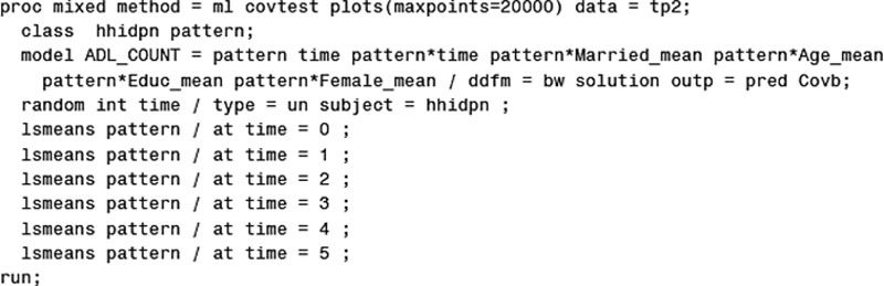
In this section, I evaluate the behaviors of three sets of the predicted values for the response variable, derived from the least square means, the BLUPs, and a linear mixed model with the random intercepts assumed to have a log-gamma distribution, respectively. Because a large sample size is required to conduct such an exploratory analysis, the AHEAD longitudinal data are used for this illustration. ADL_COUNT remains the dependent variable, measured at six time points: 1998, 2000, 2002, 2004, 2006, and 2008. There are two operational objectives in this analysis. The first goal is to analyze whether there are distinctive differences in the ADL predictions and the corresponding standard errors between the least squares means and the empirical BLUPs. The second goal is to examine whether the specification of the log-gamma-distributed random effect fits the data significantly better than the classical linear mixed model, using the model chi-square criterion. For analytic convenience and simplicity, the linear random intercept model is applied by modifying the linear random coefficient model specified in Chapter 4 (Section 4.6.2). The maximum likelihood estimator is applied to find parameter estimates due to the convenience of comparing the model fit statistics across different regression models. Slightly different from previous AHEAD analyses, in this illustration marital status is specified as one of the predictor variables on the mean ADL count for the entire population. Therefore, the variable Married is rescaled to be centered at the mean, named Married_mean. The three previously used centered variables – Age_mean, Educ_mean, and Female_mean – are still included in the regression as predictors. Additionally, the interaction between marital status and time is removed in this exploratory analysis.

The least squares means are computed first at the six time points. As indicated in Chapter 5, for the linear random intercept model, the least squares means can be computed at the exact times by using the ESTIMATE statement in the SAS PROC MIXED procedure. The following is the SAS program for this analysis.

SAS Program 7.2:

SAS Program 7.2 first creates four time-specific centered predictors, including the centered variable Married_mean. Given the GROUP BY TIME option in the PROC SQL statement, centering is applied at each time point, rather than relative to the entire sample, to predict a population grand mean of the ADL count. The RANDOM statement only includes INT, thereby specifying a linear random intercept linear model. I then request SAS to compute the least squares means at six exact times by using the ESTIMATE statement in the PROC MIXED procedure. In performing this calculation, the values of all the predictors not listed in the ESTIMATE statement are held at sample means, as default in SAS.

Next, the empirical BLUPs of the ADL count are derived. As indicated in Chapter 4, to compute the empirical BLUP value of the ADL count for a hypothetical population, a scoring dataset needs to be created. In the scoring dataset, ADL_COUNT is specified as missing and the values of the predictors as sample means to yield the predictions corresponding to the least squares means. Combining the scoring dataset with the empirical data does not have any impact on the estimation and the approximation of the parameters. After the parameter estimates or approximates are obtained, each observation, including those in the scoring dataset, has a predicted value of the ADL count given the predictors’ values, the estimated regression coefficients, and the predicted subject-specific random effect. Below is the SAS program for creating the scoring dataset.

SAS Program 7.3a:

In SAS Program 7.3a, the scoring dataset is created by keeping the ID and TIME variables from the original AHEAD dataset and specifying ADL_COUNT = . and the four-centered predictors = 0 in the hypothetical data. The DATA TP3 step combines the observed and the scoring datasets into one. The SAS program for the regression part is presented below.

SAS Program 7.3b:

In SAS Program 7.3b, the PROC MIXED procedure is similar to that of SAS Program 4.3a. The temporary dataset PRED is sorted by time. Lastly, the mean ADL count is computed at each exact time for the scoring data set, manipulated by the WHERE ADL_COUNT = . AND MARRIED_MEAN = 0 AND AGE_MEAN = 0 AND EDUC_MEAN = 0 AND FEMALE_MEAN = 0” statement. By doing so, the time-specific ADL means can be predicted for the entire population and then be compared with predictions from other methods.

The third step is to fit a linear random intercept linear model assuming a log-gamma distribution for the random intercepts. To perform this analysis, some additional conditions need to be specified. Let

${\bar{θ}}_{1}$

and

${\bar{θ}}_{2}$

be the variances of the scale parameter

$\overset{⌢}{λ}$

and the shape parameters

$\overset{⌢}{k}$

in the specification of the gamma distribution. The density function of the gamma distribution then becomes

$f (b_{i} |{\bar{θ}}_{1}, {\bar{θ}}_{2}) = \frac{{b_{i}}^{1 / {\bar{θ}}_{1} - 1} \exp (- b_{i} / {\bar{θ}}_{2})}{Γ (1 / {\bar{θ}}_{1}) {\bar{θ}}_{2}^{1 / {\bar{θ}}_{1}}} .$

(7.15)

For analytic convenience and identifiability, the mean of b’s is set at 1, given the condition that

$\overset{⌢}{λ} = \overset{⌢}{k}$

thus

${\bar{θ}}_{2} = {\bar{θ}}_{1} = 1 / \overset{⌢}{k}$

. It follows then that Equation (7.15) reduces to

$f (b_{i} |{\bar{θ}}_{1}) = \frac{{b_{i}}^{1 / {\bar{θ}}_{1} - 1} \exp (- b_{i} / {\bar{θ}}_{1})}{Γ (1 / {\bar{θ}}_{1}) {\bar{θ}}_{1}^{1 / {\bar{θ}}_{1}}},$

(7.16)

where the parameter

${\bar{θ}}_{1}$

measures the degree of intraindividual correlation in the presence of the predictors and the specified random effects, with a greater value highlighting a higher correlation among repeated measurements of the response for the same subject.

Given the specification of a nonnormal distribution for the random intercepts, the PROC NLMIXED procedure in SAS is applied to yield parameter estimates for the third model. In SAS, the PROC NLMIXED procedure only allows a single random effect with a normal distribution, and accordingly, I adapt the method of the probability integral transformation, recommended by Nelson et al. (2006), to fit the model with a log-gamma distributed random effect. Specifically, the gamma random effect b_i can be obtained from a set of transformations: (1) α_i ∼ N(0, 1), (2) p_i = Φ(α_i), (3)

$b_{i 2} = F_{{\bar{θ}}_{1}}^{- 1} (p_{i})$

, and (4)

$z_{i} = \bar{θ} b_{i 21}$

, where

$F_{{\bar{θ}}_{1}}^{- 1} (.)$

is the inverse c.d.f. of the gamma distribution, and Φ(.) is the standard normal c.d.f. (the probit function). Given these steps of transformation, a linear random intercept model with log-gamma distributed random intercepts can be conducted using the following SAS program.

SAS Program 7.4:

In SAS Program 7.4, a nonlinear procedure is applied to specify a linear mixed model with a nonlinear distribution of the random intercepts. In the PROC NLMIXED statement, the MTHOD = GAUSS option calls for the application of the Gaussian quadrature, NOAD requests that the Gaussian quadrature be nonadaptive, FD specifies that all derivatives be computed using finite difference approximations, and qpoints = 3 tells SAS that three quadrature points be used in each dimension of the random intercepts. In applying this technique, the number of quadrature points can be increased or decreased as desired. In principle, a higher number of quadrature points improve the accuracy of the approximation; in the meantime, it increases the computational burden. The detailed inference of the technique will be described extensively in the Chapter 8.

From the previous three SAS programs, three sets of linear predictions of the ADL count are produced from the least squares means, the empirical BLUPs, and the linear random intercept model assuming the random intercepts to follow a log-gamma distribution, respectively. The results are summarized in Table 7.3.

Table 7.3

Three Sets of Linear Predictions for ADL Count at Six Time Points: From Least-Squares Means, Empirical BLUP, and Model With a Log-Gamma Distribution

Time (T_j)	Least Square Means (χ² = 20,535.1)		BLUP (χ² = 20,535.1)		Log-gamma (χ² = 832E15)
Time (T_j)	Prediction	SE	Prediction	SE	Prediction	SE
0	0.6766	0.0312	0.6766	0.0196	0.9351	0.0033
1	0.8580	0.0292	0.8580	0.0196	1.1436	0.0033
2	1.0393	0.0291	1.0393	0.0196	1.3521	0.0033
3	1.2707	0.0312	1.2707	0.0196	1.5606	0.0033
4	1.4021	0.0349	1.4021	0.0196	1.7691	0.0033
5	1.5835	0.0398	1.5835	0.0196	1.9776	0.0033

Table 7.3 displays the increasing trend over time in the ADL count in older Americans, consistent across all three sets of predictions. As the least squares means and the empirical BLUPs are derived from the same regression model, the first two sets of predictions are associated with the same model chi-square value (−2 log-likelihood). The third set of predictions comes from the linear random intercept model assuming log-gamma distributed random intercepts, associated with an exceptionally high-model chi-square value. According to the statistical criterion that less is better with regard to the value of −2(LLR), the model with the log-gamma distributed random intercepts is shown to lose important statistical information, thereby being not statistically efficient as compared to the other two mixed models. The largely elevated value of −2(LLR) is a typical indication of model misspecification. Therefore, I cannot reject the null hypothesis that the integration of a log-gamma distributed term for the random effects does not significantly improve the estimating quality of the linear mixed model. Neither can the predictions from this model be accepted given much elevated predicted values. Given these results, further explorations are based on the first two sets of ADL_COUNT predictions.

Given the specification of the linear random intercept model, the predicted ADL values from the least squares means and the empirical BLUPs are exactly the same at each of the six times. The standard errors estimated for the BLUPs, however, are considerably lower than those from the least squares means. As indicated earlier,

${\tilde{b}}_{i}$

is conditionally biased toward 0 by the shrinkage factor

${\tilde{λ}}_{i}$

, and therefore, the empirical BLUPs are shrunk toward the grand mean

$X_{i}^{'} β$

. Given the specification of a single term for the random effects, the between-subjects covariance structure is CS; as a result, the BLUP prediction has a constant value of the standard error approximate throughout all times. On the other hand, the least squares means approach generates the predicted population margins over a balanced population based on the model, assuming the normality hypothesis for the random intercepts to be valid.

When the random coefficient approach is applied, the least squares means and the empirical BLUPs on the ADL count still produce the same predictions of the response for the entire population. Table 7.4 displays two sets of the ADL predictions by specifying both the random intercepts and the random coefficients of time.

Table 7.4

Predicted Values for ADL Count at Six Times: From Least Squares Means and BLUP

Time (T_j)	Least Square Means (χ² = 19,910.3)		BLUP (χ² = 19,910.3)
Time (T_j)	Prediction	Standard Error	Prediction	Standard Error
0	0.6352	0.0303	0.6352	0.0201
1	0.8783	0.0291	0.8783	0.0207
2	1.1214	0.0333	1.1214	0.0224
3	1.3645	0.0412	1.3645	0.0251
4	1.6076	0.0511	1.6076	0.0285
5	1.8507	0.0621	1.8507	0.0324

Table 7.4 displays that the random coefficient model fits the longitudinal data significantly better than the random intercept model, given the significant reduction in the value of model chi-square. Compared to the predictions reported in Table 7.3, however, there are only some minor changes in both the predicted values and the standard error estimates. Given the addition of a random term, the empirical BLUP standard errors are no longer constant while remaining much lower than those generated from the least squares means. The face values of the predictions remain exactly the same for the two predictors thanks to the property that E(b) = E(BLUP b) = 0 and E(e) = 0 . In linear predictions for specific population subgroups, the two sets of predictions can depart considerably given the different assumptions of data structures: balanced versus unbalanced.

In empirical research, whether to report the result of predictions from the empirical BLUPs or from the least squares means depends on the researcher’s judgment on the nature of a longitudinal dataset and one’s understanding of the missing-data mechanism in longitudinal data. For example, if missing observations are not sizable in a large-scale dataset, the least square means approach is preferable because the large sample behavior usually follows in large-scale survey data. On the other hand, if there are a large number of missing observations and/or the researcher has skepticism on the normality assumption for the random effects, the empirical BLUP results should be reported.

In the present analysis, using either set of the predicting results generates about the same conclusions, although there are considerable differences in the standard error estimates. This relative consistence is usually the case in the application of linear mixed models. In nonlinear predictions, the model-based and the empirical BLUPs can yield very different nonlinear predictions, both for the means and for the standard errors. This discrepancy in nonlinear predictions is thought to be because complex procedures of data transformation and retransformation are involved in nonlinear predictions, and ignorance of any component in nonlinear predictions can result in a sizable prediction bias. In Chapters 8–12, I will further discuss the issues concerning nonlinear predictions when describing various nonlinear mixed-effects models and their estimating procedures.

7.3. Pattern-mixture modeling

In Section 7.2, I described a variety of refined linear mixed models that propose to correct misspecification of the normality hypothesis for the random effects, including the heterogeneity model. Corresponding to the heterogeneity mixed modeling, one of the remarkable progresses in handling heterogeneous normality is the advancement of pattern-mixture models in longitudinal data analysis. Pattern-mixture modeling was originally developed in missing data analysis (Diggle and Kenward, 1994; Glynn et al., 1986; Little, 1993, 1994a, 1995; Little and Rubin, 2002). Given its high applicability for analyzing longitudinal data with strong selection effect, pattern-mixture modeling has been extended to the analyses of other types of heterogeneous patterns.

This section concerns the description and the application of pattern-mixture models. I first present a variety of approaches for classifying subjects into distinctive population groups representing profiled or heterogeneous patterns. Next, pattern-mixture modeling is specified and discussed. Lastly, an empirical example is provided to display the application of pattern-mixture models in longitudinal data analysis.

7.3.1. Classification of heterogeneous groups

In longitudinal data analysis, classification of heterogeneous groups originates from missing-data analysis. As indicated in Chapter 1, missing data can be classified into various missing-data patterns. According to impact on the response variable, missing data can be divided into “completely at random” (MCAR), “missing at random” (MAR), and “missing not at random” (MNAR) mechanisms (Diggle and Kenward, 1994; Little, 1995; Little and Rubin, 2002; Robins et al., 1995; Rubin, 1976, 1987), as mentioned previously. Likewise, given the frequency and ordering of missing data, missing data can be categorized into monotone, nonmonotone, and some other patterns. With a variety of classification standards for missing-data patterns, subjects can be organized into a number of heterogeneous groups. For example, monotone or nonmonotone, missing earlier or missing late, and random or nonrandom can all serve as the criteria to classify subjects. As Chapter 14 is entirely devoted to missing-data analyses, the detailed missing-data classification and the associated mathematical definitions are not further discussed in this section.

A natural extension of missing-data classification is categorization of subjects according to survival status and the timing of death among those deceased (Dufouil et al., 2004). For adults, survival reflects a selection of the fittest process. Individuals in a random sample are assumed to have different levels of frailty, and the frailer ones tend to die sooner than the others. Because the frailty factor is usually unobservable, the true stochastic process of repeated measurements for a population may be masked as a consequence of continued changes in population health composition (Vaupel et al., 1979). Selection eliminates less fit individuals from a given cohort as its age increases. Consequently, the mortality rate for an old cohort increases less rapidly with age than it would otherwise because the surviving members of the cohort are the ones who are the most fit and less disabled (Christensen et al., 2008). Therefore, in performing a longitudinal data analysis for older persons, it is empirically practical to regard survival status at each follow-up time point as a reasonable factor for classifying subjects into different mixture components. In different situations, the classification of mixture population groups can also be conducted by other factors displaying distinctively heterogeneous patterns of distributions in a population. For example, a random sample of patients with depressive symptoms can be classified into heterogeneous health groups by the number of medical conditions.

The classification of heterogeneous mixture patterns can also be performed by applying certain statistical criteria. For example, heterogeneous patterns can be statistically recognized by the use of linear discriminant analysis (LDA). The formulation of this method shares some common properties with both ANOVA and factor analysis but with different analytic focus. Specifically, LDA is designed to model the difference between distinctive classes of data based on the correlated measurements, and therefore, an observational vector y can be assigned to one of the K groups by following certain statistical criteria. A common unstructured covariance matrix is generally assumed for all population classes. The classical LDA approach requires complete data for all observations, thereby forcing removal of all the individuals with missing observations in longitudinal data.

Tomasko et al. (1999) extend the classical LDA to the random-effects regression models. In this innovative method, the correlated measurements are modeled by using a structural covariance in the discriminant function. It is concluded that the inclusion of the random-effects covariance structure results in improvement in precision, particularly in the analyses based on small samples. For more details concerning LDA and its applications in longitudinal data analysis, the reader is referred to McLachlan (2004), McLachlan and Basford (1988), and Tomasko et al. (1999).

Some scientists extend the conventional pattern-mixture perspectives by applying latent growth mixture modeling (LGMM) to identify heterogeneous patterns. This approach specifies latent classes, rather than observable classes of subjects, which can be identified and estimated as hypothetical subpopulations given observed data (Muthén and Shedden, 1999; Muthén, 2001). In LGMM, the distribution of the observed responses is modeled through mixed-growth trajectories. Each subpopulation is specified to have its own model parameter values, and consequently, the distribution of the observed outcomes is viewed as a mixture distribution (Muthén, 2001). When individual variations are assumed to only occur between groups, the LGMM becomes the latent growth curve model (LGCM), in which each observation is subject to a probability to belong to each latent class (Muthén, 2001). The latent factor classification approaches will be described and discussed in Chapter 13, and therefore, they are not further elaborated in this chapter.

7.3.2. Basic theory of pattern-mixture modeling

Given the classification of subjects into a number of heterogeneous groups, the pattern-mixture model can be created by the specification of joint modeling that combines different patterns into a unifying estimating process. In the original work of this analysis, Rubin (1976) formalizes models for the missing-data mechanisms by introducing a stochastic missing-data indicator matrix, denoted by

$\overset{⌢}{M}$

. While the definition of

$\overset{⌢}{M}$

in the context of missing data analysis is described in Chapter 14, in this section the notation

$\overset{⌢}{R}$

is used to indicate a broader concept of heterogeneous patterns. Given the discussions in Section 7.3.1, the matrix

$\overset{⌢}{R}$

represents any set of distinctive mixture groups, with missing-data patterns being a special case.

Let

$\overset{⌢}{R} = ({\overset{⌢}{R}}_{1}, ...., {\overset{⌢}{R}}_{N})$

be the associated random vector of a pattern indicator variable, where each

${\overset{⌢}{R}}_{i}$

(i = 1, 2,…, N) takes a value ranging from 1 to K to indicate a specific pattern. The probability that

$\overset{⌢}{R}$

takes the value

$\overset{⌢}{r} = ({\overset{⌢}{r}}_{1}, ...., {\overset{⌢}{r}}_{N})$

is defined as

$g_{\overset{⌢}{φ}} (\overset{⌢}{r} |\overset{⌢}{ϕ})$

, where the vector

$\overset{⌢}{ϕ}$

is specified to indicate parameters for the pattern selection. In the longitudinal setting, inference of pattern-mixture models starts with the full data density, given by

$f (y_{i}, {\overset{⌢}{r}}_{i} |X_{i}, Z_{i}, \overset{⌢}{θ}, \overset{⌢}{ϕ}),$

where

$\overset{⌢}{θ}$

and

$\overset{⌢}{ϕ}$

are the measurement and pattern-selection process vectors that parameterize the joint distribution.

The classical pattern-mixture model is based on the application of factorization, given by

$f (y_{i}, {\overset{⌢}{r}}_{i} |X_{i}, Z_{i}, \overset{⌢}{θ}, \overset{⌢}{ϕ}) = f (y_{i} |{\overset{⌢}{r}}_{i}, X_{i}, Z_{i}, \overset{⌢}{θ}) f ({\overset{⌢}{r}}_{i} |X_{i}, \overset{⌢}{ϕ}),$

(7.17)

where the first component on the right of the equation is the density of the observed data that depends on different heterogeneous patterns and the second the density of a heterogeneous group itself. Therefore, as

$\overset{⌢}{R}$

indicates different patterns given a specific heterogeneity classification, Equation (7.17) is marginally a mixture of different populations characterized by the observed pattern. Consequently, observed data can represent identifiable subpopulations according to a number of heterogeneous or mixture patterns, with each subpopulation having its own model parameter values. The pattern-specific parameters can be estimated by the application of the maximum or the restricted maximum likelihood estimator. Correspondingly, for subject i the longitudinal outcome mean can be viewed as a weighted average of mean values associated with a variety of mixture patterns (Verbeke and Molenberghs, 2000), with the sum of weights being one.

7.3.3. Pattern-mixture model

For analytic simplicity, in the following presentation, subjects are classified into a number of groups according to one’s dropout status at time point j, where j = 1,…, n. Given this classification standard, a classical pattern-mixture model is proposed given a monotone missing-data pattern. Correspondingly, the pattern indicator vector

$\overset{⌢}{R}$

takes values 1,…, n (in this context, K = n) with element

${\overset{⌢}{R}}_{i}$

indicating a specific time point at which subject i’s last observation occurs. With the specification of

${\overset{⌢}{R}}_{i}$

, the full data for subject i is written as

$y_{i} = {(y_{i 1}, ..., y_{i {\overset{⌢}{R}}_{i}})}^{'}$

. The weight for each mixture pattern, denoted by w_k where k = 1,…, n, can be either obtained from the observed data or approximated by the estimated probability of a specific pattern from a logistic or a multinomial logit regression model (Little and Wang, 1996; Verbeke and Molenberghs, 2000).

Given the individual pattern indicator

${\overset{⌢}{R}}_{i}$

, the conditional distribution of the response for subject i can be expressed as

$y_{i} |{\overset{⌢}{R}}_{i} \sim N [μ_{i} ({\overset{⌢}{R}}_{i}), Σ_{i} ({\overset{⌢}{R}}_{i})],$

(7.18)

where

$μ_{i} ({\overset{⌢}{R}}_{i})$

is a n_i × 1 mean vector of the response and

$Σ_{i} ({\overset{⌢}{R}}_{i})$

is the n_i × n_i residual variance–covariance matrix. Let all vectors of

$μ_{i} ({\overset{⌢}{R}}_{i})$

be combined into µ. It follows that for pattern k, where

$k = 1,2,..., n$

, the combined mean vector can be written as

$μ (k) = [\begin{array}{c} μ_{1} (k) \\ ⋮ \\ μ_{n} (k) \end{array}] and Σ (k) = [\begin{array}{c} σ_{11} (k) & \dots & σ_{1 n} (k) \\ ⋮ & ⋱ & ⋮ \\ σ_{n 1} (k) & \dots & σ_{n n} (k) \end{array}] .$

where

$μ_{j} (k)$

is the conditional mean of the response at time point j (j = 1, …, n) combining all members belonging to pattern k.

With the conditional mean of the response, the marginal distribution of the response can be expressed in terms of a mixture of n normal distributions with mean vector

$μ = \sum_{k = 1}^{K} w_{k} μ (k),$

where

$μ = {(μ_{1}, μ_{2}, ..., μ_{n})}^{'}$

is a vector of n marginal means with each element expressed as a weighted mean across K patterns. Specifically, in the construct of the pattern-mixture model, the marginal mean of the response at time point j is given by

$μ_{j} = \sum_{k = 1}^{K} w_{k} μ_{j} (k), for j = 1,..., n .$

The variance–covariance matrix of µ can be obtained by applying the delta method, with a detailed description of the method provided in Appendix B.

Empirically, with the inclusion of covariates and the random effects, the earlier pattern-mixture model can be formulated in the framework of linear mixed models. For subject i given the individual pattern indicator

${\overset{⌢}{R}}_{i}$

, the pattern-mixture model can be written as

$Y_{i} = X_{i}^{'} β ({\overset{⌢}{R}}_{i}) + Z_{i}^{'} b_{i} + e_{i},$

(7.19)

where

$\begin{array}{l} b_{i} \sim N [0, G ({\overset{⌢}{R}}_{i})], \\ e_{i} \sim N [0, Σ_{i} ({\overset{⌢}{R}}_{i})] . \end{array}$

The previous pattern-mixture model cannot be fully identified without making further restrictions on the conditional distribution because there are no data to identify

$μ (k)$

and the corresponding residual variance–covariance parameters for missing cases at time point k (in this case, k = 1,…, n). For solving this issue, researchers have contributed a variety of approaches for identifying parameters for missing cases. Little (1993) recommended the use of complete case missing values as parameter restrictions, borrowing the set of observed components in the completers beyond time point k to set a conditional density of unobserved components. Molenberghs et al. (1998), on the other hand, proposed to borrow the conditional distributions from those dropping out after the time point k to identify those dropping out at k. Both of these restrictions correspond to the MAR hypothesis. From a different perspective, Rubin (1977) proposes sensitivity analysis on differences in the mean and the variance–covariance parameters for various patterns.

In empirical analyses, pattern-specific parameter estimates in pattern-mixture modeling can be derived either by creating K separate linear mixed models for each heterogeneous pattern or by specifying a unifying mixed model that includes all pattern-specific parameters within an integrated inference. The latter approach is statistically more efficient but may be associated with serious numeric problems in the identification of a high number of heterogeneous patterns. In these situations, the researcher can assume a common variance–covariance matrix of the random effects for all mixture patterns, given by

$G (k) = G$

. By doing so, numeric problems can often be avoided with a reduction in the size of parameters. The assumption of a common covariance structure for heterogeneous groups can be tested by specifying two pattern-mixture models: one assuming heterogeneous covariance structures and one with a common covariance matrix. As follows, a sensitivity analysis can be performed on the changes in the fixed effects and the model fit statistic.

Another concern that sometimes arises in the application of pattern-mixture modeling is the specification of weights for K heterogeneous patterns. For example, using the timing of death as the classification criterion makes strong practical sense in aging and health studies, particularly since high mortality is often the primary reason for dropout among older persons. In the classical pattern-mixture model, the density of a heterogeneous group is assumed to be constant over time given the classification of subjects at baseline. When subjects are categorized according to survival status and the timing of death, it does not seem reasonable to include the deceased in the prediction of marginal means because they no longer possess any actual values or characteristics to predict. Correspondingly, the pattern-specific weight w_k should be a moving function of time, and accordingly, the marginal distribution of weights for each heterogeneous pattern varies with the elimination of deaths.

With respect to this issue, a competing hypothesis is that those deceased can be regarded as representing a sample that is randomly drawn from the distribution of a dropout population at a given time, and therefore, the model-based predictions for the dead may be viewed as the unbiased measurements of the outcome for the general dropouts. The resulting mixture then represents an “immortal cohort” (Dufouil et al., 2004). This immortal cohort hypothesis, however, does not reflect the reality of longitudinal processes in which death is an integral, unavoidable component.

7.3.4. Empirical illustration of pattern-mixture modeling

This illustration is a follow-up analysis to the example presented in Section 7.2.4. Pattern-mixture modeling is applied to analyze the AHEAD longitudinal data. The operational objective is to compare the ADL predictions from a pattern-mixture model with the least squares means from the conventional linear mixed model. In older persons, those deceased at different times or ages are heterogeneous in terms of health status and disabilities given the selection process. According to frailty theory, mortality eliminates less fit individuals from a given cohort, and the older persons who die early are generally those who are less fit than the others. Therefore, older persons deceased in various time intervals represent a number of heterogeneous health groups.

Accordingly, in this analysis older persons are categorized into six heterogeneous groups: (1) the subjects who died prior to the start of the second AHEAD wave (2000), (2) the subjects deceased between the second and the third time points (2000–2002), (3) deceased between the third and the fourth time points (2002–2004), (4) deceased between the forth and the fifth time points (2004–2006), (5) deceased between the fifth and the sixth time points (2006–2008), and (6) those alive at the time of the sixth time point. Given this classification, the analysis is aimed at examining the following propositions. First, those deceased earlier are expected to have a higher ADL count at baseline than those deceased later. Second, those deceased earlier are expected to experience a sharper increase over time in the ADL count than those deceased later. Third, those who have survived throughout all six waves are expected to have the lowest ADL count and the lowest rate of ADL increase over time among all six health groups.

In the application of the pattern-mixture model, the variable PATTERN is defined as a classification factor with six levels, with the sixth level used as the reference. The random coefficient linear model is applied to yield parameter estimates for all patterns, with PATTERN, TIME, and the four centered variables (Married_mean, Age_mean, Educ_mean, and Female_mean) included as the predictors on the ADL count. Each pattern is assumed to have its own parameter values, and therefore, an interaction between PATTERN and each of the other predictors is created. The following is the SAS program for the pattern-mixture model.

SAS Program 7.5a:

In SAS Program 7.5a, first the variable PATTERN is created according to the previous classification. Except for the inclusion of PATTERN and its interactions with the other predictors, this SAS program is analogous to a regular PROC MIXED procedure, assuming all heterogeneous patterns to be subject to a common variance–covariance matrix for the random effects. If the shape of the time trend is found to differ significantly across heterogeneous groups, not the case in this analysis, the quadratic time (and cubic if necessary) component and some three-way interactions should be created to reflect the additional source of variability.

SAS Program 7.5a produces a large amount of analytic results. The value of model chi-square for the pattern-mixture model is 18,585.7, significantly lower than 19,910.3 from the linear random coefficient model (see Table 7.4). Therefore, the specification of this pattern-mixture model fits the AHEAD data significantly better than the classical, single-pattern perspective. The following output table displays the solution for the fixed effects of the variables PATTERN, TIME, and their interaction terms.

SAS Program Output 7.1a:

All the fixed effects of PATTERN, TIME, and the corresponding interaction terms are statistically significant. Given the statistical significance of the interaction between TIME and PATTERN 5, the main effect of PATTERN 5 is also statistically significant. The results of Type 3 tests of the fixed effects, not presented, display that all the overall fixed effects are statistically significant. The fixed effects of the other four predictor variables, all statistically significant, are not of direct interest and thus are not presented.

The random effect approximates and the corresponding standard errors for the pattern-mixture model are presented in the following output table.

SAS Program Output 7.1b:

According to the previous table, the variance estimate of within-subject random errors

$σ_{ɛ}^{2}$

is 0.58 (p < 0.0001), identical to the estimated residual variance from the conventional linear mixed model. All three covariance parameter estimates for the random effects are statistically significant, with p-values all smaller than 0.01. The unstructured (2 × 2) variance–covariance matrix of the random effects, assumed to be common across all heterogeneous groups, is given by

$G = (\begin{array}{c} 0.933 & - 0.058 \\ - 0.058 & 0.103 \end{array}) .$

With the earlier variance–covariance matrix, the variance estimates of the random effects for the intercept and the slope of time are 0.933 and 0.103, respectively, somewhat different from those from the one-pattern model. Covariance of the two random effects is −0.058, displaying a negative but weak association. These test results are asymptotically valid given the large sample size of the AHEAD data.

Given the fixed-effect estimates and a common variance–covariance structure for the random effects, the least squares means can be computed to display a mixture of time trends in the ADL count for various heterogeneous patterns. The following SAS program is created for this step.

SAS Program 7.5b:

In SAS Program 7.5b, I ask SAS to compute the least squares means at six exact times for each heterogeneous group. Given the specification of six patterns, the program yields a lengthy output table of the least squares means and the corresponding standard errors, which are summarized in Table 7.5.

Table 7.5

Predicted Means of ADL Count and Standard Errors for Six Patterns and at Six Exact Times: Pattern-Mixture Model for Older Americans (N = 1718)

Time	Pattern
Time	1	2	3	4	5	6
0	1.75 (0.10)	0.69 (0.09)	0.62 (0.10)	0.43 (0.09)	0.07 (0.09)	0.14 (0.05)
1	–	1.30 (0.09)	1.29 (0.09)	0.88 (0.08)	0.46 (0.09)	0.28 (0.05)
2	–	1.91 (0.14)	1.96 (0.10)	1.34 (0.09)	0.85 (0.09)	0.42 (0.05)
3	–	2.52 (0.21)	2.63 (0.13)	1.79 (0.11)	1.25 (0.11)	0.56 (0.05)
4	–	3.13 (0.28)	3.31 (0.16)	2.25 (0.14)	1.64 (0.13)	0.70 (0.06)
5	–	3.74 (0.35)	3.98 (0.20)	2.70 (0.17)	2.03 (0.15)	0.84 (0.08)
N	276	236	216	175	166	649

In Table 7.5, PATTERN 1 has only one data point. For other heterogeneous groups, there is complete information of the model-based ADL predictions at all six specified times given the fixed-effect estimates and values of the covariates, even for those who have been deceased at various time points. Within each heterogeneous group, the ADL count is shown to increase over time, although the groups have different starting values and the changing rate in the ADL count. As expected, the later an older person dies, the lower the ADL count at baseline and the slower the increase in the ADL count over time. The ADL predictions for those deceased at various follow-up time points correspond to the immortal cohort hypothesis. In this approach, those model-based predictions are assumed to represent the expected ADL counts for general dropouts. This assumption is perhaps unrealistic for older persons, and some discussions on the method are provided in the summary section.

The predictions of the ADL count reported in Table 7.5 can be evaluated graphically. Accordingly, two plots are created: one including all the predicted data by assuming the predictions for the deceased to represent those for a population with the same disability severity and one excluding the predictions for the deceased.

In Fig 7.1, Panel A presents the hypothetical time trends for all six patterns, including the subjects who have already passed. The inclusion of those deceased is based on the assumption that the model-based pattern of change over time for the deceased represents that of the general dropouts in the heterogeneous group. As PATTERN 1 only has one data point, its hypothetical time trend cannot be displayed graphically. For other heterogeneous groups, the curves visually support the propositions that for all heterogeneous groups, the ADL count increases with time, but different groups are associated with various starting values and the rate of increase over time. The plots also display that the group deceased later is expected to have a lower ADL count at baseline and a lower rate of ADL increase.

Figure 7.1 Predicted ADL Means for Six Patterns and at Six Time Points: For the Entire Sample and Survivors

Panel B plots the same trend curves but removing the data points for those deceased, assuming the predicted ADL counts for deaths to differ significantly from those of the regular dropouts. For example, the members in PATTERN 4 are those deceased between the forth and the fifth time points, and accordingly, they are not supposed to have meaningful predictions at the last two time points, thereby being removed in Panel B.

The two sets of plots in Fig. 7.1, based on the same pattern-specific predictions, differ only in the way of presentation. Removal of the data points for those deceased does not change the shape of the curves. Elimination of those cases, however, can alter the distribution of subjects and the marginal mean of the ADL count at each time point expressed as a weighted average. Therefore, the selection of weights for heterogeneous groups is one of the deciding factors in generating a population-averaged or a marginal time trend.

In the literature of pattern-mixture modeling, the weights are generally estimated either from the logistic regression model for a two-pattern analysis or from the multinomial logit model with the identification of more than two heterogeneous patterns (Hogan et al., 2004; Little and Rubin, 2002). For illustrative simplicity, I tentatively use the observed pattern distribution of subjects at baseline and at each follow-up time point, drawn directly from the percentage distribution of the observed data. In Chapter 11, the mixed-effects multinomial logit model will be described, which can be well used to derive the model-based estimates of pattern-specific weights. Table 7.6 displays the percent distribution of survivors by six patterns and at six time points.

Table 7.6

Percent Distribution of Survivors by Six Patterns and at Six Time Points: AHEAD Selected Sample (N = 1718)

Pattern	Time
Pattern	0	1	2	3	4	5
1	16.07%	0.00%	0.00%	0.00%	0.00%	0.00%
2	13.74	16.37	0.00	0.00	0.00	0.00
3	12.57	14.98	17.91	0.00	0.00	0.00
4	10.19	12.14	14.51	17.68	0.00	0.00
5	9.66	11.51	13.76	16.77	20.37	0.00
6	37.78	45.01	53.81	65.56	79.63	100
Total	100%	100%	100%	100%	100%	100%
N	1718	1442	1206	990	815	649

The classical pattern-mixture modeling usually assumes pattern-specific weights to be fixed. If the predicted ADL counts for those deceased are assumed to be randomly drawn from the distribution of a general dropout population, the pattern-specific proportions at baseline can be used as the weights in computation of the marginal mean throughout all six time points. If those deceased prior to each follow-up time point are considered to be actual deaths, with unique individual characteristics and predispositions thereby being eliminated, the weights should be based on the proportions of survivors at each time point.

According to the previous propositions, two sets of weighted averages can be predicted from the two specifications of weights. The first set is the weighted average of the ADL count from the pattern-specific means at the six time points and the percent distribution of subjects at baseline across six specific patterns. As indicated earlier, this weight specification results in an immortal cohort (Dufouil et al., 2004). By contrast, the second set of the ADL means is predicted by using the percent distribution of survivors at each time point for computing weights, corresponding to a mortal cohort. The application of the second approach is based on the hypothesis that those deceased prior to a follow-up wave no longer possess any perceptible and meaningful physical and social characteristics for a prediction, thereby being removed.

For these two sets of marginal predictions, I refer to the first set as the baseline mixture and the second as the survivor mixture. Figure 7.2 displays the plots for the two sets of the marginal means from the weighted average approach. For comparison, a curve of the least squares means, predicted from the conventional random coefficient model, is also displayed in Fig. 7.2.

Figure 7.2 Time Trends of Predicted ADL Count from Conventional, Baseline, and Survivor Approaches

In Fig. 7.2, the solid line displays the pattern of change over time in the predicted ADL count from the conventional linear mixed model. The curve above the solid line presents the so-called baseline mixture, assuming the deceased to represent a random sample of a general dropout population. Because those deceased earlier are expected to have a higher ADL count than the others, the inclusion of the deceased in the description of the time trend inevitably elevates the mean ADL prediction in each of the follow-up time points. Such a growth pattern without considering the occurrence of death does not accord with a realistic trajectory of individuals.

The survivor mixture curve, on the other hand, suggests a different time trend in the ADL count. At the first three time points, the predicted ADL count is just slightly above the solid line; at the last three, the predicted mixture among survivors is much below the curve from the conventional linear random coefficient model. The considerable deviation from the baseline mixture curve indicates that the missing data pattern in the AHEAD data is not MCAR. As the survivor mixture curve describes a decelerating time trend, it is evident that a mixture of conditional normal distributions in survivors does not necessarily lead to marginal normality of the mixture. Therefore, the survivor mixture approach provides a flexible perspective to predict a population-averaged time trend if longitudinal data are associated with strong unobserved heterogeneity. It seems that in the analysis of longitudinal health trajectories among older persons, pattern-mixture modeling may be a more appropriate analytic approach to account for the selection effect incurred from the survival of the fittest process.

The variance–covariance matrix for the marginal effects of covariates can be estimated by using the delta method. Given the complexity in pattern-mixture modeling, the detailed steps of the procedure are not further described in this text. An SAS program to compute the standard errors of the marginal effects of covariates is provided in Hogan et al. (2004).

7.4. Summary

In some situations, the classical linear mixed model is criticized for failing to adjust group differences in the baseline response. Given this argument, a variety of methods on relative score change have been proposed and applied. The application of the relative change approaches, however, can yield statistical and interpretative problems. By using the baseline response as a covariate or to generate a score difference, the interpretation of both the fixed effects and the random effects parameters becomes indirect and inexplicit. Additionally, subjects with baseline scores missing will all be removed from an analysis, even though information at follow-up time points may be available. Therefore, the application of the ANCOVA-type and the change score approaches reduces statistical efficiency as well as causes problems of interpretability in reporting the analytic results. Considerable caution must be exercised when using the relative score change methods in longitudinal data analysis.

There is some debate on misspecification of predictive distributions for the random effects and the resulting ill effect on the parameter estimates. While a parametric distribution of the random effects, frequently Gaussian, is generally specified in longitudinal data analysis, there is not much information available to guide the selection of an appropriate predictive distribution. The widespread use of the normality hypothesis in linear mixed models is motivated by the desirable large-sample behavior in multivariate regression modeling. Under general regularity conditions, the estimates of the fixed effects and the variance–covariance components from linear mixed models tend to converge in probability to multivariate normality, even if the distribution of the original data is not normal. Some scientists contend that deviations from normality can adversely impact both the fixed-effect estimates and the prediction of the subject-specific random effects (Verbeke and Lesaffre, 1996; Verbeke and Molenberghs, 2000; Zhang et al., 2008). Accordingly, a variety of nonstandard models have been proposed, including the use of a mixture of Gaussian distributions (Verbeke and Lesaffre, 1996) and the specification of nonnormal parametric distributions (Zhang et al., 2008). McCulloch and Neuhaus (2011) contend through a series of simulations that misspecification of the assumed distribution on the random effects can only slightly affect the overall accuracy of predictions on the response.

Pattern-mixture modeling is an empirically effective approach to correct for selection bias in longitudinal data analysis. The major advantage of applying pattern-mixture models is that a nonnormal marginal distribution can be approximated by a number of conditional normals within the construct of linear mixed models. When longitudinal data are exceptionally heterogeneous, the parameters in pattern-mixture models have a unique interpretation and can be used to generate an unbiased pattern of change over time in the outcome variable. Pattern-mixture modeling is also useful in evaluating the impact of unobserved heterogeneity on the description of the population-averaged time trend in a phenomenon of interest. For example, at older ages the health distribution of individuals tends to be positively skewed due to the selection of the fittest individuals, and therefore, the application of pattern-mixture modeling is perhaps more suitable than the classical one-pattern approach in the analysis of longitudinal data for older persons. As Diggle et al. (2002, Chapter 14) warn, however, arguments in favor of pattern-mixture modeling are usually of a more pragmatic kind, and accordingly, there are questions being raised regarding the assumptions for various pattern-mixture models. In Chapter 14, a two-step nonparametric approach will be described and empirically illustrated, which also possesses the capability to yield the marginal trajectory of individuals as flexibly as pattern-mixture modeling.

..................Content has been hidden....................

You can't read the all page of ebook, please click here login for view all page.

Table of Contents for Chapter 7: Special topics on linear mixed models

Create new playlist

Sign In

Sign Up

Abstract

Keywords

7.1. Adjustment of baseline response in longitudinal data analysis

7.1.1. Adjustment of baseline score and the Lord’s paradox

7.1.2. Adjustment of baseline score in longitudinal data analysis

7.1.3. Empirical illustrations on adjustment of baseline score

7.2. Misspecification of the assumed distribution of random effects

7.2.1. Heterogeneity linear mixed model

7.2.2. Nonnormal random effect distribution in linear mixed models

7.2.3. Best predicted random effects in different distributions

7.2.4. Empirical illustration: comparison between BLUP and least squares means

7.3. Pattern-mixture modeling

7.3.1. Classification of heterogeneous groups

7.3.2. Basic theory of pattern-mixture modeling

7.3.3. Pattern-mixture model

7.3.4. Empirical illustration of pattern-mixture modeling

7.4. Summary

Table of Contents for
Chapter 7: Special topics on linear mixed models