In Chapter 3, linear mixed models are introduced and specified. Linear mixed modeling is a statistical approach with widespread applications in longitudinal data analysis. Given a considerable body of linear mixed modeling techniques, this chapter is focused on the general specifications, basic inferences, and estimating procedures of the fixed effects in the presence of the specified random effects. For analytic convenience, three specific cases of linear mixed models are delineated first, based on which statistical inferences of linear mixed models are then formalized. Next, the maximum likelihood estimator is specified with a focus on the estimation of the fixed-effects. It is emphasized that when the sample size is small, the maximum likelihood estimator yields a variance estimate that is biased downward because a penalty term is missed with unknown population means. Some other statistical procedures in linear mixed models are also presented in this chapter. Lastly, an illustration is provided to display how to apply linear mixed models in empirical research.
Keywords
Linear mixed models
maximum likelihood estimation (MLE)
random effects
random coefficient linear model
random intercept linear model
variance-covariance matrix
As indicated earlier, statistical modeling on longitudinal data is the focus of this book. In longitudinal data, two observations from the same subject are more likely to be similar than two observations randomly selected from two different subjects due to an individual’s genetic, environmental, and behavioral characteristics (Diggle et al., 2002; Fitzmaurice et al., 2004; Verbeke and Molenberghs, 2000). The presence of such individual heterogeneity, often unobservable, results in dependence of repeated measurements for the same subject, thereby necessitating the development of more refined statistical techniques than those described in Chapter 2. By introducing the between-subjects random effects into the specification of a regression model, individual heterogeneity is captured, thus yielding statistically efficient, robust, and consistent parameter estimates. Such statistical models, consisting of both the fixed and the random effects, are referred to as mixed-effects models, or simply mixed models. Mixed-effects models on a continuous response variable are called linear mixed-effects models or simply linear mixed models. Mixed-effects regression models were originally designed to analyze intraindividual growth patterns, particularly useful in biomedical, psychological, and epidemiological studies. As a methodology for estimating model parameters, mixed models can be readily extended to describe the pattern of change over time in the response variable for a population or a population subgroup by mathematical, statistical, and algebraic manipulations.
In this chapter, I begin the discussion of linear mixed models, a statistical perspective widely used in longitudinal data analysis. Given a rich body of linear mixed modeling techniques, this chapter is focused on the general specifications, basic inferences, and estimating procedures on the fixed effects given the specified random effects. I first provide three specific cases of linear mixed models for the convenience of further presentation. Next, based on those specific cases, I formalize the specifications and statistical inferences of linear mixed models. The maximum likelihood estimator is then delineated with a focus on the estimation of the fixed effects. Some other relevant statistical procedures in linear mixed models are also incorporated. Lastly, I summarize the chapter with an illustration on linear mixed models.
3.1. Introduction of linear mixed models: three cases
In this section, three specific cases are presented for leading the reader into the domain of linear mixed models. These three cases are a one-factor linear mixed model with the random intercept, a two-factor linear mixed model with both the random intercept and the random slope of the time factor, and a linear mixed model given the random intercept, the random slope of time, and two additional between-subjects covariates with only the fixed effects. For analytic convenience and simplicity, I follow the traditional approach of specifying linear mixed models by using a multilevel analytic perspective (Harville, 1977; Laird and Ware, 1982; Fitzmaurice et al., 2004; Verbeke and Molenberghs, 2000). As the description of various mixed models unfolds, the reader will learn that the methods and the applications of longitudinal data analysis are well beyond the scope of the conventional multilevel analysis models.
3.1.1. Case I: one-factor linear mixed model with random intercept
I begin the description of linear mixed models with considering only the time factor as the predictor variable. Let Yij be a continuous response measurement for subject i at time point j. As indicated in Chapter 2, in a one-factor repeated measures ANOVA, Yij can be expressed in terms of a general linear model, given by
Yij=μ+bi+τj+ɛij,
(3.1)
where μ is the grand mean, bi is the subject i’s deviation from μ assumed to be constant over time, τj is the deviation at time point j from μ assumed to be the same across all subjects, and ɛij is the random error for subject i at time point j. Let time be a continuous variable, denoted by Tij, with its effect on Y assumed to be fixed throughout a given period of time. It follows that Equation (3.1) can be expressed in the form of a two-stage linear regression model specifying an intercept for subject i, denoted β0i, the fixed effect of time, and the random error for subject i at time point j, given by
Yij=β0i+β1Tij+ɛij,
(3.2)
where
β0i=β00+b0i,
and β00 is the grand mean of all the subject-specific intercepts, also referred to as the fixed effect for the intercept, and β1 is the fixed effect of time. The term b0i is the subject-specific random effect for the intercept, with its total across all subjects summing up to zero. The two random components are assumed to have the following properties:
b0i∼N(0,σ00)andɛij∼iid N(0,σ2ɛ),
where σ00 is defined as the variance of mean Y across all subjects that is constant across all time points, and σ2ɛ is the variance of the within-subject random errors. The expression iid is the abbreviation of the statistical term “independent and identically distributed.”
As the intercept consists of two components, the fixed and the random, Equation (3.2) can be further expanded:
Yij=β00+b0i+β1Tij+ɛij=(β00+β1Tij)+(b0i+ɛij).
(3.3)
As shown in Equation (3.3), this linear model can be partitioned into two effect components: a fixed part, which contains two fixed effects for the intercept and for the slope of time (β00 and β1), and a random part, including two random effects for the intercept (b0i) and for the observations within the subject (ɛij). For the two-variance components, σ00 represents variations in the mean between subjects and σ2ɛ represents variations within the subject. Therefore, the variance in Y at any time point is the sum of the two components σ00+σ2ɛ. The term b0i represents the effect of subject i and ɛij is the residual or uncertainty associated with time point j within subject i. This simple linear mixed model estimates the average Y in a target population at baseline (β00), the constant slope of the time factor (β1), and the two random components σ00 and σ2ɛ. The covariance of Y for any two observations within the same subject is σ00, and its inference will be presented in Section 3.2. Also defined, the covariance of mean Ys for any two observations associated with different subjects is zero.
In this simple case, as the subject-specific random effects are specified only for the intercept, Equation (3.2) or (3.3) is referred to as the linear random intercept model. Given the specification of time as a continuous variable, subjects are not required to have equal spacing of repeated measurements.
3.1.2. Case II: linear mixed model with random intercept and random slope
In Case I, the effect of time is assumed to be fixed across all subjects. In many situations, this hypothesis is unrealistic because subjects tend to have different patterns of change over time in the response as well as different starting values. Therefore, it is sometimes necessary to specify time as a variable with the random effects across subjects. Furthermore, many researchers of various disciplines are interested in linking a subject’s pattern of change over time in the response variable with an explanatory factor to indicate group differences in Y. In randomized controlled clinical trials, a treatment group usually serves as the main explanatory variable for examining the effectiveness of a specific treatment on a disease.
In this case, a linear mixed model is created with the specification of the random effects both for the intercept and for the slope of time. Also, an additional predictor factor is included, denoted by X1. The added factor is defined as a between-subjects variable (such as treatment). Between-subjects variations in the intercept and the slope of time are assumed to be related to X1. Given these specifications, the linear mixed model on Y for subject i at time j can be written as
Yij=β0i+β1iTij+ɛij,
(3.4)
where
β0i=β00+β01X1+b0i,β1i=β10+β11X1+b1i,
and β00 is the fixed effect for the intercept, β10 is the fixed effect for the slope of time T, β01 is the fixed effect of X1 for the intercept, and β11 is the fixed effect of X1 for the slope of time. The added random term b1i is the random effect for the slope of time, with its total across all subjects summing up to zero. The two between-subjects random components are specified to have properties
(b0ib1i)∼N[(00),(σ00σ01σ10σ11)],
where σ11 is the variance of the subject-specific slopes of time on Y, and σ01 or σ10 is the covariance between b0i and b1i. The specification for the error term ɛij is the same as above.
Given the above specifications, Equation (3.4) can be rewritten as
Equation (3.5) displays that the linear mixed model in Case II contains four fixed effects for the intercept, the slope of time, the slope of X1, and the slope of the interaction between time and X1 (β00, β10, β01, and β11). With respect to the random components, this model consists of three terms: for the intercept (b0i), for the slope of time (b1i), and for observations within the subject (ɛij), respectively. Accordingly, there are three variance components: σ00 represents variations in the mean of Y between subjects, σ11 indicates variations in the slope of time on Y across subjects, and σ2ɛ displays variations within subjects. In longitudinal data analysis, the variance components σ00, σ11, and σ2ɛ are usually the parameters to be estimated for measuring the random effects. An auxiliary variance parameter is also introduced in σ01 or σ10, which indicates the association between the two between-subjects random effects. For analytic convenience, the covariance between the two random effect terms is sometimes assumed to be zero. In statistics, the terms σ00, σ11, σ01 or σ10, and σ2ɛ are referred to as the variance–covariance parameters.
In this case, as the random effects are specified for the intercept and a regression coefficient, Equation (3.4) or (3.5) is referred to as the linear random coefficient model. This linear mixed model has the capacity to analyze both the individual trajectories of the response and the differences in Y across population subgroups simultaneously.
3.1.3. Case III: linear mixed model with random effects and three covariates
The second case uses X1 as the only covariate other than time in linear mixed modeling. As the time factor is used for capturing the pattern of change over time in the response variable, Case II essentially models a bivariate relationship between X1 and the response. This application is usually considered tenable in randomized controlled clinical trials because the potential confounding effects are partially taken into account in the randomization process. In observational studies, only considering one covariate other than time can result in a spurious association, defined as a mathematical relationship in which two factors have no actual causal connection but look correlated due to the presence of one or more lurking or confounding variables. Therefore, in longitudinal data analysis, more covariates often need to be considered in linear mixed models according to existing theories, previous findings, and research interests.
In Case III, a linear mixed model is created by including two covariates other than time, denoted X1 and X2, both between-subjects variables. Variations in the intercept and the slope of time are assumed to be related to X1 but not to X2. It is also assumed that the fixed effect of time on Y is a function of X2 that is constant throughout the entire time range. Given these specifications, the linear mixed model can be written as
Yij=β0i+β1iTij+β2X2+β3TijX2+ɛij,
(3.6)
where
β0i=β00+β01X1+b0i,β1i=β10+β11X1+b1i,
and the fixed effects β00, β10, β01, and β11 are indicated earlier in the description of Case II. The random terms b0i and b1i also have the same properties as specified in the second case. In the level-1 equation, however, there are two additional fixed effects, β2 and β3, the regression coefficients of X2 and the interaction between X2 and time, respectively.
Combining the above equations into one, the linear mixed model becomes
Therefore, the linear mixed model for Case III specifies six fixed effects (for the intercept and for the slopes of time, X1, X2, time × X1, and time × X2, respectively) and three random components for the intercept (b0i), for the slope of time (b1i), and for observations within the subject (ɛij). Given the specification of three random components, the variance–covariance structure for b0i and b1i remains the same as specified in Case II. As traditionally applied in longitudinal data analysis, the fixed effect is denoted by a Greek letter and the random effect by a Latin letter. Also, the regression coefficient that entails an additional random term is denoted by a two-digit subscript, while for those with only the fixed effects only a single subscript is placed.
3.2. Formalization of linear mixed models
Section 3.1 displays three simple cases of linear mixed models, specifying the fixed and the random components and the basic statistical properties for each. For illustrative simplicity, time is assumed to be linearly associated with the mean of Y in all three cases. In empirical research, investigators often use more complex specifications than the aforementioned three cases, either by specifying a nonlinear pattern of change over time in the response or by including more random effect terms. For example, if a researcher wants to model an exponential pattern of change over time in a continuous response variable, two time factors, T and T × T, need to be specified for capturing the time trend. If both time factors are assumed to be related to X1 but not to X2, the linear mixed model on Y for subject i at time j can be written as
where, compared to Case III, there are two additional fixed effects (β02 and β12) and an additional random effect for the slope of squared time on Y. With more parameters specified, the mathematical expression of a linear mixed model will become more complex and congested by using the item-by-item expansion formula. Therefore, the specification of linear mixed models needs to be formalized to fit into various situations.
3.2.1. General specification of linear mixed models
When linear mixed models include many variables and parameters, using matrix notations is a concise and extendable way to specify various conditions. Let ni be the number of repeated measurements of the response for subject i in a sample of N individuals and Yi be the ni- dimensional vector of repeated measurements for subject i. A linear mixed model can then be written as
Yi=X′iβ+Z′ibi+ei,
(3.9)
where Xi is a known ni × M matrix of covariates with the first column taking constant 1, and β is an M × 1 vector of unknown population parameters with the first element being the intercept. The term Zi is a known ni × q design matrix with the first column taking constant 1 if the intercept is assumed to be random across subjects, and bi is a q × 1 vector of the unknown subject effect. Given the specification of bi, intraindividual correlation (IIC) is addressed, and consequently, elements in ei are assumed to be conditionally independent. Therefore, given the inclusion of bi, a linear mixed model is thought to yield more efficient and robust regression coefficients than general linear models where residuals are potentially dependent.
Additionally, Yi is an ni × 1 column vector of repeated measurements of the response, and ei is an ni × 1 column vector of model residuals for subject i, given by
Yi=(Yi1Yi2⋮Yini),ei=(ɛi1ɛi2⋮ɛini).
There are N such vectors in a longitudinal dataset given N subjects. If the number of repeated measurements is equal to all subjects, denoted by n, then there are N × n observations in the longitudinal data. If it is not equal, as is often the case due to missing observations, the total number of observations, denoted by N, is defined as
N=∑Ni=1ni.
The size of Xi depends on the number of covariates considered in a linear mixed model, denoted by M, including the intercept. With regard to the aforementioned three cases, the Xi matrices take the following forms given a univariate data structure:
Case I:Case II:Case III:Xi=(1Ti11Ti2⋮⋮1Tini),Xi=(1Ti1Xi11Xi11Ti11Ti2Xi21Xi21Ti2⋮⋮⋮⋮1TiniXini1Xini1Tini),Xi=(1Ti1Xi11Xi11ti11Ti2Xi21Xi21ti1⋮⋮⋮⋮1TiniXini1Xini1ti1Xi12Xi22⋮Xini2Xi12Ti1Xi22Ti2⋮Xini2Tini).
Correspondingly, the β vector for the three cases are given by
Case I:Case II:Case III:(β00β1),(β00β10β01β11),(β00β10β01β11β3β4).
In the first case, a single subject-specific random effect is specified for the intercept, so that the Zi matrix for this case is an ni × 1 vector containing only constant 1. Accordingly, the bi vector only has a single parameter, represented by b0i. Cases II and III both consist of two subject-specific random terms, and therefore, the Zi and bi matrices are
Zi=(1Ti11Ti2⋮⋮1Tini),bi=(b0ib1i).
As a result, for the three cases, Equation (3.9) can be expanded to be
Equation (3.9) accommodates all sorts of specifications for linear mixed models, including the case specified in Equation (3.8). The Zi matrix is generally a subset of Xi, which can contain the continuous, the dichotomous, or other types of classification variables. The specification of the random effects must be based on theories on a topic of interest, previous findings, research interests, or preliminary analytic results. In principle, a higher number of the specified random effect terms improves the accuracy of parameter estimates; in the meantime, it complicates the data structure, thereby sometimes causing tremendous statistical instability. It is essential for the reader to comprehend the concepts and the underlying properties of the above formalizations because most mixed-effect models described in this book are specified on the basis of Equation (3.9).
3.2.2. Variance–covariance matrix and intraindividual correlation
In longitudinal data, observations within a subject tend to be correlated due to certain genetic, environmental, and behavioral factors. To measure the degree of dependence within subjects, some basic statistics need to be specified, such as the variance, covariance, and correlation on repeated measurements of the response.
Let σ2j be the total variance of Yij, σij be the covariance between Yij and Yij′ (the responses measured at time points j and j′ where j ≠ j′), and ρjj′ be the correlation between Yij and Yij′ These three basic statistics are defined as
σ2j=E[Yij−E(Yij)]2,
(3.10)
σjj′=E{[Yij−E(Yij)][Yij′−E(Yij′)]},forj≠j′,
(3.11)
and
ρjj′=E{[Yij−E(Yij)][Yij′−E(Yij′)]}σjσj′,forj≠j′,
(3.12)
where σj and σj′, the square roots of σ2j and σ2j′, are the standard deviations of Yij and Yij′, respectively. The correlation between Yij and Yij′ is the standardized covariance, with the value of the coefficient ranging from −1 to 1. In longitudinal data, the correlation coefficient is generally positive.
As the covariance of a variable for itself is the variance, defined as σjj=σ2j, the covariance matrix of Yi, denoted by cov(Yi), can be written as
where the highest value of j is written as n, instead of ni, because in linear mixed models the variance/covariance parameters are not dependent on i.
The correlation matrix for Yi, denoted by corr(Yi), can be specified in the same fashion. As the correlation of a variable with itself is simply one, corr(Yi) is given by
The expression for the covariance matrix of Yi differs across various specifications of the random effects. In the random intercept model, the between-subjects variance is constant across all time points given the specification of a single term σ00 for between-subjects random effects. Therefore, in a linear random intercept model, the covariance between Yij and Yij′, termed σjj′|σ00 where j≠j′, is
σjj′|σ00=cov[(b0i+ɛij),(b0i+ɛij′)]=σ00,forj≠j′.
(3.15)
Correspondingly, the correlation between Yij and Yij′, in the linear random intercept model, is given by
Equation (3.16) indicates that the correlation between Yij and Yij′ in the linear random intercept model is simply the proportion of the total variance due to between-subjects variability. This statistic is referred to as intraindividual correlation or IIC in longitudinal data analysis. In the literature of multilevel analysis, the statistic is called intraclass correlation or ICC. Although derived from between-subjects variance, IIC indicates the degree of within-subject variability in longitudinal data. If the IIC score is high, there is substantial unobserved heterogeneity inherent in repeated measurements of the response, and consequently, between-subjects random effects need to be considered to ensure the quality of parameter estimates. In contrast, a low IIC score provides evidence that there is no strong individual heterogeneity in the repeated measurements, and therefore, it is not necessary to specify a linear mixed model for the analysis of the longitudinal data; instead, using a traditional general linear model can suffice to yield statistically efficient and consistent parameter estimates. While the latter situation rarely occurs in longitudinal data, the reader is encouraged to compute IIC by using the random intercept perspective before making a decision on how to specify a linear mixed model.
Given the constant variance of the random effects, the covariance structure in the linear random intercept model is referred to as compound symmetry. With respect to the linear random coefficient model, the between-subjects variance component depends on the covariance structure of bi, and the value of the variance can be marginal to each time point. Consequently, the covariance structures for the random coefficient model are more complex than compound symmetry. IIC can also be accounted for by creating a residual variance–covariance matrix given a predetermined error covariance structure. In this specification, the time factor must be defined as a classification factor with a series of qualitative values. A variety of residual covariance structures and the corresponding specifications will be described in Chapter 5.
3.2.3. Formalization of variance–covariance components
In linear mixed models, both bi and ei are assumed to be normally distributed with zero expectation. Accordingly, the random components have the following properties, as written in the matrix form:
E(biei)=(00),
(3.17a)
var(biei)=(G00Ri),
(3.17b)
where G is the variance–covariance matrix for the random effects across subjects. In Case I, the G matrix only contains a single element, σ00, with the variance structure being compound symmetry. In Cases II and III, the G matrix is
G=(σ00σ01σ10σ11).
The matrix Ri is defined as the variance–covariance matrix for within-subject random errors. For analytic convenience, G and R are generally assumed to be mutually independent. The subscript i is not placed in G because the set of unknown parameters in this matrix does not depend on i. As indicated previously, the specification of the between-subjects random effects generally reflects IIC inherent in longitudinal data. Therefore, given the specification of bi and β, the R matrix is often simplified as σ2ɛI, where I is the identity matrix (in this matrix, the diagonal elements are all 1s and the off-diagonal elements are 0s), assuming within-subject random errors to be conditionally independent.
When more than one between-subjects random term is specified, the structure of the G matrix is often left unspecified in the application of a linear mixed model. Such a covariance structure is referred to as the unstructured pattern in mixed-effects modeling. In some occasions, the G matrix can be specified as following some other covariance structures. The researcher can select a covariance structure of the G matrix according to a theory or empirically. Among the frequently used covariance structures in longitudinal data analysis, the most popular pattern models in the specification of G, in addition to the unspecified pattern, are the autoregressive structure, the factor-analytic structure, heterogeneous Toeplitz structure, and the variance components structure. The structured covariance pattern models, however, are mostly used in the specification of the R matrix, and correspondingly, a detailed description of the variance–covariance patterns is provided in Chapter 5.
Given the specification of the variance/covariance components, the total variance of Yi, denoted Vi, is given by
Vi=ZiGZ′i+Ri.
(3.18)
Thus, by constructing the design matrix Z and specifying the structures of the G and R matrices, the variance of repeated measurements can be adequately specified in linear mixed models. The off-diagonal elements in Vi reflect dependence of the repeated measurements of the response Yi. Notice that the matrix Vi takes the subscript i to indicate that the total variance–covariance matrix depends on the subject’s covariates.
Given the specification of Vi, Yi can be expressed as
Yi∼N(X′iβ,Vi).
(3.19)
Equation (3.19) indicates that repeated measurements of the response Yi follow a multivariate normal distribution with expectation X′iβ and variance–covariance matrix Vi. By definition, the multivariate normal distribution is a generalization of the univariate normal distribution to higher dimensions. Correspondingly, given Yi following multivariate normality, each element in the response vector, namely Yij, has a univariate normal distribution with mean μij and variance σ2j (Fitzmaurice et al., 2004).
The specification of the variance–covariance matrix Vi plays an important role in statistical inference of mixed-effects modeling. Given repeated measurements of the response for each subject, statistical inference for linear mixed models builds upon the joint probability density function in which IIC is taken into account. The joint probability density function with multivariate normality for the observed data is given by
where yi is the observed data for Yi, µi is the mean vector of repeated measurements for subject i, and V−1i is the inverse of Vi, working as a standardized measurement of variability in multivariate space. By incorporating the multivariate distribution of repeated measurements, dependence within Yi is addressed in the regression. The reader interested in learning more details about the multivariate normal distribution, both generally and with specific regard to longitudinal data analysis, is referred to Fitzmaurice et al. (2004, pp. 57–62) in which a concise, thoughtful discussion on the topic is provided.
3.3. Inference and estimation of fixed effects in linear mixed models
Linear mixed models are simply an extension of the general multivariate linear regression models. In this section, basic statistical inference and the estimating procedures of linear mixed models are described, with a focus on the fixed effects.
3.3.1. Maximum likelihood methods
In longitudinal data analysis, the unique aspect of statistical inference is the way of handling IIC and missing data. For analytic convenience, the missing data mechanism is usually assumed to be missing at random (MAR), and thus, missing observations are assumed to be independent of each other and of the response conditionally on model parameters. If this assumption holds, missing data are noninformative, thereby indicating that parameter estimates from linear mixed models are unbiased. Statistical models handling missing not at random (MNAR) will be described and discussed in Chapter 14.
A likelihood function with longitudinal data describes the probability of a set of parameter values given observed repeated measurements. Given the specification of the multivariate normal joint probability density, the corresponding joint likelihood function with respect to parameter vector θ for a random sample of N subjects can be written as
As defined, the likelihood function L(θ) is the probability of parameter values given N subjects with repeated measurements. Theoretically, maximization of the above joint likelihoods derives unbiased parameter estimates. As often applied in general linear modeling, however, it is more convenient to generate parameter estimates by maximizing a log-likelihood function than by maximizing a likelihood function itself. Taking log values on both sides of Equation (3.21), a log-likelihood function is
Clearly, the log-likelihood function is computationally simpler than the likelihood function itself because products become sums and exponents transform to coefficients. Therefore, it is preferable to maximize the log-likelihood function with respect to the unknown parameter vector θ containing unknown covariance parameters as well as the regression coefficients β. The log-likelihood function with respect to θ, logL(θ), is often denoted by l(θ).
If all covariance parameters in Ri and G are known, the first two terms on the right of Equation (3.22) can be ignored by maximizing the log-likelihood function only with respect to β. Given this simplification, the fixed component of the parameters can be estimated by the following classical algorithms in general linear modeling:
ˆβ=(∑Ni=1X′iV−1iXi)−1∑Ni=1XiV−1iyi,
(3.23)
and
cov(ˆβ)=(∑Ni=1X′iV−1iXi)−1,
(3.24)
where V−1i is often written as Wi in general linear models, used as the weight matrix.
If the covariance matrices are unknown, as is generally the case in mixed-effects models, the estimate of β can be obtained from maximizing the log-likelihood function with respect to θ consisting of β, Ri, and G. That is, V−1i in Equation (3.23) is replaced by ˆV−1i=ˆRi+Z′iˆGZi, given by
ˆβ(ˆRi,ˆG)=(∑Ni=1X′iˆV−1iXi)−1∑Ni=1X′iˆV−1iyi.
(3.25)
Laird and Ware (1982) prove that it is valid to estimate β, Ri, and G simultaneously by maximizing their joint likelihood based on the marginal distribution of y. Likewise, the estimation of covariance parameters for ˆβ(ˆRi,ˆG) can be performed by replacing ˆV−1 in Equation (3.24), given by
cov(ˆβ)=(∑Ni=1X′iˆV−1iXi)−1.
(3.26)
For large samples, the estimate of β derived from the use of ˆV−1i, denoted ˆβ(ˆRi,ˆG), asymptotically has the same properties as the estimate with known V−1i. In regression modeling, the asymptotic process, √n(ˆβ−β0), where β0 is the population parameter vector, tends to converge in probability to a normal vector with mean 0 and the covariance matrix
cov(ˆβ)=(∑Ni=1X′iV−1iXi)−1.
Therefore, regardless of whether the covariance matrices are unknown or not, the sampling distribution of ˆβ is approximately multivariate normal with increasing N. These properties are valid for large samples even if the sampling distribution of Yi is not multivariate normal (Laird and Ware, 1982).
The detailed maximization process in linear mixed models follows the standard procedures applied for general linear models. Briefly, the process starts with the construction of a score statistic vector, mathematically defined as the first partial derivative of the log-likelihood function with respect to θ. Next, the score is equated to zero to yield the maximum likelihood estimate (MLE) of θ. The asymptotic variance for each component in ˆβ can be approximated from the inverse of the minus second derivative of the log-likelihood with respect to each of the covariance parameters. Details of this inference can be easily found in every textbook of multivariate regression modeling and econometrics. Although these maximum likelihood estimators cannot be expressed in a simple and closed form, the equation can be solved by using some standard iterative techniques (Fitzmaurice et al., 2004). In Chapter 4, two popular computational methods for the estimation of parameters in linear mixed models will be delineated and discussed.
The above description of inference is focused on the estimation of the fixed effects β in linear mixed models. The random effect b cannot be expressed in terms of maximum likelihood (ML), and its estimation needs to be derived by using some Bayes-type approximation techniques (Harville, 1976; Laird and Ware, 1982). Given the focus of this chapter, the methods for predicting the random effects will be described extensively in Chapter 4.
In the above maximum likelihood approach, the variance estimator of repeated measurements is considered unbiased given the assumption that the mean response vector m is known. When m is unknown, the maximum likelihood estimator is biased downward because there should be a penalty term, written as (N − 1)/N, in the estimation of the covariance matrix from empirical data (Harville, 1974; Patterson and Thompson, 1971; Verbeke and Molenberghs, 2000). While it usually does not cause notable changes in ˆβ for large samples, this downward bias in MLE can influence the quality of parameter estimates in the analysis of longitudinal data with a small sample size. In these situations, the downward bias in ˆσ2 needs to be corrected by using a statistically robust Bayes-type estimating method. In the next chapter, a brief description of Bayes theory and the empirical Bayes methods is provided, based on which a robust, popular estimator will be introduced for correcting the downward bias in MLE. This method, referred to as the restricted maximum likelihood (REML) estimator, is widely used in longitudinal data analysis.
3.3.2. Statistical inference and hypothesis testing on fixed effects
Statistical inference of β can be constructed by performing an approximate Wald test, the so-called Z-test. The standard error of a single component in β, termed βm where m = 1, …, M, is the square root of the diagonal element of cov(ˆβ) corresponding to βm, given by
se(ˆβm)=√ˆV(ˆβm).
(3.27)
Given the standard error estimate, the null and the alternative hypotheses, written as H0::βm=0versusHA::βm≠0, can be statistically tested by using the following Wald statistic:
Z=ˆβm√ˆV(ˆβm),
(3.28)
where the Z asymptotically follows a standard normal distribution. Given the Z-statistic, the confidence interval for ˆβm can be readily obtained by using the standard formula.
The inference for a single element can be extended to linear combinations of several components in β. For example, researchers sometimes are interested in testing whether two ˆβs are statistically different. Let ˜L be a design vector or a design matrix of known weights for selected components in β and ˜Lβ be a combination of interest. As can be extended from Equation (3.26), the sampling distribution of ˜Lˆβ is multivariate normal with mean ˜Lβ and covariance matrix
cov(Lˆβ)=˜Lcov(ˆβ)~L′=˜L[(∑Ni=1X′iˆV−1iXi)−1]~L′.
(3.29)
Empirically, ˜L is often designed to contain weight 1 to indicate the selected components in β or weight 0 for the components not selected. Consequently, the ˜Lβ matrix reflects a combination of the selected components in β. Equation (3.29) is routinely applied to test the difference between two regression coefficients associated with a classification covariate taking more than two values, referred to as the local test. In Chapter 5, the construction of the ˜L vector and the local test will be further described.
Based on Equation (3.29), the two hypotheses, H0::˜Lβ=0versusHA::˜Lβ≠0, can be tested by using the following Wald statistic:
W2=(˜Lˆβ){˜L[(∑Ni=1X′iˆV−1iXi)−1]~L′}−1(˜Lˆβ),
(3.30)
where W2 is the Wald statistic that asymptotically follows a chi-square distribution with rank(˜L) as the degrees of freedom.
Similarly, the approximate confidence interval, given α, is given by
˜Lˆβ±tdf,α/2×{˜L[(∑Ni=1X′iˆV−1iXi)−1]~L′},
(3.31)
where tdf ,α/2 is the [(1 − α/2) × 100]th percentile of the tdf ,α/2 distribution.
As indicated earlier, the above Wald statistic is thought by some statisticians to be biased downward because the variability in estimating R and G is not considered (Dempster et al., 1981). It is perceived that this bias can be resolved by using approximate F-statistic about β. Given the hypotheses that H0::˜Lβ=0versusHA::˜Lβ≠0, the selected contrast can be tested by the following F-statistic approximate:
where the degrees of freedom for the numerator is rank(˜L) and the degrees of freedom for the denominator needs to be estimated from the data. The uncertainty about the degrees of freedom for the denominator somewhat restricts the use of the F-test, thus leading to some debate on the issue.
At present, there are a variety of methods to estimate the degrees of freedom for the F-test. Among these methods, the most popular are the containment method (computing the rank contribution of the random effects), the between-within method (an approximation approach by dividing the residual degrees of freedom into between-subjects and within-subject components), the residual degrees of freedom method (using N-rank(˜L) as the degrees of freedom), and the Satterthwaite approximation (a method involving a complex procedure of computation). The SAS statistical software package includes all these methods, among which the Satterthwaite approximation is perhaps the most frequently applied. For small samples, Kenward and Roger (1997) developed a scaled Wald statistic to handle extra variability in the estimation of R and G. These methods can produce different analytic results, although in longitudinal data different estimating methods for the degree of freedom generally lead to close p-values for parameter estimates (Verbeke and Molenberghs, 2000). Given the practical difficulty in ascertaining which approximation method is most valid to estimate the denominator degrees of freedom, the specifications of these methods are not further elaborated. The reader interested in details of these approaches is referred to Kenward and Roger (1997), SAS (2012, pp. 4920–4923), and Verbeke and Molenberghs (2000).
More formally, statistical tests on the hypotheses H0::˜Lβ=0versusHA::˜Lβ≠0 can be conducted by using the likelihood ratio test. The likelihood ratio test compares the maximized log-likelihoods between two models, given by
G2=2logL(ˆθfull)−2logL(ˆθreduced),
(3.33)
where G2 is the likelihood ratio statistic, logL(ˆθreduced) is the log-likelihood function for the model without one or more parameters, and logL(ˆθfull) is the log-likelihood function containing all parameters. The likelihood ratio statistic is asymptotically distributed as χ2 with the degrees of freedom being the difference in the number of fixed-effects parameters. Consequently, if G2 is associated with a p-value smaller than α, the null hypothesis about ˆθ should be rejected; otherwise, it is accepted. When the likelihood ratio test is conducted on all components in ˆθ, it displays the model fit statistic given the empirical data. This test can also be used for one or more components in β given the construct of the design matrix ˜L, from which the likelihood-based confidence interval can be obtained by simple manipulations (Fitzmaurice et al., 2004).
There are several modifications of the −2 log-likelihood statistic such as Akaike’s information criterion (AIC), the Bayesian information criterion (BIC), and the corrected version of the AIC (AICC). For large samples, those modified test statistics usually generate very close fit results to that of the likelihood ratio test.
3.3.3. Missing data
In longitudinal data analysis, missing observations are almost always present. In biomedical studies, subjects may drop out of follow-ups due to health-related reasons. In observational research, survey respondents at baseline are lost to subsequent investigation because of death, out-of-scope residence, or loss of interest in answering sensitive questions. While longitudinal data with complete information are very rare, a complete, perfect data structure does not correspond to the reality of physiological and social dynamics. Therefore, one of the most unique features in longitudinal data is the presence of sizable missing observations. Removing all cases with missing observations will make the analytic results less reliable, particularly since those removed from a longitudinal analysis may possess different individual characteristics from those with complete information. For small samples, removing those with incomplete data can reduce the precision of parameter estimates due to loss of important information. Indeed, regression modeling on incomplete longitudinal data is the hallmark of the modern longitudinal data analysis.
There are different approaches for handling missing data. Most mixed-effects regression techniques, including linear mixed models, are based on the assumption that given the specification of model parameters, missing observations are MAR, as briefly indicted in Chapter 1. In general situations, where good covariate information is available and included in the analysis, the MAR assumption is considered a reasonable approximation to reality, and failure to account for the cause of missing data is capable of introducing only minor bias (Little and Rubin, 1999, 2002; Schafer and Graham, 2002). Given the MAR hypothesis, linear mixed models allow the presence of the case and the item missing data and adjust for them by using an empirical Bayes approach. The adjustment assumes that available data for a subject are representative of the subject’s deviation from the average trend across time, which is estimated from the entire sample. The rationale of this “borrowing-of-strength” approach resides in the fact that parameters are estimated for the population the sample represents, rather than for any specific individuals. Such a Bayes-type technique will be described extensively in Chapter 4 when describing prediction of the random effects.
Other than the empirical Bayes approach, another popular MAR perspective to handle missing data is the application of multiple imputation techniques. Multiple imputation or MI assumes longitudinal data to come from a continuous multivariate distribution and contain missing values that can occur for any of the variables (Rubin, 1987). A variety of the multiple imputation methods have been developed to create randomly selected values from the observed data for missing values by using prior knowledge of missing data patterns. With each missing value imputed, the researcher is able to use the complete-data method to conduct longitudinal data analysis (Rubin, 1987). When multiple imputations reflect repeated random draws for missing data, valid inferences can be obtained from combining complete-data inferences in a straightforward fashion.
In some special situations, missing data are not random, thus being informative, even in the presence of covariates and the specified random effects. In biomedical studies, researchers often observe unusually high or low health scores or greater risks displaying dependence between the response and the missing data mechanism. In randomized controlled clinical trials, some patients are withdrawn prior to a follow-up inquiry simply because of strong side effects from a medical treatment (Scharfstein et al., 2001). In longitudinal data of older persons, high mortality is usually the major cause for dropouts at follow-up investigations, and consequently, missing data are dependent on health transitions, indicating the underlying missing-data mechanism to be MNAR. In the MNAR circumstances, the aforementioned inferences of linear mixed models ignore dependence of missing data on the response, thereby potentially resulting in biased parameter estimates and erroneous predictions (Little and Rubin, 2002).
Given the importance of missing data analysis, in this book an entire chapter (Chapter 14) is devoted to the description, discussion, and application of a variety of statistical methods dealing with missing completely at random, MAR, and MNAR assumptions, respectively. In that chapter, additional inferences of linear mixed models will be described with regard to some special situations in longitudinal data analysis.
3.4. Trend analysis
The above specifications of linear mixed models are based on the assumption that the continuous response variable is linearly associated with time. In reality, the pattern of change over time in the response is often nonlinear. In Fig. 2.2, for example, during the first month after treatment, patients receiving acupuncture treatment are shown to experience a sharp decline in the PCL score, and then the reduced mean score stabilizes throughout the rest of the observation period. Graphically, this pattern of change in the response displays a flat inverse J-shaped time trend. Thus, researchers need to determine the shape of the time trend before formally performing a longitudinal analysis. In longitudinal data, a continuous time variable T can be modeled by many nonlinear functions, such as a curvilinear function reflected by two or more polynomial terms, a flattened linear function that can be mathematically expressed by log (T) or √T. Each of these functional forms yields a unique time trend. In longitudinal data analysis, misuse of a functional form with the time factor can lead to misspecification of the model parameters, thereby producing incorrect and misleading analytic results.
In this section, I describe a variety of polynomial time functions, which can be used to model a wide variety of the pattern of change over time in the response variable. Collinearity often occurs in the specification of polynomial time terms and can cause problems in the estimation of model parameters. Accordingly, the centering and the orthogonal polynomial techniques are introduced to reduce collinearity in polynomial time functions. Also included in this section is the description of the likelihood-based method for checking the polynomial form of time.
3.4.1. Polynomial time functions
In longitudinal data analysis, the continuous time factor can be partitioned into a set of polynomial terms. I start with a combination of the time and time × time terms, referred to as the quadratic polynomial time function or the two-order polynomial time function. In this approach, time is partitioned into two components: continuous time T and the interaction of time by itself, denoted by T × T. In linear mixed models, the estimated regression coefficients of those two time components reflect a nonlinear process of the time trend in the continuous response variable. This simple polynomial function is very flexible and can capture a number of time functions in longitudinal data. If both the regression coefficients of T and T × T take the same sign and both are statistically meaningful, the associated time trend follows an exponential function, positively or negatively. If the regression coefficient of T is negative but the regression coefficient of T × T is positive, the time trend in Y approximates a U-shaped pattern. Likewise, if the regression coefficient of T is positive and the regression coefficient of T × T is negative, the repeated measurements of Y take an inverse U-shaped pattern of change over time.
Given the assumption that the continuous measurement Y at time T, denoted by Y(T), is a function of T and T × T, the quadratic polynomial time function can be written in terms of a linear regression:
Y(T)=β0+β1T+β2T2+ɛ,
where β0 is the intercept, β1 and β2 are the regression coefficients of T and T × T, respectively, and ɛ, the residual term, is assumed to be normally distributed with zero expectation.
To illustrate the flexibility of the quadratic polynomial time function, four polynomial time functions are illustrated below, denoted by Cases A to D, by arbitrarily assigning various values of β0, β1, and β2, respectively:
Case A:β0=20.0,β1=4.0,β2=1.0;Case B:β0=60.0,β1=−3.0,β2=−1.0;Case C:β0=20.0,β1=30.0,β2=−6.0;Case D:β0=60.0,β1=−30.0,β2=6.0.
Next, the above coefficients are used to predict the value of Y at six time points, valued 0, 1, 2, 3, 4, and 5, respectively. Given zero expectation, the residual term is not involved in the linear prediction. Figure 3.1 graphically displays the results.
Figure 3.1Predicted Time Trend for Four Cases (a) Case A, (b) Case B, (c) Case C, and (d) Case D.
Figure 3.1 includes four plots, each corresponding to a specific case. The first plot, Fig. 3.1a, displays an exponentially increasing time trend in Y given positive values in both β1 and β2. In this case, β2, the regression coefficient of the quadratic term, behaves as an accelerating factor that increases the rate of change over time constantly. Figure 3.1b displays an opposite time trend to that of Case A in which the predicted value of Y decreases exponentially over time, with the rate of decrease governed by the negative value of β2. Figure 3.1c presents an inverse U-shaped pattern of change over time given β1 taking a positive value and β2 a negative. In this case, the negative value in β2 behaves as an offsetting effect that reduces the rate of increase in Y constantly. As a result, this offsetting effect on the positive main effect of time gets stronger and stronger over time, and beyond a time threshold, the combined effect of the two time components ushers in a decrease in Y. In Fig. 3.1d, β2 functions in a different direction from that of Case C. In Case D, the negative main effect of time on Y is increasingly compensated by the positive effect of squared time, eventually leading to a U-shaped time trend. With different combinations of β1 and β2, the use of the quadratic polynomial function can capture more curvilinear patterns.
For more complex patterns of change over time, high-order polynomial functions occasionally need to be used. For example, the time trend shown in Fig. 2.2 cannot be generated by the quadratic polynomial time function. Instead, the cubit polynomial function may be applied by adding a third-order polynomial term. In this case, a linear model is specified with three time polynomials, given by
Y(T)=β0+β1T+β2T2+β2T3+ɛ,
where T3 is the cubit polynomial term of time. Let β0=60.0,β1=−20.0,β2=4.0,β3=−0.18. Then, using these coefficient values, a plot of the pattern of change over time is displayed at the six time points (T = 0, 1, 2, 3, 4, 5).
Figure 3.2 displays a pattern of change over time in Y taking tremendous resemblance to the predicted pattern of change in the PCL score among those receiving acupuncture treatment (Fig. 2.2), though with two additional time points.
Figure 3.2An Inversed Flat J-Shaped Time Trend from Cubit Polynomial Function
3.4.2. Methods to reduce collinearity in polynomial time terms
Although the quadratic polynomial function is very flexible, some high-order polynomial functions are occasionally used to describe irregularly shaped patterns of change over time. Given high correlation among the linear, quadratic, and high-order polynomial terms, the researcher must consider how to reduce collinearity in using various polynomial time functions. A simple example in this regard is provided in Hedeker and Gibbons (2006). Suppose that the quadratic polynomial function is used to describe the pattern of change in Y over three time points, where T is scaled as 0, 1, and 2, respectively. Correspondingly, the second-order polynomial is scaled as 0, 1, and 4. Obviously, those two time components are almost perfectly correlated. In this case, the direct specification of the quadratic function can significantly affect the estimation of the model parameters. Centering T at a selected value provides an appropriate solution for reducing high collinearity between the two time polynomials. If T is rescaled to be centered at time 1, then T takes values −1, 0, and 1 at the three time points, respectively, instead of 0, 1, and 2; correspondingly, T × T will take values 1, 0, and 1. Given the application of centering on T, the two time polynomial terms are no longer highly correlated.
A more technical solution to address collinearity among polynomial terms is to use orthogonal polynomial techniques, briefly discussed in Chapter 2. Let the repeated measurements of Y be associated with the time factor T in the form of a polynomial, given by
Y(T)=β0+β1T+β2T2+....+βKTK,
(3.34)
where K is the highest order of polynomials in a linear form. Equation (3.34) is a curvilinear expression of Y as a function of T and is fitted to observed pairs of associated values Y. Suppose that n time points are selected from the continuous T with equal spacing, and the time at time point j is denoted by Tj, where j = 1, …, n. It is then convenient to standardize the T-scale, given by
Tj=j−(n+1)2,j=1,2,...,n.
The outcome Y(Tj) can be fitted in terms of a weighted sum of orthogonal polynomial, written as
where ˜φk(Tj) is the kth order of polynomial, where k = 0, 1, …, K.
Let any pair of these polynomials, ˜φk(Tj) and ˜φk′(Tj) where k≠k′, satisfy the orthogonal condition
∑nTj=1˜φk(Tj)˜φk′(Tj)=0,
which can be expanded to determine all ˜φk(Tj). There is a variety of approaches to express orthogonal polynomials, such as the Hermite, the Chebyshev, and the Legendre polynomials. All of those methods are generated from the same rationale about orthogonality of polynomials. Appendix A provides a brief description of how orthogonal polynomials are expressed and derived. The values of functions ˜φk(xT) can be easily found in the orthogonal polynomials table in Pearson and Hartley (1976, Table 47) or by applying a simple program in SAS (Hedeker and Gibbons, 2006).
In longitudinal data analysis, the orthogonal polynomials are used as standardized scores of the polynomials (Hedeker and Gibbons, 2006). Consequently, in the orthogonal polynomial matrix, the row vectors are independent of each other as the sum of the inner products equals zero in all cases. The terms ˜φk(Tj) are created by dividing the original values by the square root of the sum of the squared values in a given row, including the constant (first row), and therefore, all these orthogonal polynomials have the same scale. By such standardization, the relative importance of each polynomial component can be compared in fitting a time trend.
In longitudinal data analysis, researchers are often more interested in the pattern of change over time in the response than in which time component is more important. Therefore, it may be more desirable to interpret the analytic results of linear mixed models based on the original time scale. As minor collinearity between two covariates does not tend to affect the quality of parameter estimates to a notable extent, the use of centering techniques, not the application of orthogonal polynomials, is strongly recommended.
3.4.3. Numeric checks on polynomial time functions
In longitudinal data analysis, the selection of a polynomial time function is generally based on the graphical check on empirical data. If a linear mixed model specifies a large number of parameters, the graphical check does not necessarily reflect the true stochastic processes inherent in repeated measurements. In these situations, a graphical check needs to be supported by numeric statistics. In the numeric check, the classical test statistics can be used to assess whether a given polynomial time function is correctly specified.
Practically, ⌢n linear mixed models may be created by using ⌢n time polynomial functions for checking which time function fits most closely with longitudinal data. First, an appropriate polynomial time function can be determined by comparing the results of the Wald test statistic for those ⌢n linear mixed models with the same set of other covariates. The linear mixed model having the highest Wald test score on the estimated regression coefficients of the time polynomials should be regarded as the most appropriate regression. Correspondingly, the time function used in the selected linear mixed model predicts the pattern of change over time in the response variable that is closest to the true time trend.
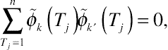
Alternatively, the statistical test on a polynomial time function can be performed by using the likelihood ratio test. For two successive linear mixed models specifying two different time functions, denoted by f⌢i−1 and f⌢i, respectively, the likelihood ratio test score is given by
where ˆβ(⌢i−1)1 and ˆβ(⌢i)1 are the estimated regression coefficients of the time polynomials obtained from the models with time functions f⌢i−1 and f⌢i, respectively, ˆβr is the vector of the estimated regression coefficients of other covariates, and Gβ1(⌢i−1,⌢i) is the likelihood ratio test statistic measuring whether the functional form f⌢i gains statistical information as compared to the functional form f⌢i−1. The statistic Gβ1(⌢i−1,⌢i) is asymptotically distributed as χ2 with one degree of freedom if the null hypothesis on the difference between ˆβ(⌢i−1)1 and ˆβ(⌢i)1 holds. Within the brace on the right of Equation (3.40), the first term is the log-likelihood ratio statistic for the model with polynomials f⌢i−1, whereas the second term is the same statistic for the model with the polynomial function f⌢i. If Gβ1(⌢i−1,⌢i)<χ2(1-α;1), the specification of f⌢i does not improve the model fit, thereby suggesting that f⌢i should be dropped from further comparison and the function f⌢i−1 should be retained. If Gβ1(⌢i−1,⌢i)>χ2(1−α;1), the specification of the polynomial function f⌢i predicts the pattern of change over time in Y statistically better than the functional form f⌢i−1, and accordingly, this functional form should be retained for further comparison and f⌢i−1 should be dropped. Eventually, the most appropriate time function can be determined statistically from those ⌢n functions ordered by complexity of the specified polynomials.
Sometimes, irregular time trends occur. For those irregular patterns of change over time, even the use of high-order polynomials cannot predict the time trend correctly. The situation can become more complex if different population groups display different patterns of change over time. Although the specification of multiple interaction terms can reflect group differences in the time trend, including too many interaction terms can make the estimation of parameters statistically unstable, particularly for small samples. Fortunately, longitudinal data can be modeled by constructing a predesigned residual variance–covariance matrix, in which the time factor is specified as a classification factor. In this approach, the time trend is predicted as a discrete process where all the patterns of change over time, regular or irregular, linear or nonlinear, can be displayed. In Chapter 5, linear regression models related to this approach will be described.
3.5. Empirical illustrations: application of two linear mixed models
In this section, two empirical examples are provided to illustrate the application of linear mixed models in longitudinal data analysis. The first example uses the data of the DHCC Acupuncture Treatment study, a randomized controlled clinical trial on the effectiveness of acupuncture treatment on PTSD. The second example is a longitudinal analysis on the AHEAD data, a large-scale national survey for older Americans. The purpose of including two examples is to illustrate the application of linear mixed models to analyze two different types of longitudinal data, one obtained from a clinical experimental study and one from a large-scale observational survey.
3.5.1. Linear mixed model on effectiveness of acupuncture treatment on PCL score
In (Section 2.2.4), an empirical example of a two-factor repeated measures ANOVA was presented on the pattern of change over time in the PCL score for two treatment groups, using the longitudinal data of the DHCC Acupuncture Treatment study. Given the limitations of the repeated measures ANOVA in longitudinal data analysis, in this section a linear mixed model is created for reanalyzing the data. Basic specifications of the time and the treatment factors are the same (TIME: 0 = baseline survey, 1 = 4-week follow-up, 2 = 8-week follow-up, 3 = 12-week follow-up; TREAT: 1 = receiving acupuncture treatment, 0 = else). The time factor in the model, however, is treated as a continuous variable, partitioned into three components – linear, quadratic, and cubit – for capturing the pattern of change over time in the PCL score. Furthermore, time is rescaled to be centered at point 1.5 for reducing multicollinearity in the three polynomial terms. The three time polynomials are denoted by CT, CT_2, and CT_3, respectively. The dependent variable, PCL_SUM, remains the same, as previously specified. As defined, TIME is a within-subject factor as it reflects intraindividual changes in the PCL score, while TREAT, on the other hand, is a between-subjects variable.
As PCL_SUM is a continuous variable measured at four time points, it is appropriate to apply a linear mixed model. The null hypotheses in this analysis are the same as previously specified in the repeated measures ANOVA. First, PCL_SUM is assumed to be constant over time in both the treatment groups; second, there is no interactive effect on PCL_SUM between TIME and TREAT; and third, there is no subject effect given the specification of two model covariates. The intercept, the effect of CT, and the effect of CT_2 are assumed to vary across subjects, and therefore, three random effects are specified. Correspondingly, the effects of CT_3 and TREAT are assumed to be fixed. Given the specification of the random effects for the intercept and for the regression coefficients of two covariates, this linear mixed model is a linear random coefficient model. The data structure for this analysis is of a block design (each subject supposedly has four observations), and therefore, the temporary dataset TP2, created in SAS Program 2.4, should be converted to a univariate data format. Below is the SAS code for this linear mixed model.
SAS Program 3.1:
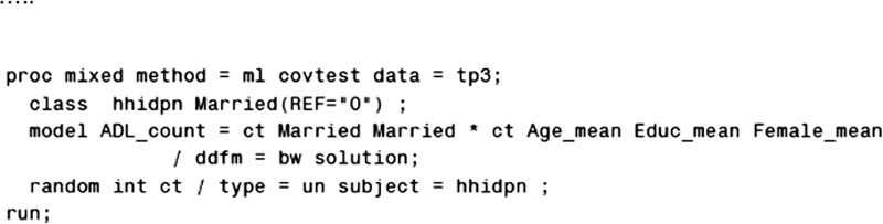
In SAS Program 3.1, the first DATA step creates a temporary univariate dataset, named TP3, converted from the temporary dataset TP2. Next, the centered time factor CT is constructed, based on which the quadratic and cubic centered time components, CT_2 and CT_3, respectively, are also created. A new temporary dataset, TP4, containing the three centered time polynomials, is then created. In the PROC MIXED procedure, I request SAS to estimate the regression coefficients of the covariates on PCL_SUM. In the PROC MIXED statement, the option METHOD = ML specifies the use of the maximum likelihood estimator for the estimation of the fixed effects. The CLASS statement specifies the subject ID and TREAT as classification factors. The TREAT(REF = “0”) option tells SAS to use “TREAT = 0” as the reference level; without this option, SAS designates “1” to be the reference as default. The MODEL statement specifies seven covariates: three time polynomials, TREAT, and the interaction terms between TREAT and each of the three time polynomials. The specification of the linear, quadratic, and cubic time components is based on the observed pattern of change over time in the raw data (see Chapter 2). The interaction terms are created because the time trend in the PCL score is observed to differ markedly between the two treatment groups. Also in the MODEL statement, the option “DDFM =” specifies the method for computing the denominator degrees of freedom in the F-test on the fixed effects. As the longitudinal data for this example came from a small sample, the Kenward and Roger method (1997) is used by specifying the DDFM = KR option. The option SOLUTION requests SAS to produce a solution for the fixed-effects parameters.
The RADOM statement specifies three random effects for the intercept, the linear component of centered time, and the quadratic term of centered time. The R matrix, containing residual variance, is not particularly specified in the PROC MIXED procedure as its specification is default in SAS. The TYPE = UN option tells SAS to estimate an unspecified covariance structure for the three random effects, and therefore, an unstructured (3 × 3) G matrix is produced. Additionally, the SUBJECT = ID option in the RANDOM statement specifies that the intercept of PCL_SUM and the slopes of CT and CT_2 for a given subject are independently distributed as those for others.
In both the MODEL and the RANDOM statements, some additional options can be specified for predicting the random effects for each subject, based on which subject-specific and group-averaged trajectories of the PCL score can be plotted and displayed. Given the focus of this chapter, the methods and applications for linear predictions will be discussed in Chapter 4, in which approximations of the random effects and predictions of the repeated measurements are the main focus.
SAS Program 3.1 yields a number of output tables. The Model Information table is not presented. Other than the basic information of data indicated above, the key information in that table is summarized as follows. In the analysis, the residual variance is profiled from optimization (the profile method for estimating the residual variance will be described in Chapter 4). The estimated method for the fixed effects is the maximum likelihood, denoted by ML. There are altogether 304 observations, with 189 being used in fitting the linear mixed model on the PCL_SUM repeated measurements. The −2 log-likelihood for this linear mixed model is 1399.6, statistically significant given a chi-square distribution on the null hypothesis. Other than the −2 log-likelihood statistic, some other more refined indicators of model fit are also produced from SAS Program 3.1, including AIC, AICC, and BIC (these additional model fit statistics will be introduced in Chapters 5 and 14). Values of the four fit statistics are very close, thereby generating the same conclusion about model fit for this analysis.
Next, I report the analytic results of the solution for the fixed effects and the Type 3 test results based on the F-statistic, given below.
SAS Program Output 3.1:
The Solution for Fixed Effects table displays the estimates for the fixed effects from the ML estimator. The intercept, 51.99 (se = 2.47), is the expected PCL score at the midpoint between the second and the third time points (time is centered at 1.5) for those in the control group (scaled zero). Among the three main effects of the time polynomial terms, the fixed effect of CT is 1.24, not statistically significant (t = 0.54, p = 0.59), and the regression coefficients of the quadratic and the cubic polynomials are −0.51 and −1.91, respectively, also statistically insignificant at α = 0.05 (for CT_2: t = −0.70, p = 0.49; for CT_3: t = −1.91, p = 0.08). The main effect of TREAT is −13.44, statistically significant (t = −3.74, p = 0.0005). Of the three interaction terms between TREAT and the three time components, the fixed effect for the interaction between TREAT and CT_2 is statistically significant (t = 4.97, p < 0.0001), whereas those for the other two terms are not. Given the statistical criterion that the main effects of two independent variables should be regarded as statistically meaningful if the interaction between them is statistically significant, the fixed effects of all three time components are considered statistically significant in this analysis. The Type 3 tests for the fixed effects yield the summary results on the statistical significance of the regression coefficients, supporting the conclusions concerning the fixed effects.
The fixed effects of the three time polynomials, TREAT, and the interaction terms take inconsistent signs. Given the complex combinations of the fixed effects, it is difficult to generalize a pattern of change over time in the PCL score directly from the fixed effects. Therefore, the random effects need to be approximated for each subject and then used to predict the PCL score both individually and for each of the two treatment groups. By plotting those predictions, the pattern of change over time in the PCL score and its differences between the two treatment groups can be displayed and analyzed. Therefore, additional procedures are required to complete this analysis, as will be presented in Chapter 4.
The RANDOM statement in SAS Program 3.1 also produces an output for the estimates of the unstructured variance and covariance components. Given the focus of this chapter on the estimation of the fixed effects, the results of the random components will be illustrated and discussed in Chapter 4.
3.5.2. Linear mixed model on marital status and disability severity in older Americans
In the second example, I illustrate the application of a linear mixed model on the longitudinal data of the AHEAD survey (the information about the survey was described in Chapter 1). In the analysis, I use data from the six waves starting with the 1998 wave (1998, 2000, 2002, 2004, 2006, and 2008). Given the illustrative nature, the AHEAD selected sample, including 2000 subjects, is used. The selected sample is named AHEADALL_2000.
In this illustration, I propose to analyze the effect of a person’s marital status on disability severity among older Americans. The disability severity score is defined as health-related difficulty in performing activities of daily living (ADL), consisting of five task items (dress, bath/shower, eat, walk across time, get in/out of bed). For each item, measured at six time points, disability is scored one if the person has difficulty, personal help, or equipment help for health-related reasons and scored zero if otherwise. The ADL count is used as the outcome variable, named ADL_COUNT in the analysis, with its value ranging from 0 to 5 at each time point (Verbrugge and Liu, 2014). Marital status, used as the main independent variable or, as I call it, the index predictor, is a dichotomous variable, named MARRIED in the analysis, with 1 = currently married and 0 = else. As marital status is measured at each of the six time points, MARRIED is a time-varying covariate.
The AHEAD data come from a large-scale observational survey, so that there is no randomization performed in data collection. Therefore, the bivariate association between marital status and disability severity can be confounded by the influence of some lurking covariates. Given this concern, three potential confounders are identified: age, educational attainment, and gender. These three variables are considered the controls because each of them is observed to be causally associated with both marital status and disability, thus may potentially yield confounding effects. An individual’s age is the actual years of age and educational attainment is an approximate proxy for socioeconomic status, measured as the total number of years in school, assuming the influence of education on an older person’s health to be a continuous process (Liu et al., 1998). Gender is a dichotomous variable: 1 = women and 0 = men. These three variables are measured at the AHEAD baseline survey, and for analytic convenience, they are rescaled to be centered at the sample means, termed Age_mean, Educ_mean, and Female_mean, respectively. Empirically, the mean of a dichotomous variable indicates the likelihood or propensity of being in the group coded 1; in the present analysis, the variable Female_mean can be understood as the expected proportion of the population the sample represents who are women. In multivariate regression analysis, centering a dichotomous variable is valid only when it is used as a confounder. If a dichotomous variable is specified as the index predictor, it is inappropriate to center it because prediction of the outcome at its mean corresponds to a nonexistent stratum (Muller and MacLehose, 2014).
In this illustration, the primary goal is to examine whether the ADL count differs significantly between those currently married and those currently not married after adjusting for the confounding effects of age, educational attainment, and gender. As the ADL count is a continuous variable measured at six time points, a linear mixed model is created on repeated measurements of the ADL count. Two null hypotheses are advanced for the analysis: the ADL count does not change over time, and the ADL count does not differ between those currently married and those currently not married, other variables being equal. Given the results of a preliminary data analysis, only the linear term of time needs to be specified in the linear mixed model. That is, the ADL count is found to be linearly associated with time. Correspondingly, the linear mixed model specifies two random effects for the intercept and for the slope of CT, whereas the effects of marital status, the interaction between marital status and time, and the three control variables are assumed to be fixed across subjects. Given the specification of two random effects, the mixed model is also a linear random coefficient model.
Given the focus of this chapter on the estimation of the fixed effects, for the time being the primary concern is in the estimated regression coefficients of covariates. The pattern of change over time in the ADL count and its differences between the two marital status groups will be illustrated in the succeeding two chapters. Below is the SAS program for the current step.
SAS Program 3.2a:
In SAS Program 3.2a, the first DATA step creates a temporary univariate longitudinal dataset, TP1, from the original multivariate dataset AHEADALL.2000, together with the construction of the time-varying response variable ADL_COUNT. The second data step creates a temporary dataset, TP2, containing centered time variable CT, the time-varying index predictor married, and the three centered control variables. Next, the third temporary dataset, TP3, is constructed for the application of the linear mixed model on the ADL count. The SAS program for the model is presented below.
SAS Program 3.2b:
The basic syntax of SAS Program 3.2b is analogous to that of SAS Program 3.1. Given the large sample size for the analysis, the between-within method is used to compute the denominator degrees of freedom in the F-test on the fixed effects, so that the DDFM = BW option is specified in the MODEL statement.
The above program yields a number of output tables on the model fit information and the fixed effects. According to the output tables displaying the model information and the model fit statistics, not presented, the temporary dataset, TP3, is the data used in the analysis, and the dependent variable is designated as ADL_COUNT. The covariance structure is still UN, with HHIDPN, the subject identification number used in the AHEAD data, being the unit for the subject effect. The residual variance is again profiled from optimization. The estimating method for the fixed effects is ML. There are altogether 12,000 observations at six time points with a selected sample of 2,000 subjects, with 6,555 observations used in fitting the linear mixed model on the ADL count. The −2 log-likelihood for this linear mixed model is 19,897.3, corresponding to a large sample size. The model fit statistics from the other three methods, AIC, AICC, and BIC, are all close to the −2 log-likelihood statistic, leading to the same conclusion concerning the goodness-of-fit.
The solution for the fixed effects and the Type 3 test results are presented in the following output tables.
SAS Program Output 3.2:
The fixed effects, as generated from the maximum likelihood estimator, are presented in the Solution for Fixed Effects table. All the fixed effects are statistically significant with p-values smaller than 0.0001. The intercept, 1.33 (se = 0.04), is the expected ADL count at the midpoint between the third and the fourth time points (time is centered at 3.5) among those currently not married, other covariates being equal on average conditions. The fixed effect of time is positive (0.13), indicating that the ADL count among those currently not married is expected to increase by 0.13 with a 2-year increase in time, other variables being equal. The main effect of married is −0.21 and the interaction between marital and time is also negative (−0.04), both statistically significant, which, combined, suggest a lower ADL count among those currently married than among those currently not married. The negative effect of marital status tends to get stronger over time given the negative sign of the interaction. With respect to the three control variables, age is positively associated with ADL_COUNT (βage = 0.06, p < 0.0001), educational attainment is negatively linked to the disability severity (βedu = −0.06, p < 0.0001), and older women are expected to have an ADL count 0.29 points higher than older men (βfemale = 0.06, p < 0.01), other covariates being equal. The Type 3 tests confirm the strong statistical significance for all the fixed effects.
Like the first example, the random effects for each subject need to be predicted and then used to derive the ADL count predictions for displaying the trajectory in the ADL count and its group differences. The methods for linear predictions will be described in Chapter 4, with the illustration based on the same linear mixed model.
3.6. Summary
As the entire body of linear mixed models includes a large number of complex procedures for inferences, estimations, optimizations, and approximations, this chapter is focused on the description of statistical procedures on the estimation of the fixed effects. I start the chapter with three simple cases in the construct of linear mixed models to lead the reader into the realm of mixed-effects modeling. Based on the three cases, linear mixed models are formalized by using matrix algebra, which is followed by statistical inferences on the fixed effects and the delineation of various time trend patterns. In Section 3.5, two empirical examples are provided for illustrating the application of linear mixed models in longitudinal data analysis.
As widely applied in the estimation of model parameters in other types of regression models, the maximum likelihood approach is a popular estimator to derive the fixed effects in linear mixed models. When the sample size is small, however, the maximum likelihood estimator yields a variance estimate that is biased downward because a penalty term is missed given unknown population means. This issue can be resolved by applying the REML estimator, an empirical Bayes estimator that corrects the downward bias in MLE, as will be described in the next chapter. Given the widespread applications of Bayes-type techniques in longitudinal data analysis, I will start Chapter 4 with a section providing a brief introduction of the basic Bayes theory and Bayesian inference before proceeding with the description of the REML estimator.

 (3.3)
(3.3)

 (3.5)
(3.5) (3.7)
(3.7) (3.8)
(3.8)


 (3.12)
 (3.13)
 (3.14)
 (3.15)
 (3.16)
 (3.17a)
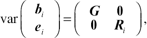 (3.17b)
 (3.20)
 (3.21)
 (3.22)
 (3.23)
 (3.24)
 (3.25)
 (3.26)
 , where β0 is the population parameter vector, tends to converge in probability to a normal vector with mean 0 and the covariance matrix
 corresponding to βm, given by
 (3.27)
 (3.28)
 (3.29)
 (3.30)
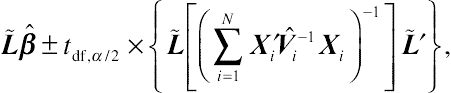 (3.31)
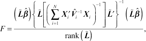 (3.32)