
12.4. Empirical illustration: predicted transition probabilities in functional status and marital status among older Americans
In this illustration, I analyze longitudinal transitions in functional status among older Americans and their differences between those currently married and those currently not married, with the use of the AHEAD longitudinal data. Mortality is used as a competing health state to handle selection bias in health transitions. Accordingly, six types of transitions are specified from two origin states, functional independence and functional dependence (denoted as origins 0 and 1), to three destination states, functional independence, functional dependence, and deceased between two successive waves (denoted by destinations 3, 1, and 2). The reason to reverse scores of the destination states will be explained below.
12.4.1. Measures, models, and SAS programs
With the specification of six data points, the six types of transitions in functional status are analyzed for the following five time intervals: (1) from T0 (1998) to T1 (2000), (2) from T1 (2000) to T2 (2002), (3) from T2 (2002) to T3 (2004), (4) from T3 (2004) to T4 (2006), and (5) from T4 (2006) to T5 (2008). For each time interval, the probability for experiencing a given type of transition is denoted by  , where
  and k refer to the origin and the destination states, respectively.
Given the structure of the outcome data, the mixed-effects multinomial logit transition model, described above, is applied to predict the six transition probabilities in each of the five time intervals. As specified, the origin state  is a covariate. Operationally, the dichotomous variable ADL_BIN at time point j − 1, taking value 0 or 1 and defined previously, is used to measure the origin state . As a covariate in this analysis, ADL_BIN is renamed ADL_BAS. The outcome variable in the mixed-effects multinomial logit transition model is named HEALTH_DES, defined as HEALTH_DES = 3 (functional independence), HEALTH_DES = 1 (functional dependence), and HEALTH_DES = 2 (dead in a given time interval), respectively. Following the tradition in SAS programming, HEALTH_DES = 3 is used as the reference level. Marital status is the previously defined dichotomous variable, with 1 = currently married and 0 = currently not married, but is measured at time point j − 1 rather than at j. The three centered covariates, AGE_MEAN, EDUC_MEAN, and FEMALE_MEAN, continue to be used as the controls. According to the results of a preliminary analysis, an interaction term between time and ADL_BAS is specified to capture the possible convergence of the effects of the origin state. Some other interactions, such as TIME × MARRIED and ADL_BAS × MARRIED, were also considered and tested, but their inclusion was not found to contribute significantly to the model fit and thus was removed.
The random intercept multinomial logit regression is applied again for computational simplicity. The SAS PROC NLMIXED procedure is applied to compute both the fixed and the random effects for the random intercept multinomial logit transition model, with adaptive Gaussian quadrature being used to approximate the integral of the likelihood over the random effects. Given the specification of the random intercepts, the variable TIME is treated as a continuous variable. The full random intercept multinomial logit model, defined in Chapter 11, is selected as the basic perspective for estimating model parameters with its relatively high predictive power. After the analytic results are generated from the full model, the retransformation method is applied for nonlinear predictions of the transition probabilities, including retransformation of both the between-subjects and the within-subject random components. For comparative purposes, the predicted transition probabilities from the empirical BLUP are also computed and displayed. The delta method is applied to compute the variances of the predicted probabilities.
The retransformation method is based on a series of mean multinomial logit functions with the covariates rescaled to be centered at purposefully selected values. As a result, it is unrealistic to present the entire set of procedures for computing the transition probabilities and the differences in such nonlinear predictions between the two marital status groups. Therefore, in this illustration, I only display the computational steps for the third time interval, from T2 (2002) to T3 (2004). From this presentation, the reader can learn how to compute the transition probabilities for other time intervals. Correspondingly, the time variable should be rescaled to be centered at the fourth time (TIME = 6), thereby resulting in the specification “t = TIME − 6.” From the same rationale, covariates ADL_BAS and MARRIED, both 0–1 dichotomous variables, should be measured at the third time point. Therefore, when MARRIED and ADL_BAS are scaled zero and the three control variables are centered at sample means, the intercepts predict the mean logits for transitions from functional independence to the three destination states among those currently not married and between the third (TIME = 4) and the fourth time (TIME = 6).
As indicated in the previous two chapters, the application of the PROC NLMIXED procedure requires the robust starting values of the specified parameters. Therefore, the PROC GLIMMIX procedure is applied first to yield an initial set of parameter estimates, which are then borrowed as the robust starting values of both the fixed and the random effects for the execution of the PROC NLMIXED procedure. The following SAS program specifies this GLIMMIX model.
SAS Program 12.1a:

In SAS Program 12.1, the specification of the time factor starts with one (time 0 is the first baseline time for measuring the covariate ADL_BAS). Also in the DATA TP1 step, the variables ADL_DES and DEATH are specified as the destination states for each time interval, and therefore, they are measured at the current time point. In contrast, the variable ADL_BAS, indicating the functional status of origin, is measured at the prior time point. In the temporary dataset TP2, time is rescaled to be centered at the fourth time, and the variable MARRIED is measured at the prior time point. Given the creation of these variables for the analysis of transitions in functional status, the random intercept multinomial logit transition model can be constructed by using the PROC GLIMMIXED procedure, as displayed in the following SAS program.
SAS Program 12.1b:
……
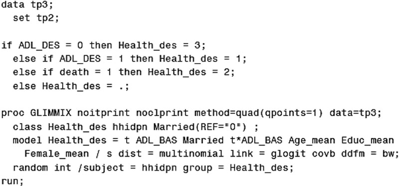
In SAS Program 12.1b, the destination state variable HEALTH_DES is created first according to the aforementioned definition (1 = functional dependence, 2 = dead between two successive waves, and 3 = functional independence). The model part is mostly the same as SAS Program 11.1. Of the modifications, the variable ADL_BAS is now specified as a covariate and MARRIED is included in the CLASS statement with those currently not married serving as the reference group. With the origin state variable ADL_BAS included on the right of the MODEL statement, HEALTH_DES indicates the multidimensional outcomes of transitions in the third time interval given the value of ADL_BAS. The other attached options in the GLIMMIX procedure are interpreted in Chapter 11.
With the parameter estimates from the above PROC GLIMMIX procedure, not presented, the starting values of the parameters can be specified in the PROC NLMIXED procedure, as presented below.
SAS Program 12.2
……:

SAS Program 12.1 is analogous to SAS Program 11.2, with the exception of a different set of starting values, the addition of ADL_BAS in the covariates, and the specification of the PREDICT statements to derive the empirical BLUPs. The SAS code for creating the scoring dataset, used to compute the empirical BLUPs, is not displayed given its similarity to the syntax presented in Chapter 11. The PROC MEANS procedure is called to derive the empirical BLUPs of the transition probabilities.
12.4.2. Prediction of transition probabilities
SAS Program 12.2 generates the analytic results of the random intercept multinomial logit transition model with time being centered at six (the fourth time point), ADL_BAS and MARRIED being measured at four (the prior time point), and the three controls being centered at sample means. The following output tables present the main portion of the analytic results that are required to predict the transition probabilities in functional status in the third time interval for those currently not married.
SAS Program Output 12.1a:

It was indicated previously that all the regression coefficients of a given covariate on the multinomial logit components should be regarded as statistically meaningful if any of them is statistically significant. Given this criterion, the regression coefficients in the first output table are all statistically significant. Both the random intercept terms, given the same criterion, are also regarded as statistically significant. The parameter estimates of the within-subject random terms for the intercepts, obtained from the variance–covariance matrix for the multinomial logits, are displayed in the second output table. These analytic results, however, are difficult to interpret before being translated into the transition probabilities and the conditional effects. Below, a step-by-step presentation is provided to display how to convert the above analytic results into the transition probabilities.
In this random intercept multinomial logit transition model, time is centered at 6, ADL_BAS and MARRIED are the original 0–1 dummy scores at the third time (TIME = 4), and the three control variables are centered at sample means. Consequently, the intercept estimates predict the marginal means of the multinomial logits for transitions in the third time interval from functional independence (ADL_BAS = 0) to the three health outcomes – functional independence, functional dependence, and dead – for those currently not married (MARRIED = 0). Therefore, only the fixed and the random estimates for the intercepts need to be accounted for in computing the three transition probabilities for those currently not married in the third time interval (TI = 3). Correspondingly, the S11 and S22 estimates plus the subset of the intercepts in the variance–covariance matrix for the fixed effects can be used as the approximate variance–covariance matrix for the marginal means of the multinomial logits. With these estimates, the next step is to calculate the transition probabilities from functional independence to functional dependence and death for those currently not married in the third time interval. The following is the detailed computation.


where  is the predicted transition probability from functional independence to functional dependence in the third time interval (between the third and the fourth time points) for those currently not married (represented by superscript N). Similarly,
  is the death rate between the third and the fourth time points among those currently not married who are functionally independent at the third time point (TIME = 4). By definition,
  , the transition probability from functional independence to functional independence in the third time period for those currently not married, is the residual to the sum of the two nonreference transition probabilities, written as
  .
.
By borrowing Equations (11.28) and (11.29), the 2 × 2 variance–covariance matrix can be created for the two nonreference transition probabilities for those currently not married. First, by using the analytic results presented in SAS Program Output 12.1a and Equation (11.28), the four elements in the B matrix are  ,
,  , and
, and  , respectively. Given the approximated variance– covariance matrix for the predicted multinomial logits, the variance–covariance matrix for the predicted transition probabilities
  and
and  at the third time interval (TP = 3) for those not married at the third time point can be approximated by the use of Equation (11.29), given by
where  denotes the variance–covariance matrix for the two transition probabilities. The diagonal elements in the final matrix yield the variance approximates of the two predicted transition probabilities in the third time interval among those not married at the third time point, written as
  and
and  , respectively. The square root of each variance approximate yields the corresponding standard error estimate, given by
  and
and  , respectively.
SAS Program 12.2 also derives the empirical BLUPs for the three transition probabilities by the creation of a scoring dataset and the use of the PROC MEANS procedure. The results are presented in the following SAS output table.
SAS Program Output 12.1b:

Clearly, for those not married at the third time point, the empirical BLUP approach yields close nonlinear predictions of the transition probabilities to those from the retransformation method. The empirical BLUP standard errors, noted as the standard deviation in the above output table, are severely underestimated due to the neglect of a portion of the random components in the retransformation process.
The computation for the transition probabilities for those currently married can be performed in the same fashion. First, a random intercept multinomial logit transition model is created by replacing the variable MARRIED with its reversed version UNMARRIED, specified as 0 = currently married and 1 = currently not married. The SAS program for this model is exactly the same as SAS Program 12.2 except for minor modifications. In addition to the use of UNMARRIED in the covariates, the starting values of the regression coefficients for this reversed variable need to take the opposite signs as those specified in SAS Program 12.2. Furthermore, in creating the scoring dataset for those married at the third time point, the option MARRIED = 0 should be replaced with MARRIED = 1. In multivariate regression modeling, a change in the order of the 0–1 score for a dichotomous variable does not affect the estimation of parameters and the model fit, and the only changes in the analytic results are the values of the intercepts and the reversion of the sign for the regression coefficient of the dichotomous independent variable.
Given its tremendous resemblance to SAS Program 12.2, the SAS program for those married at the third time point is not displayed. The modified SAS program produces the following analytic results.
SAS Program Output 12.2a:

According to the statistical criterion indicated earlier, all the regression coefficients and the random effects in the first output table are statistically significant. With time being centered at six, ADL_BAS and UNMARRIED are each scaled at zero, and the three control variables are centered at sample means; the intercept estimates predict the marginal means of the multinomial logits for the transitions in the third time interval from functional independence (ADL_BAS = 0) to the three destination states at the fourth time point for those married at the third time point (UNMARRIED = 0). As a result, the three transition probabilities for those married at the third time point (TIME = 4) can be readily computed by using the fixed and the random effects for the intercepts only. Given the analytic results displayed above, the first two transition probabilities in the third time interval for those currently married are computed as


where  is the predicted transition probability from functional independence to functional dependence in the third time interval (between the third and the fourth time points) for those married at the third time point (denoted by superscript M), and
  is the death rate between the third and the fourth time points among those married and functionally independent at the third time point. The transition probability from functional independence to functional independence in the third time interval for those married at the third time point, denoted by
  , is the residual to the sum of the two nonreference transition probabilities, written as
  .
.
Using Equations (11.28) and (11.29) again, a 2 × 2 variance–covariance matrix is computed for the two nonreference transition probabilities for those married at the third time point. The four elements in the B matrix are exactly the same as those for the currently not married, namely, , , and . With these approximates, the variance–covariance matrix for the predicted transition probabilities at the third time period (TP = 3) for those currently married, denoted by  , is approximated by

Therefore, the variance approximates for the two predicted transition probabilities for the third time period among those married at the third time point are 0.008 and 0.0002, respectively, very close to those for their unmarried counterparts. Likewise, the standard error approximates of the two predicted transition probabilities are 0.088 and 0.015, respectively. The empirical BLUPs for the three transition probabilities in the third time interval for those currently married are shown below.
SAS Program Output 12.2b:

As presented, for those who are married at the third time point, the empirical BLUPs are close to nonlinear predictions of the transition probabilities from the retransformation method; the empirical BLUP standard errors, however, are severely underestimated.
With regard to transitions from functional dependence to the three destination health states, the transition probabilities and the associated variance–covariance matrix can be computed by applying the same procedure. In this computation, the scale of the variable ADL_BAS needs to be reversed, with 1 = functional independence and 0 = functional dependence at the beginning of a given time interval, named ADL_BAS1 in the analysis. Consequently, when time is centered at the end point of the time interval, the variable MARRIED is scaled zero, and the three control variables are centered at sample means; the intercepts represent the marginal means of the multinomial logit components for transitions from functional dependence to the three destination states for those not married at the beginning of the time interval. As indicated earlier, in multivariate regression modeling, reversing the scale of a dichotomous covariate does not affect the estimation and model fit at all.
With a series of tedious computations, a complete set of transition probabilities and the associated standard errors can be predicted from the results of the random intercept multinomial logit transition model. Table 12.1 displays nonlinear predictions of the transition probabilities in five time intervals and among those married and not married at the beginning of each interval. The standard error approximates for the nonreference transition probabilities are presented in parentheses.
Table 12.1
Transition Probabilities From Two Origin States to Three Destination States in Five Time Intervals: Older Americans (N = 2000)
| Transition Type | Time Interval | ||||
| T0–T1 | T1–T2 | T2–T3 | T3–T4 | T4–T5 | |
| For Those Currently Not Married | |||||
|
|
0.172 (0.090) | 0.172 (0.088) | 0.170 (0.088) | 0.170 (0.088) | 0.171 (0.089) |
|
|
0.091 (0.014) | 0.094 (0.014) | 0.092 (0.014) | 0.092 (0.015) | 0.093 (0.015) |
|
|
0.737 | 0.735 | 0.738 | 0.738 | 0.737 |
|
|
0.187 (0.103) | 0.190 (0.106) | 0.195 (0.110) | 0.194 (0.110) | 0.195 (0.112) |
|
|
0.098 (0.025) | 0.098 (0.025) | 0.099 (0.026) | 0.098 (0.110) | 0.099 (0.112) |
|
|
0.715 | 0.712 | 0.706 | 0.708 | 0.706 |
| For Those Currently Married | |||||
|
|
0.170 (0.088) | 0.170 (0.088) | 0.170 (0.088) | 0.171 (0.088) | 0.171 (0.089) |
|
|
0.092 (0.015) | 0.092 (0.014) | 0.092 (0.015) | 0.092 (0.016) | 0.093 (0.018) |
|
|
0.738 | 0.738 | 0.738 | 0.737 | 0.736 |
|
|
0.186 (0.102) | 0.189 (0.106) | 0.198 (0.113) | 0.193 (0.110) | 0.195 (0.112) |
|
|
0.098 (0.024) | 0.098 (0.025) | 0.100 (0.028) | 0.098 (0.110) | 0.099 (0.112) |
|
|
0.716 | 0.713 | 0.703 | 0.708 | 0.706 |

Notes: ![]() , transition probability from independence to dependence (incidence);
, transition probability from independence to dependence (incidence); ![]() , death rate in time interval for those functionally independent at the beginning of interval;
, death rate in time interval for those functionally independent at the beginning of interval; ![]() , transition probability from independence to independence (persistence);
, transition probability from independence to independence (persistence); ![]() , transition probability from dependence to dependence (persistence);
, transition probability from dependence to dependence (persistence); ![]() , death rate in time interval for those functionally dependent at the beginning of interval;
, death rate in time interval for those functionally dependent at the beginning of interval; ![]() , transition probability from dependence to independence (recovery). As the residual probabilities to their nonreference counterparts,
, transition probability from dependence to independence (recovery). As the residual probabilities to their nonreference counterparts, ![]() and
and ![]() do not have the predicted standard error estimates.
do not have the predicted standard error estimates.
The predicted transition probabilities shown in Table 12.1 do not necessarily agree with those from the sample margins. The predictions presented in this table are all normalized to sample means of the observed and unobserved control factors in the application of the random intercept multinomial logit transition model, while the sample margins can be massively confounded by population heterogeneity. Furthermore, the derivation of these model-based transition probabilities is based on the assumption that only one transition be permitted within a given time interval. This one-step transition hypothesis is reasonable for older persons, particularly for those aged over 85 years, among whom resolution from the loss of functional ability generally takes a long-term process (Liu et al., 1995).
As displayed in Table 12.1, the incidence rate of disability during a 2-year time interval is about 0.17, and this rate is constant throughout all five time intervals. Also, this incidence rate is similar between those not married and those married at the beginning of a time interval. This incidence result indicates that among those functionally independent at a prior time point, married or not, about 17% are expected to become functionally dependent at the end of a time interval, other variables being equal. The death rate during each time interval is also fairly stable over time. While the death rates for those married and those not married are very close, the older persons functionally dependent at the beginning of each time interval are associated with a slightly higher mortality than those functionally independent. Among those functionally independent at the beginning of the time interval, the majority stay functionally independent within a time interval, with the proportion being around 0.74. Such a persistence rate is consistent not only between those married and those not married but also over time. In contrast, of those functionally dependent at the beginning of each time interval, about 20% survive and remain disabled at the end of the interval. Notably, the interval-specific rate of resolution from functional dependence is as high as 0.71–0.72, suggesting that about 70% of those functionally dependent at the beginning of a given time interval are expected to recover from disability within a 2-year period, other covariates being equal. This high rate of resolution is probably due to the use of the ADL count as the measurement of disability, and using a more valid measurement in this health indicator may significantly lower this transition probability. This issue, however, is currently not of concern given the focus of illustrating a statistical technique.
The results reported in Table 12.1 provide strong evidence that in the mixed-effects multinomial logit transition model, statistically significant fixed effects of covariates on the logit scale do not necessarily translate into statistically significant effects on the probability scale. Even a sizable face value of the logit effect does not necessarily translate into a notable difference in the transition probability between two associated population subgroups. In conversion from the multinomial logit function to the transition probabilities, complex functional and effect retransformations are involved. Consequently, the size, dispersion, and even the sign of the logit coefficients can be altered after they are retransformed to the conditional effects on the transition probabilities. Considerable caution must be applied when attempting to interpret the analytic results of the mixed-effects multinomial logit transition model without further computations.
It must also be noted that the transition probabilities displayed above are population-averaged, not individual-based, reflecting the pattern of change over time in functional status transitions among surviving members. At different time points, samples of older survivors may have different distributions of individual health characteristics because those who are less fit are more likely to exit from further observation. Therefore, the transition patterns at the population level and at the individual level can differ markedly (Christensen et al., 2008). As discussed in Chapter 7, the survival of the fittest process can alter the population health composition continuously over time, especially among the oldest old. When such a structural change in population health composition exerts a strong effect, thereby masking the impact of individual aging on the time trend in health, the population-averaged health transitions will display a lack of distinctive patterns of change over time. In this process, tremendous population heterogeneity is disguised. For the analysis of individual-based patterns of change over time in health transitions, more refined methods need to be applied. This issue will be further discussed in the Section 12.5.
The results of predictions from the empirical BLUP are not displayed in Table 12.1. To summarize, in all the time intervals, the empirical BLUPs of the transition probabilities are close to those from the transformation method, but the standard errors are much underestimated. With the similarity of the BLUP results to those shown in SAS Program Outputs 12.1b and 12.2b, the BLUP predictions are not further presented.
12.4.3. Effects of marital status on transition probabilities
Table 12.1 displays that for each time interval, the predicted transition probabilities are highly consistent between those currently married and those currently not married. Yet, to display how to compute and evaluate the effects of a covariate on the transition probabilities, below I present an example of computing the conditional effects of marital status on the transition probabilities from functional independence to the three destination states. The third time interval is selected again for this illustration. Given Equation (11.25), the conditional effects of marital status on the three transition probabilities in the third time interval are given by
where  is the conditional effect of marital status on the predicted transition probability from functional independence to functional dependence in the third time interval, and
  is the corresponding conditional effect on mortality.
The statistical significance of the conditional effects of marital status on the two nonreference transition probabilities can be tested by Equation (11.27). The following computational steps derive the Wald chi-square statistics on the aforementioned conditional effects of marital status.

The Wald statistic is distributed asymptotically as a chi-square with one degree of freedom under the null hypothesis. Consequently, both the Wald chi-square statistics shown above are not statistically significant given α = 0.05. The evaluation of  , the residual effect of marital status, depends on the test results for the two nonreference effects, and therefore, all the three conditional effects of marital status in the third time interval are considered statistically insignificant.
Using the same computational procedure, the effects of marital status and the associated dispersion statistics for the other time intervals can be computed. Table 12.2 displays the complete set of the conditional effects of marital status on the transition probabilities from the two origin states to the three destination states for all five time intervals. The Wald statistics for the effects of marital status on the nonreference transition probabilities are presented in parentheses.
Table 12.2
Effects of Marital Status on Transition Probabilities From Two Origin States to Three Destination States: Older Americans (N = 2000)
| Time Interval | |||||
| Transition Type | T0–T1 | T1–T2 | T2–T3 | T3–T4 | T4–T5 |
|
|
−0.0019(1.5696) | −0.0014(9.1709) | 0.0002(0.6160) | 0.0003(0.4029) | 0.0003(0.2276) |
|
|
−0.0008(0.9740) | −0.0016(>100.0000) | 0.0002(0.0886) | 0.0003(0.0882) | <0.0001(0.0153) |
|
|
0.0011 | 0.0031 | −0.0004 | −0.0005 | −0.0003 |
|
|
−0.0007(1.1880) | −0.0005(11.3551) | 0.0029(1.0654) | −0.0007(16.8401) | −0.0004(5.2971) |
|
|
−0.0004(0.6402) | −0.0003(0.0433) | 0.0007(0.1704) | <−0.0001(0.0058) | <−0.0001(0.0063) |
|
|
0.0011 | 0.0007 | −0.0036 | 0.0007 | 0.0004 |

Note: The effects of marital status on the transition probabilities to functional independence depend on the testing results of the effects on the probabilities of the nonreference outcome states.
In Table 12.2,  ,
,  , and
, and  are the conditional effects of marital status on the transition probabilities from functional dependence to the three destination states, respectively. The other three indices, , , and , were specified previously. As expected, all the effects of marital status take very small values. Although some effects are statistically significant, their trivial face values do not translate into any substantively meaningful influences and thus should be ignored. With such insignificant effects, the current presentation is aimed at displaying the computational steps for predicting transition probabilities and the group differences in the predictions.
It may be indicated that the aforementioned procedure can be applied to generate age-specific transition probabilities in aging and health research. Therefore, the approach can be well adapted into an algorithm for constructing an active life table, both periodic and cohort-specific. The standard errors of the transition probabilities and other life table measurements can be easily approximated by applying the multidimensional and multivariate modeling technique.
12.5. Summary
In this chapter, a new approach is delineated and empirically illustrated for the analysis of longitudinal transitions from two or more states of origin to a set of destination states. Technically, the method is just an extension of the mixed-effects multinomial logit model described in Chapter 11, with the use of the response at the prior time point as a covariate. Linking to a specific value of the prior state, nonlinear predictions of a set of the response probabilities can be interpreted as the transition probabilities from a given origin state to a set of destination states. With the inclusion of theoretically relevant predictor variables and the specified random effects, intraindividual correlation in longitudinal transition history is adequately accounted for. Knowing the expected values of both the observed and the unobserved explanatory factors, the marginal means of a set of transition probabilities can be predicted, with their dispersions statistically approximated. Although computationally tedious, this multidimensional transition model can be conducted speedily by appropriate computer programming.
The statistical approach introduced in this chapter can be well extended to generate age-specific transition probabilities, thereby enabling the construction of an active life table in aging and health research. For example, with a longitudinal design of 2-year intervals, age can be categorized into a series of 2-year age groups. It follows then that in the resulting matrix of the transition probabilities from the mixed-effects multinomial logit transition model, the diagonal elements approximate the cohort-specific transition probabilities, whereas the vertical elements can be regarded as period-specific transition probabilities for a synthetic birth cohort. While the classical active life table approaches have been criticized for their lack of capability in accounting for the impact of population heterogeneity, the mixed-effects multinomial logit transition model offers a sound statistical perspective, in which many statistical and specification problems in longitudinal data analysis can be appropriately handled.
It is contended that the mixed-effects binary logit model can derive equally robust, consistent results in the analysis of health transitions. Strictly speaking, such an approach should not be recommended for use. With the constraint that a set of transition probabilities must sum up to unity, nonlinear predictions of the transition probabilities are correlated, although the destination states are specified as mutually independent. An increase in one of the probabilities must be accompanied by a decrease in at least one of the others. Therefore, the covariance structure for a set of nonlinear predictions is multivariate, not univariate. The application of the mixed-effects multinomial logit transition model does not just provide a more efficient, consistent predictor for generating transition probabilities. While statistically resulting in better parameter estimates as compared to the binary perspective, the multinomial logit model also yields more valid and reliable dispersion statistics for the predicted transition probabilities. The variance–covariance matrix for the logit components, obtainable from the multinomial logit regression, can be retransformed to an approximate variance–covariance matrix for the transition probabilities. The approach for applying separate binary logit models may arguably generate unbiased nonlinear predictions of the transition probabilities; it does not, however, possess the statistical capability to handle the multivariate covariance structure in a set of transition probabilities. Therefore, this approach results in biased standard error estimates for the predicted transition probabilities.
The reader might want to bear in mind that the method illustrated in this chapter is focused on the derivation of the marginal means for a set of transition probabilities. Such transition probabilities are population-averaged, not individual-based, and in the longitudinal setting, they display the pattern of change over time in health status among survivors. For older persons, longitudinal trajectories of the transition probabilities are based on a series of follow-up samples selected by values of the dependent health variable. Therefore, any inference from the population-averaged time trend to the individual-based growth trajectory can yield incorrect conclusions. Individually, as an older person ages, the incidence rate of disability rises, recovery from functional limitations slows down, and mortality enhances. For a population, the strongest persons survive during a period of time, and the survivors are less likely to be functionally disabled than those who have been deceased. Consequently, the older population tends to be composed of physically and mentally selected individuals along the longitudinal course. Such a change in the population health composition massively offsets the effect of individual aging, thereby masking tremendous population heterogeneity inherent in health transitions. Pattern-mixture multinomial logit modeling, which is beyond the scope of this book, may be applied to generate pattern-specific transition probabilities in older persons.
..................Content has been hidden....................
You can't read the all page of ebook, please click here login for view all page.