
Residual and influence diagnostics
Abstract
In Chapter 6, the statistical methods of residual diagnostics are described first. A variety of residual types are specified, both generally and with specific regard to longitudinal data analysis. I also delineate semi-variogram, a popular residual diagnostic technique applied in longitudinal data analysis. This unique method is used to check whether serial correlation among repeated measurements for the same subject is present given the specified fixed effects and the covariance parameters. The method can be specified in both the random intercept and the random coefficient perspectives. Next, the statistical methods on influence diagnostics are displayed. The variety of the basic diagnostics to identify influential observations include the Cook’s distance statistic, leverage, the DFFITS score, the MDFFITS statistic, COVTRACE, COVRATIO, the likelihood displacement statistic (the LD statistic), and the LMAX standardized statistic. An empirical illustration is provided for displaying how to check whether there are any influential observations in fitting a linear mixed model.
Keywords
6.1. Residual Diagnostics
6.1.1. Types of Residuals in Linear Regression Models
rmi=Yi−X′iˆβ,
rci=Yi−X′iˆβ−Ziˆbi=rmi−Ziˆbi,
var(ˆrmi)=ˆVi−Xi(X′iˆV−1iXi)−1X′,
var(ˆrci)=(Ini−ZiˆGZ′iˆVi−1)var(ˆrmi)(Ini−ZiˆGZ′iˆVi−1)′.
 (6.4)
(6.4)rstudentmi=rmi√var(rmi),
 (6.5a)
rstudentci=rcmi√var(rci),
 (6.5b)
rpearsonmi=rmi√var(yi),
 (6.6a)
rpearsonci=rcmi√var(yi).
 (6.6b)
ˆVi=⌢Ci⌢C′i,
Rmi=⌢C−1irmi=⌢C−1i(Yi−X′iˆβ),
ˆY*i=⌢C−1iX′iˆβ.
6.1.2. Semivariogram in Random Intercept Linear Models
 be an ni-dimensional vector of repeated measurements for subject i and ei=(ei1,...,eini)′
 be an ni × 1 column vector of assumed errors. A generalized multivariate linear regression model is then written as
Yi=X′iβ+ei,
Yij=X′ijβ+bi+˜Wi(Tij)+ɛij,
Vi=σ2bJ+σ2R(Ti)+σ2ɛI,
 is the time vector, R(Ti)
g(u)=12[E{Y(T)−Y(T−u)}2]: u≥0,
 (6.11)
d2jj′=12[y(Tj)−y(Tj′)]2,

12[E(rij−rij′)2]=σ2ɛ+σ2[1−ρ(|Tij−Tij′|)].
 (6.12)
6.1.3. Semivariogram in the Linear Random Coefficient Model
Yi=X′iβ+Z′ibi+ei,
ei=Z′ibi+ɛ1i+ɛ2i,
Vi=ZiGZ′i+˜Hi+σ2ɛIni,
12[E(Rij−Rjj′)2]=12var(Rij)+12var(Rij′)−cov(Rij,Rjj′) =12+12−0=1.
 (6.16)
6.2. Influence Diagnostics
6.2.1. Cook’s D and Related Influence Diagnostics
⌢dmi=ˆβm−ˆβm(−i).
ˉdi=[ˆβ−ˆβ(−i)]′(X′X)[ˆβ−ˆβ(−i)][1+rank(X)]s2,
 (6.18)
ˉdi=[ˆβ−ˆβ(−i)]′var(ˆβ)−1[ˆβ−ˆβ(−i)]rank(X),
 (6.19)
 is the matrix from sweeping
[X′V(ˆG,ˆR)−1X]−1.

PRESS=∑⌢i≠iˆr2⌢i(−i),
 (6.20)
ˆr⌢i(−i)=yi−X′iˆβ(−i).
6.2.2. Leverage
ˆy˜j=∑Ni=1hi˜jyi,
 (6.21)
hi=hii=∑N˜j=1h2i˜j.
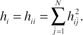 (6.22)
H=X(X′X)−1X′.
ˆy=Hy.
var(ˆy)=σ2H,
var(r)=σ2(1−H).
H=X[X′V(ˆΘ)−1X]−X′V(ˆΘ)−1.
 (6.26)
6.2.3. DFFITS, MDFFITS, COVTRACE, and COVRATIO Statistics
DFFITSi=ˆyi−ˆyi(−i)s(−i)√hi,
 (6.27)
DFFITSi=ti√hi1−hi.
 (6.28)
DFFITSi=ˆyi−ˆyi(−i)ese(ˆyi),
 (6.29)
ese(ˆyi)=√x′i[X′V(ˆΘ(−i))−X]−1xi,
 (6.30)
MDFFITS[β(−i)]=[ˆβ−ˆβ(−i)]′var[ˆβ(−i)]−[ˆβ−ˆβ(−i)]rank(X).
 (6.31)
 in Equation (6.31). is evaluated at ˆΘ(−i)
MDFFITS[Θ(−i)]=[ˆΘ−ˆΘ(−i)]′var[ˆΘ(−i)]−1[ˆΘ−ˆΘ(−i)].
 (6.32)
COVTRACE[β(−i)]=|trace{var(ˆβ)−var[ˆβ(−i)]}−rank(X)|,
 (6.33)
COVRATIO[β(−i)]=det{var[ˆβ(−i)]}det[var(ˆβ)],
 (6.34)
 indicates the determinant of the nonsingular part of the var[ˆβ(−i)] matrix. The COVRATIO statistic can be used to assess the precision of the fixed effects with the following criteria: if COVRATIO > 1, inclusion of subject i in the regression improves the precision of the parameter estimates; if COVRATIO < 1, the incorporation of the subject in the estimating process reduces the precision of the estimation, so that subject i may be deleted in the model fit.
COVTRACE[Θ(−i)]=|trace{var(ˆΘ)−var[ˆΘ(−i)]}−rank[var(ˆΘ)]|,
 (6.35)
COVRATIO[(Θ(−i))]=det{var[ˆΘ(−i)]}det[var(ˆΘ)].
 (6.36)
6.2.4. Likelihood Displacement Statistic Approximation
LDi=2l (ˆβ)−2l[ˆβ(−i)],
RLDi=2lR (ˆβ)−2lR[ˆβ(−i)],
 is the log-likelihood function and lR (ˆβ)
 is the log restricted likelihood function with respect to the estimated regression coefficients ˆβ
l(θ|w)=∑Ni=1wili(θ),
 (6.38a)
lR(θ|w)=∑Ni=1wilRi(θ),
 (6.38b)
LD(w)=2l (ˆθ)−2l[ˆθw],
RLD(w)=2lR(ˆθ)−2lR[ˆθw].
LDi(wi)≈˜U′iI−1(ˆθ)˜Ui,
6.2.5. LMAX Statistic for Identification of Influential Observations
B≈˜U′I−1(ˆθ)˜U,
 is positive definite, the N × N symmetric matrix B is positive semidefinite, with rank no more than M. The statistic ˜lmax
B˜lmax=¨λmax˜lmax and ˜lmax′˜lmax=1,
 When M > 1, an advantage of examining elements of the LMAX statistic is that each case has a single summary measurement of influence.
6.3. Empirical Illustrations on Influence Diagnostics
6.3.1. Influence Checks on Linear Mixed Model Concerning Effectiveness of Acupuncture Treatment on PCL Score

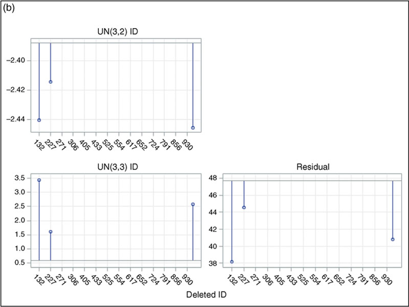
Table 6.1
Selected Influence Statistics for 10 Subjects: DHCC Acupuncture Treatment Study (N = 10)
| Subject’s ID | Influence Diagnostics for 10 Subjects | |||||
| Number of Observations | Number of Iterations | Cook’s D | MDFFITS on β | COVRATIO on β | LD Statistic | |
| 132 | 4 | 2 | 0.0533 | 0.0524 | 1.0080 | 0.5396 |
| 167 | 4 | 1 | 0.0114 | 0.0108 | 1.2674 | 0.1007 |
| 193 | 4 | 2 | 0.0242 | 0.0236 | 1.1246 | 0.2139 |
| 220 | 4 | 2 | 0.0134 | 0.0132 | 1.2960 | 0.1690 |
| 227 | 4 | 2 | 0.0195 | 0.0188 | 1.1914 | 0.1657 |
| 230 | 2 | 1 | 0.0006 | 0.0006 | 1.1728 | 0.0158 |
| 235 | 4 | 1 | 0.0263 | 0.0252 | 1.1858 | 0.2130 |
| 245 | 4 | 2 | 0.0358 | 0.0351 | 1.0913 | 0.3399 |
| 271 | 1 | 1 | 0.0000 | 0.0000 | 1.0785 | 0.0057 |
| 276 | 4 | 2 | 0.0324 | 0.0315 | 1.1090 | 0.3003 |

rather than var[ˆβ] in computation. The COVRATIO and the LD statistics are also fairly stable, thereby suggesting that none of these ten subjects has a strong impact on the fit of the linear mixed model on PCL_SUM. From the results of other influence diagnostics and for other subjects, no distinctively influential cases can be found.

Table 6.2
Maximum Likelihood Estimates and the Likelihood Displacement Statistic for Three Linear Mixed Models
| Explanatory Variable | Parameter Estimate | Standard Error | Degrees of Freedom | t-value | p-value |
| Linear Mixed Model With Full Data (-2 LL = 1411.3; p < 0.0001) | |||||
| Intercept | 55.444 | 2.509 | 53 | 22.10 | <0.0001 |
| Treatment | 2.698 | 3.516 | 53 | 0.77 | 0.4463 |
| Time 1 | −3.963 | 2.056 | 128 | −1.93 | 0.0561 |
| Time 2 | −2.977 | 2.168 | 128 | −1.37 | 0.1721 |
| Time 3 | −9.233 | 2.137 | 128 | −4.32 | <0.0001 |
| Treat × Time 1 | −14.494 | 3.007 | 128 | −4.82 | <0.0001 |
| Treat × Time 2 | −15.803 | 3.232 | 128 | −4.89 | <0.0001 |
| Treat × Time 3 | −8.666 | 3.177 | 128 | −2.73 | 0.0073 |
| Linear Mixed Model Deleting Subject 791 (-2 LL = 1371.3; p < 0.0001) | |||||
| Intercept | 56.231 | 2.550 | 52 | 22.05 | <0.0001 |
| Treatment | 1.912 | 3.542 | 52 | 0.54 | 0.5916 |
| Time 1 | −4.885 | 2.007 | 125 | −2.43 | 0.0164 |
| Time 2 | −4.359 | 2.122 | 125 | −2.05 | 0.0420 |
| Time 3 | −10.613 | 2.090 | 125 | −5.08 | <0.0001 |
| Treat × Time 1 | −13.537 | 2.908 | 125 | −4.65 | <0.0001 |
| Treat × Time 2 | −14.369 | 3.129 | 125 | −4.59 | <0.0001 |
| Treat × Time 3 | −7.229 | 3.075 | 125 | −2.35 | 0.0203 |
| LD statistic | 40.0 (df = 4; p < 0.01) | ||||
| Linear Mixed Model Deleting Subject 814 (-2 LL = 1368.6; p < 0.0001) | |||||
| Intercept | 54.923 | 2.535 | 52 | 21.67 | <0.0001 |
| Treatment | 3.220 | 3.520 | 52 | 0.91 | 0.3646 |
| Time 1 | −4.231 | 1.992 | 125 | −2.12 | 0.0356 |
| Time 2 | −3.338 | 2.106 | 125 | −1.59 | 0.1154 |
| Time 3 | −7.959 | 2.074 | 125 | −3.84 | 0.0002 |
| Treat × Time 1 | −14.189 | 2.886 | 125 | −4.92 | <0.0001 |
| Treat × Time 2 | −15.388 | 3.105 | 125 | −4.96 | <0.0001 |
| Treat × Time 3 | −9.880 | 3.052 | 125 | −3.24 | 0.0015 |
| LD statistic | 42.7 (df = 4; p < 0.01) | ||||
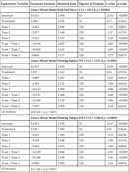
 , is statistically significant with four degrees of freedom and at α = 0.05 (LD = 40.0, p < 0.01), thereby indicating that this subject makes a very strong statistical impact on the overall fit of the first linear mixed model. Likewise, the third model is fitted after deleting subject 814, with the exact LD statistic also statistically significant at the same criterion (LD = 42.7, p < 0.01). Furthermore, in both the second and the third models, the parameter estimates, including the regression coefficients and the standard errors, vary notably after removing each of those two cases. Obviously, those two cases make a genuine impact in fitting the linear mixed model. Given the considerable changes in the estimated regression coefficients as well as the exceptionally strong statistical contributions, I would recommend that the two influential cases should be eliminated from the regression. The lack of statistical stability may also be linked to the small sample size for the data. For large samples, a strong relative influence of a few particular cases usually can be washed out by the effects of the vast majority of the normal observations in the estimating process. This argument will be further discussed in the next example where a large sample is analyzed.


6.3.2. Influence Diagnostics on Linear Mixed Model Concerning Marital Status and Disability Severity Among Older Americans

Table 6.3
Maximum Likelihood Estimates and the Likelihood Displacement Statistic for Three Linear Mixed Models on ADL Count: Older Americans
| Explanatory Variable | Parameter Estimate | Standard Error | Degrees of Freedom | t-value | p-value |
| Linear Mixed Model With Full Data (-2 LL = 20,016.3; p < 0.0001) | |||||
| Intercept | 0.673 | 0.044 | 1726 | 15.31 | <0.0001 |
| Married | 0.029 | 0.059 | 300 | 0.49 | 0.6223 |
| Time 1 | 0.257 | 0.036 | 4814 | 7.19 | <0.0001 |
| Time 2 | 0.513 | 0.052 | 4814 | 9.87 | <0.0001 |
| Time 3 | 0.579 | 0.058 | 4814 | 9.94 | <0.0001 |
| Time 4 | 0.768 | 0.061 | 4814 | 12.56 | <0.0001 |
| Time 5 | 0.932 | 0.060 | 4814 | 15.60 | <0.0001 |
| Treat × Time 1 | −0.159 | 0.053 | 4814 | −3.01 | 0.0026 |
| Treat × Time 2 | −0.252 | 0.078 | 4814 | −3.24 | 0.0012 |
| Treat × Time 3 | −0.233 | 0.090 | 4814 | −2.58 | 0.0099 |
| Treat × Time 4 | −0.060 | 0.098 | 4814 | −0.61 | 0.5441 |
| Treat × Time 5 | −0.309 | 0.101 | 4814 | −3.07 | 0.0021 |
| Linear Mixed Model Deleting Subject 200520020 (-2 LL = 20000.5; p < 0.0001) | |||||
| Intercept | 0.673 | 0.044 | 1725 | 15.29 | <0.0001 |
| Married | 0.028 | 0.059 | 300 | 0.48 | 0.6335 |
| Time 1 | 0.257 | 0.036 | 4809 | 7.18 | <0.0001 |
| Time 2 | 0.513 | 0.052 | 4809 | 9.87 | <0.0001 |
| Time 3 | 0.580 | 0.058 | 4809 | 9.94 | <0.0001 |
| Time 4 | 0.768 | 0.061 | 4809 | 12.56 | <0.0001 |
| Time 5 | 0.932 | 0.060 | 4809 | 15.60 | <0.0001 |
| Treat × Time 1 | −0.159 | 0.053 | 4809 | −3.01 | 0.0026 |
| Treat × Time 2 | −0.250 | 0.078 | 4809 | −3.21 | 0.0013 |
| Treat × Time 3 | −0.234 | 0.090 | 4809 | −2.59 | 0.0096 |
| Treat × Time 4 | −0.059 | 0.098 | 4809 | −0.60 | 0.5478 |
| Treat × Time 5 | −0.302 | 0.101 | 4809 | −3.00 | 0.0027 |
| LD statistic | 15.8 (df = 2; p < 0.01) | ||||
| Linear Mixed Model Deleting Subject 207669010 (-2 LL = 19985.0; p < 0.0001) | |||||
| Intercept | 0.675 | 0.044 | 1725 | 15.35 | <0.0001 |
| Married | 0.026 | 0.059 | 300 | 0.44 | 0.6599 |
| Time 1 | 0.255 | 0.036 | 4809 | 7.11 | <0.0001 |
| Time 2 | 0.513 | 0.052 | 4809 | 9.86 | <0.0001 |
| Time 3 | 0.578 | 0.058 | 4809 | 9.92 | <0.0001 |
| Time 4 | 0.770 | 0.061 | 4809 | 12.58 | <0.0001 |
| Time 5 | 0.923 | 0.060 | 4809 | 15.47 | <0.0001 |
| Treat × Time 1 | −0.156 | 0.053 | 4809 | −2.96 | 0.0031 |
| Treat × Time 2 | −0.252 | 0.078 | 4809 | −3.23 | 0.0012 |
| Treat × Time 3 | −0.231 | 0.090 | 4809 | −2.56 | 0.0105 |
| Treat × Time 4 | −0.061 | 0.098 | 4809 | −0.62 | 0.5324 |
| Treat × Time 5 | −0.300 | 0.100 | 4809 | −2.99 | 0.0028 |
| LD statistic | 31.3 (df = 6; p < 0.01) | ||||


 , is statistically significant with two degrees of freedom (this subject has two observations) and at α = 0.05 (LD = 15.8, p < 0.01), indicating that the most influential case makes a very strong statistical impact on the overall fit of the fixed effects. Likewise, the third mixed model is fitted after deleting the second most influential case (subject ID: 207669010), with the exact LD statistic also statistically significant with six degrees of freedom at the same criterion (LD = 31.3, p < 0.01). In both the second and the third models, however, the fixed estimates, including the regression coefficients and the standard errors, do not vary at all after removing each of those two cases. The fixed effects of the three control variables, not presented in Table 6.3, are also strikingly consistent after removing each of those two cases. The three sets of the estimated regression coefficients are almost identical. Obviously, deleting those two cases makes no genuine impact on the fixed-effects estimates, albeit strong statistical influences.

