
This chapter introduces techniques and considerations for mining the troves of data tucked away at LinkedIn, a popular and powerful social networking site focused on professional and business relationships. You’re highly encouraged to build up a professional LinkedIn network as you follow along with this chapter, but even if you don’t have a LinkedIn profile, you can still apply many of the techniques we’ll explore to other domains that provide a means of exporting information similar to that you’d find in an address book. Although LinkedIn may initially seem like any other social network, the data its API provides is inherently of a different nature. Generally speaking, people who care enough to join LinkedIn are interested in the business opportunities that it provides and want their profiles to look as stellar as possible—which means ensuring that they provide ample details of a fairly personal nature conveying important business relationships, job details, etc.
Given the somewhat sensitive nature of the data, the API is somewhat different than many of the others we’ve looked at in this book. For example, while you can generally access all of the interesting details about your contacts’ educational histories, previous work positions, etc., you cannot determine whether two arbitrary people are “connected,” and the absence of such an API method is not accidental—this decision was made because the management team at LinkedIn strongly believes that your professional networking data is inherently private and far too valuable to open up to the same possibilities of exploitation as, say, knowledge about your Twitter or Facebook friends.[37]
Given that LinkedIn limits your access to information about your direct connections and does not lend itself to being mined as a graph, it requires that you ask different types of questions about the data that’s available to you. The remainder of this chapter introduces fundamental clustering techniques that can help you answer the following kinds of queries:
Which of your connections are the most similar based upon a criterion like job title?
Which of your connections have worked in companies you want to work for?
Where do most of your connections reside geographically?
Given the richness of LinkedIn data, being able to answer queries about your professional networks presents some powerful opportunities. However, in implementing solutions to answer these types of questions, there are at least two common themes we’ll encounter over and over again:
It’s often necessary to measure similarity between two values (usually string values), whether they’re job titles, company names, professional interests, or any other field you can enter in as free text. Chapter 7 officially introduces some additional approaches and considerations for measuring similarity that you might want to also review.
In order to cluster all of the items in a set using a similarity metric, it would be ideal to compare every member to every other member. Thus, for a set of n members, you would perform somewhere on the order of n2 similarity computations in your algorithm for the worst-case scenario. Computer scientists call this predicament an n-squared problem and generally use the nomenclature O(n2) to describe it;[38] conversationally, you’d say it’s a “Big-O of n-squared” problem. However, O(n2) problems become intractable for very large values of n. Most of the time, the use of the term “intractable” means you’d have to wait years (or even hundreds of years) for a solution to be computed—or, at any rate, “too long” for the solution to be useful.
These two issues inevitably come up in any discussion involving what is known as the approximate matching problem,[39] which is a very well-studied (but still difficult and messy) problem that’s ubiquitous in nearly any industry.
Techniques for approximate matching are a fundamental part of any legitimate data miner’s tool belt, because in nearly any sector of any industry—ranging from defense intelligence to fraud detection at a bank to local landscaping companies—there can be a truly immense amount of semi-standardized relational data that needs to be analyzed (whether the people in charge realize it or not). What generally happens is that a company establishes a database for collecting some kind of information, but not every field is enumerated into some predefined universe of valid answers. Whether it’s because the application’s user interface logic wasn’t designed properly, because some fields just don’t lend themselves to having static predetermined values, or because it was critical to the user experience that users be allowed to enter whatever they’d like into a text box, the result is always the same: you eventually end up with a lot of semistandardized data, or “dirty records.” While there might be a total of N distinct string values for a particular field, some number of these string values will actually relate the same concept. Duplicates can occur for various reasons: erroneous misspellings, abbreviations or shorthand, differences in the case of words, etc.
Although it may not be obvious, this is exactly the situation we’re faced with in mining LinkedIn data: LinkedIn members are able to enter in their professional information as free text, which results in a certain amount of unavoidable variation. For example, if you wanted to examine your professional network and try to determine where most of your connections work, you’d need to consider common variations in company names. Even the simplest of company names have a few common variations you’ll almost certainly encounter. For example, it should be obvious to most people that “Google” is an abbreviated form of “Google, Inc.”, but even these kinds of simple variations in naming conventions must be explicitly accounted for during standardization efforts. In standardizing company names, a good starting point is to first consider suffixes such as “, Inc.”, “, LLC”, etc. Assuming you had a comma-separated values (CSV) file of contacts that you’d exported from LinkedIn, you might start out by doing some basic normalization and then printing out selected entities from a histogram, as illustrated in Example 6-1.
The two primary ways you can access your LinkedIn data are by either
exporting it as address book data, which maintains very basic information
such as name, job title, company, and contact information, or using the
LinkedIn API to programmatically exploit the full details of your
contacts. While using the API provides access to everything that would be
visible to you as an authenticated user browsing profiles at http://linkedin.com, we can get all of the job title
details we need for this first exercise by exporting address book
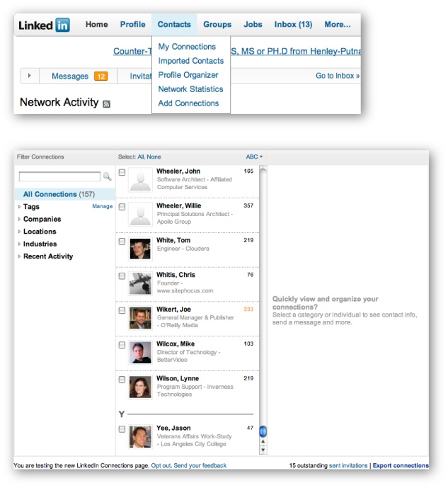
information. (We’ll use LinkedIn APIs later in this chapter, in Fetching Extended Profile Information.) In case it’s not obvious how to export your
connections, Figure 6-1 provides some
visual cues that show you how to make it happen. We’ll be using Python’s
csv module to parse the exported data;
to ensure compatibility with the upcoming code listing, choose the
“Outlook CSV” option.
Example 6-1. Simple normalization of company suffixes from address book data (linkedin__analyze_companies.py)
# -*- coding: utf-8 -*-

import sys
import nltk
import csv
from prettytable import PrettyTable

CSV_FILE = sys.argv[1]

# Handle any known abbreviations,
# strip off common suffixes, etc.

transforms = [(', Inc.', ''), (', Inc', ''), (', LLC', ''), (', LLP', '')]

csvReader = csv.DictReader(open(CSV_FILE), delimiter=',', quotechar='"')
contacts = [row for row in csvReader]
companies = [c['Company'].strip() for c in contacts if c['Company'].strip() != '']

for i in range(len(companies)):
    for transform in transforms:
        companies[i] = companies[i].replace(*transform)

pt = PrettyTable(fields=['Company', 'Freq'])
pt.set_field_align('Company', 'l')
fdist = nltk.FreqDist(companies)
[pt.add_row([company, freq]) for (company, freq) in fdist.items() if freq > 1]
pt.printt()
However, you’d need to get a little more sophisticated to handle more complex situations, such as the various manifestations of company names like O’Reilly Media that you might encounter. For example, you might see this company’s name represented as O’Reilly & Associates, O’Reilly Media, O’Reilly, Inc.,[40] or just O’Reilly. The very same problem presents itself in considering job titles, except that it can get a lot messier because job titles are so much more variable. Table 6-1 lists a few job titles you’re likely to encounter in a software company that include a certain amount of natural variation. How many distinct roles do you see for the 10 distinct titles that are listed?
Table 6-1. Example job titles for the technology industry
| Job Title |
|---|
| Chief Executive Officer |
| President/CEO |
| President & CEO |
| CEO |
| Developer |
| Software Developer |
| Software Engineer |
| Chief Technical Officer |
| President |
| Senior Software Engineer |
While it’s certainly possible to define a list of aliases or abbreviations that equate titles like CEO and Chief Executive Officer, it may not be very practical to manually define lists that equate titles such as Software Engineer and Developer for the general case in all possible domains. However, for even the messiest of fields in a worst-case scenario, it shouldn’t be too difficult to implement a solution that condenses the data to the point that it’s manageable for an expert to review it, and then feed it back into a program that can apply it in much the same way that the expert would have done. More times than not, this is actually the approach that organizations prefer since it allows humans to briefly insert themselves into the loop to perform quality control.
[37] LinkedIn’s position was relayed in a discussion between the author and D.J. Patil, Chief Scientist, Chief Security Officer, and Senior Director—Project Analytics at LinkedIn.
[38] Technically speaking, it is sometimes more precise to describe the time complexity of a problem as Θ(n2), because O(n2) represents a worst case, whereas Θ(n2) represents a tighter bound for the expected performance. In other words, Θ(n2) says that it’s not just an n2 problem in the worst case, it’s an n2 problem in the best case, too. However, our objective in this chapter isn’t to analyze the runtime complexity of algorithms (a difficult subject in and of itself), and we’ll stick with the more common O(n2) notation and describing the worst case.
[39] Also commonly called fuzzy matching, clustering, and/or deduplication, among many other things. Trying to perform approximate matching on multiple fields (records) is commonly referred to as the “record linkage” problem.
[40] If you think this is starting to sound complicated, just consider the work taken on by Dun & Bradstreet (the “Who’s Who” of company information), the company that is blessed with the challenge of maintaining a worldwide directory that identifies companies spanning multiple languages from all over the globe.